Article

Using Remote Sensing Products for Environmental Analysis in South America

by
Francielle da Silva Cardozo
*,
Yosio Edemir Shimabukuro
,
Gabriel Pereira
and
Fabrício Brito Silva
Remote Sensing Division (DSR), National Institute for Space Research, Av. dos Astronautas, 1758 Jd. Granja, São José dos Campos, SP 12227-010, Brazil
*
Author to whom correspondence should be addressed.
Remote Sens. 2011, 3(10), 2110-2127; https://doi.org/10.3390/rs3102110
Submission received: 21 July 2011 / Revised: 2 September 2011 / Accepted: 12 September 2011 / Published: 26 September 2011
(This article belongs to the Special Issue 100 Years ISPRS - Advancing Remote Sensing Science)

Abstract

:
Land cover plays a major role in many biogeochemical models that represent processes and connections with terrestrial systems; hence, it is a key component for public decisions in ecosystems management. The advance of remote sensing technology, combined with the emergence of new operational products, offers alternatives to improve the accuracy of environmental monitoring and analysis. This work uses the GLOBCOVER, the Vegetation Continuous Field (VCF), MODIS Fire Radiative Power (FRP) and the Tropical Rainfall Measuring Mission (TRMM) remotely sensed databases to analyze the biomass burning distribution, the land use and land cover characteristics and the percent of tree cover in South America during the years 2000 to 2005. Initially, GLOBCOVER was assessed based on VCF product, and subsequently used for quantitative analysis of the spatial distribution of the South America fires with the fire radiative power (FRP). The results show that GLOBCOVER has a tendency to overestimate forest classes and to underestimate urban and mangroves areas. The fire quantification based on GLOBCOVER product shows that the highest incidence of fires can be observed in the arc of deforestation, located in the Amazon forest border, with vegetation cover composed mainly of broadleaved evergreen or semi-deciduous forest. A time series analysis of FRP database indicates that biomass burning occurs mainly in areas of broadleaved evergreen or semi-deciduous forest and in Brazilian Cerrado associated with grassland management, agricultural land clearing and with the deforestation of Amazon tropical rainforest. Also, variations in FRP intensity and spread can be attributed to rainfall anomalies, such as in 2004, when South America had a positive anomaly rainfall.

Graphical Abstract

1. Introduction

Land cover plays a major role in many environmental models that represent processes and connections between surface and atmospheric processes, which modify the energy balance [1,2,3,4,5,6,7], atmospheric chemistry [8,9,10,11], evapotranspiration and precipitation [12,13]. Hence, land cover is a key component for public decisions on ecosystems management and in the assessment of the impacts of anthropogenic actions on the equilibrium of ecosystems.
Over time, biomass burning consumes vast areas of grassland and forests around the globe, releasing large and unknown quantities of aerosols and trace gases into the atmosphere [8]. In South America, land use and land cover (LULC) maps show temporal and spatial variability in anthropogenic biomass burning, which are directly associated with agricultural land clearing, grassland management and with the deforestation of Amazon tropical rainforest. The highest incidences of fires can be observed in the arc of deforestation, located in the Amazon forest border [14,15].
Fire characteristics and intensity can be defined in terms of their energy released in the combustion process. The fraction of chemical energy emitted from burning biomass as radiation can be defined as Fire Radiative Power (FRP). FRP can be estimated via an airborne infrared radiometer [16] and also through infrared bands derived from environmental satellites such as the Moderate Resolution Imaging Spectroradiometer (MODIS). In theory, radiative intensity released by fires is linearly correlated with the burned biomass and might be independent of vegetation type [17,18]. Also, satellite measurements of FRP released rate can be associated with aerosol optical depth (AOD) to provide regional smoke emission coefficients [19]. Studies analyzing the biomass burning patterns using FRP for global characterization were be performed by Ichoku et al. [20], for Africa by Roberts et al. [21], Roberts and Wooster [22] and for Asia by Vadrevu et al. [23].
The improvement of remote sensing techniques, combined with the advent of new products and operational satellites, allows obtaining information of physicochemical and biological properties of large areas of surface. Currently, the number of environmental satellite sensors acquiring images of the earth’s surface has been increasing significantly. In the literature, several remote sensing-based land cover maps were developed from a large number of sources [24,25,26,27,28,29,30], however, each product has a specificity and presents advantages and disadvantages [31].
The GLOBCOVER project is an initiative of European Space Agency (ESA) in cooperation with international institutions; it is useful in monitoring the dynamics of land cover and forests [16]. The Earth Observing System (EOS) initiative of National Aeronautics and Space Administration (NASA) is another program that provides important data for environmental monitoring of land, ocean and atmospheric ecosystems. Many products provided by the MODIS sensor aboard AQUA and TERRA platforms such as the Vegetation Continuous Field (VCF), Normalized Difference Vegetation Index (NDVI), Enhanced Vegetation index (EVI), Leaf Area Index (LAI) and Gross Primary Productivity, allow phenological studies in annual time series [32].
Despite the efforts of each program in implementing environmental, hardware, software and data distribution, these aforementioned products have their respective limitations, inherent to each type of processing, leading to confusion in the identification and delineation of different land use and land cover [33]. Most of land cover products are generated from coarse resolution satellite imagery and addressed to characterizing the global land use and land cover characteristics. Several studies could be found in the literature that perform analysis of distinct products comparing the classified data with available land use and land cover products or ground truth [31,34,35,36,37]. These authors found errors that vary substantially between land use and land cover datasets and are related to mixed tree cover types, similar spectral response and spatial distribution. Also, there are some classes that show higher accuracy values composed of homogenous areas, such as broadleaf forest and snow areas. Moreover, urban areas and croplands show high commission errors.
Thus, the main objective of this work is to perform an environmental analysis from remote sensing products derived for all of South America, including GLOBCOVER land use and land cover, MODIS VCF tree cover, Tropical Rainfall Measuring Mission (TRMM) rainfall rate and FRP data derived from MODIS and Geostationary Operational Environmental Satellite (GOES). Initially, the GLOBCOVER was evaluated with VCF product and, subsequently, we performed an analysis of the spatial patterns of FRP distribution to each GLOBCOVER and VCF class relating this phenomenon with rainfall rate estimated by the TRMM as well as with amount of forest present in South America.

2. Data and Methodology
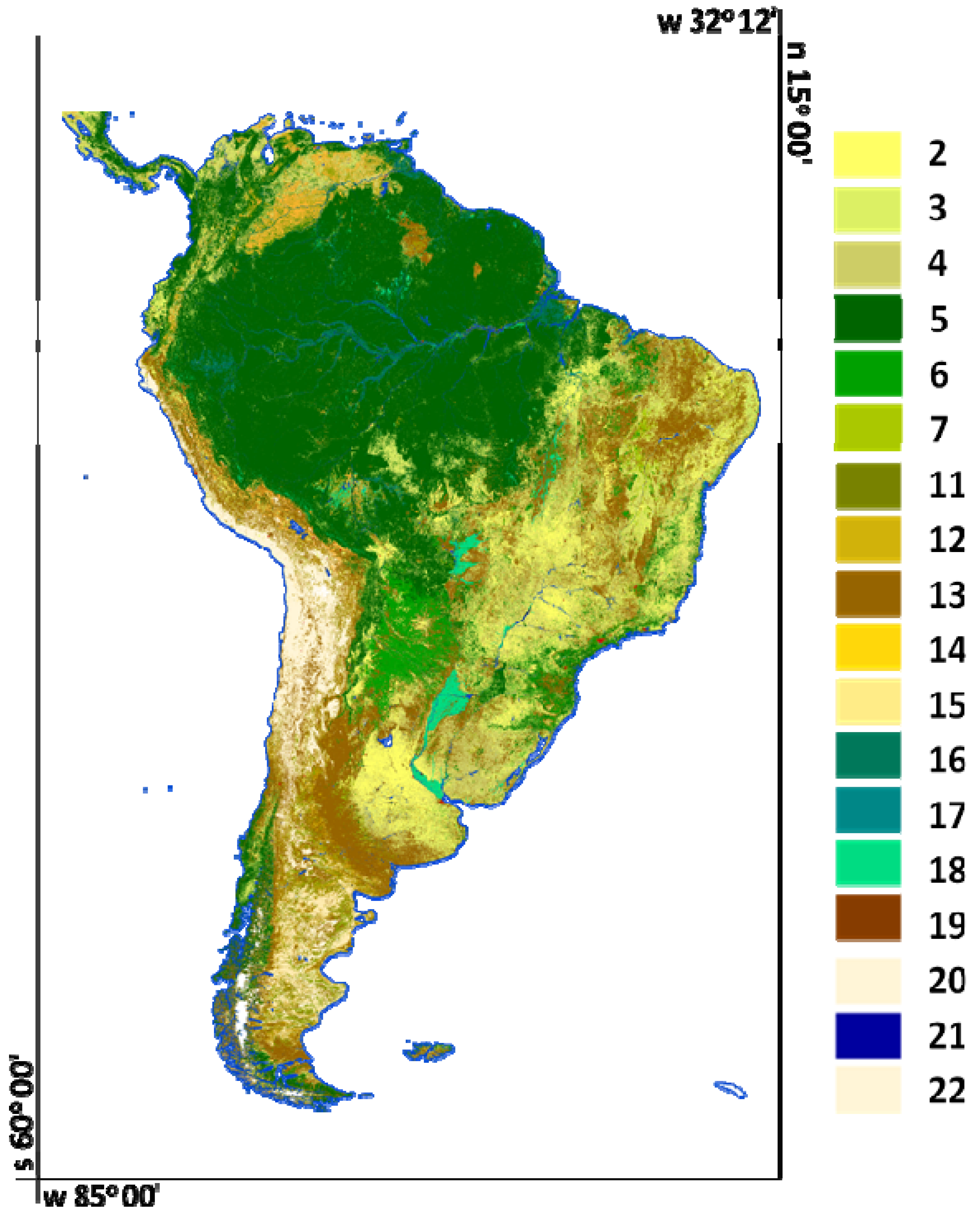
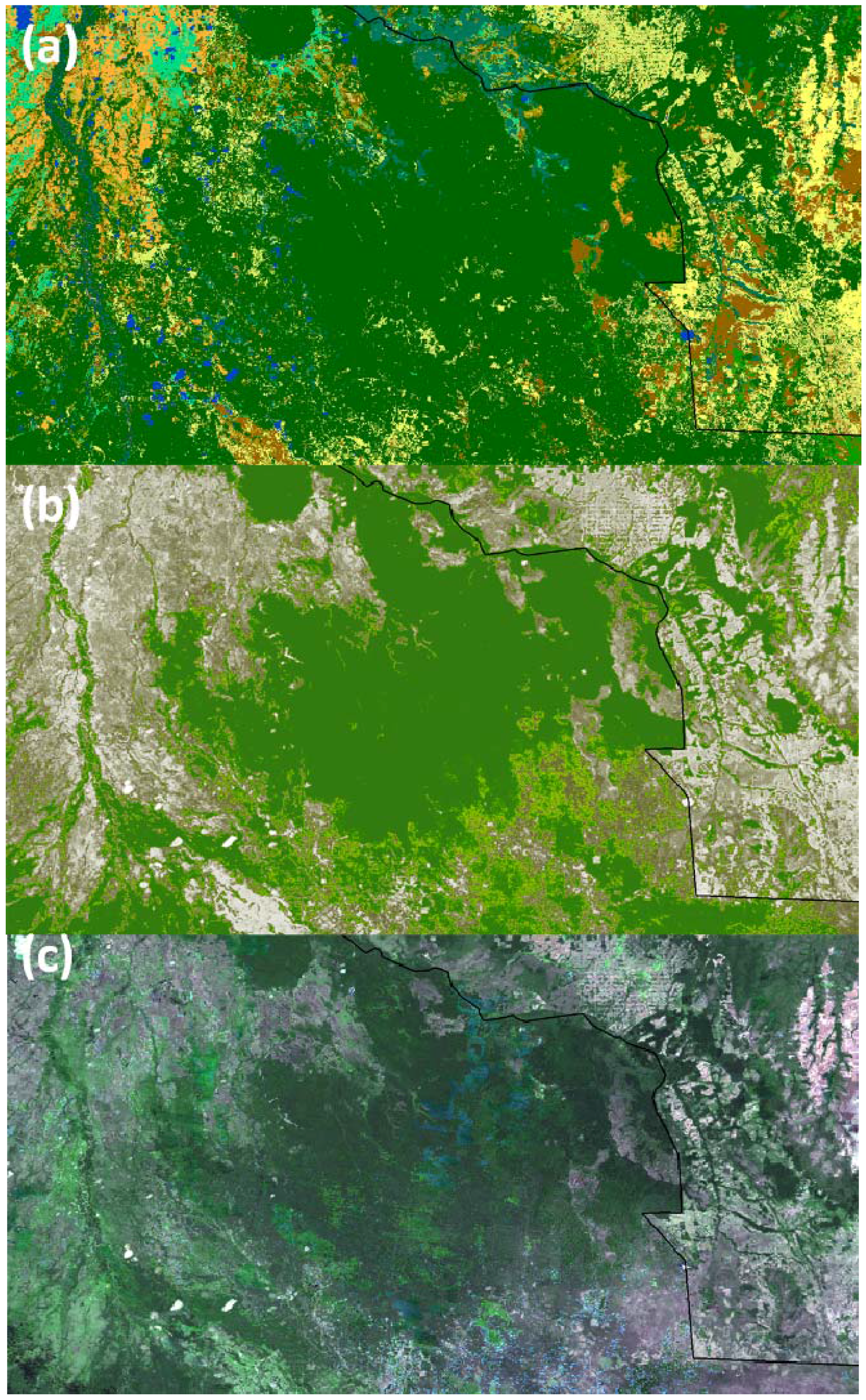
2.1. GLOBCOVER

Figure 1 shows the South America GLOBCOVER product. South America has a distinct and important biodiversity in the world, spatially distributed in its many natural ecosystems. However, this complex system is constantly exposed to anthropogenic activities such as deforestation, agriculture expansion and burning [15]. The objective of the ESA-GLOBCOVER project is the production of a land cover map of the world using an automated processing chain on 300 meter MERIS time series. The GLOBCOVER Land Cover map for the period of December 2004 to June 2006 is derived by an automatic and regionally-tuned classification of a MERIS full resolution (FR) time series. Its 22 land cover classes are defined with the UN Land Cover Classification System (LCCS) [30,38]. Assessment of GLOBCOVER product shows an overall accuracy of 70%, however, the land cover map varies according to regions and to land surface patterns [38].
One of the possible applications of GLOBCOVER products is the input for climate change models at regional and global scales. Also, GLOBCOVER could be used as input to a number of numeric models (energy cycles, land atmosphere interactions, hydrological), to analyze the differences in forest fragmentation [39]. Also, this product has applicability to studies of land-cover and land-use dynamics, improving the analysis of social dynamics of land management.
Figure 1. GLOBCOVER regional land use and land cover map for South America by automatic processing of temporal data obtained from the MERIS sensor with spatial resolution of 300 meters for the period from December 2004 to June 2006.
Remotesensing 03 02110 g001
In South America (Figure 1) the following classes are found [19]:
Table 1. GLOBCOVER land use and land cover classes.
NumberLand use and land cover class
2Rainfed croplands
3Mosaic cropland (50–70%)/vegetation (grassland/shrubland/forest) (20–50%);
4Mosaic vegetation (grassland/shrubland/forest) (50–70%)/cropland (20–50%)
5Closed to open (>15%) broadleaved evergreen or semi-deciduous forest (>5 m)
6Closed (>40%) broadleaved deciduous forest (>5 m)
7Open (15–40%) broadleaved deciduous forest/woodland (>5 m)
11Mosaic forest or shrubland (50–70%)/grassland (20–50%)
12Mosaic grassland (50–70%)/forest or shrubland (20–50%)
13Closed to open (>15%) (broadleaved or needleleaved, evergreen or deciduous) shrubland (<5 m)
14Closed to open (>15%) herbaceous vegetation (grassland, savannas or lichens/mosses)
15Sparse (<15%) vegetation
16Closed to open (>15%) broadleaved forest regularly flooded (semi-permanently or temporarily)—Fresh or brackish water
17Closed (>40%) broadleaved forest or shrubland permanently flooded—Saline or brackish water
18Closed to open (>15%) grassland or woody vegetation on regularly flooded or waterlogged soil—Fresh, brackish or saline water
19Artificial surfaces and associated areas (Urban areas >50%)
20Bare areas
21Water bodies
22Permanent snow and ice
Figure 2. 2005 South America Vegetation Continuous Fields product indicating the percent tree cover map derived from 500 m MODIS. In this product, higher values (greater than 80%, in green) suggests a ground surface covered by dense vegetation composed mainly of broadleaved forests and mixed forests, consequently, low values (less than 40%, in brown/grey) represents bare soil, herbaceous, grasslands and shrubland cover.
Remotesensing 03 02110 g002

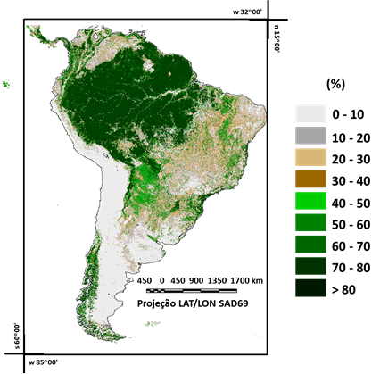
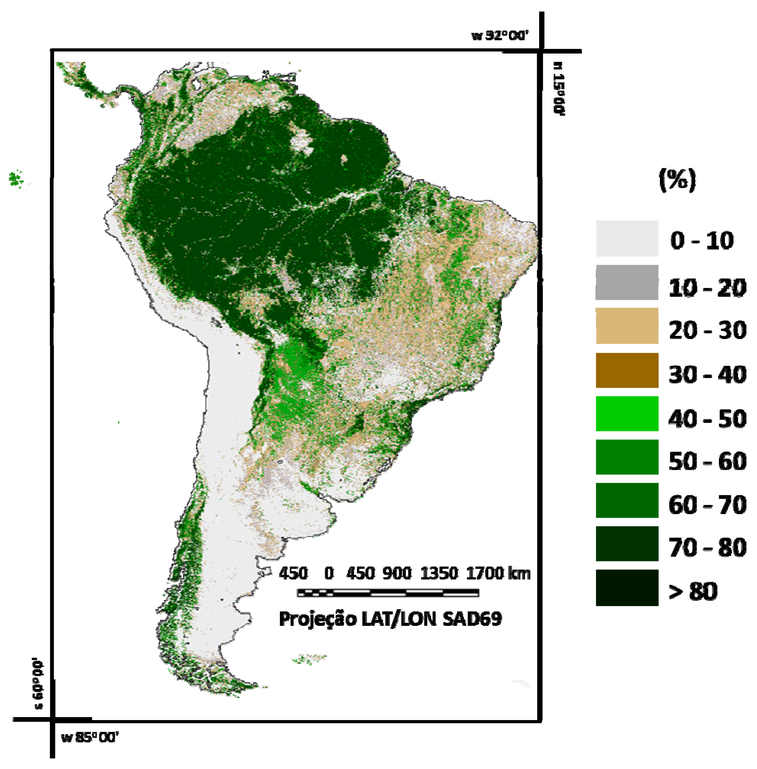
2.2. Vegetation Continuous Fields (VCF)

The VCF is a global percent tree cover map based on 500 m MODIS data, and represents the finest scale global forest information (Figure 2) [32,40]. The VCF data are used for biogeochemical cycles studies, ecosystem management and environmental analysis [41,42]. VCF product has been validated over continental and regional scales by several works [32,40,42], and the results indicate an overall accuracy varying from 0.70 to 0.90 [43]. The VCF algorithm is an automated procedure which employs a regression tree algorithm, in which the percent canopy refers to the amount of skylight obstructed by tree canopies equal or greater than 5 m in height [32].

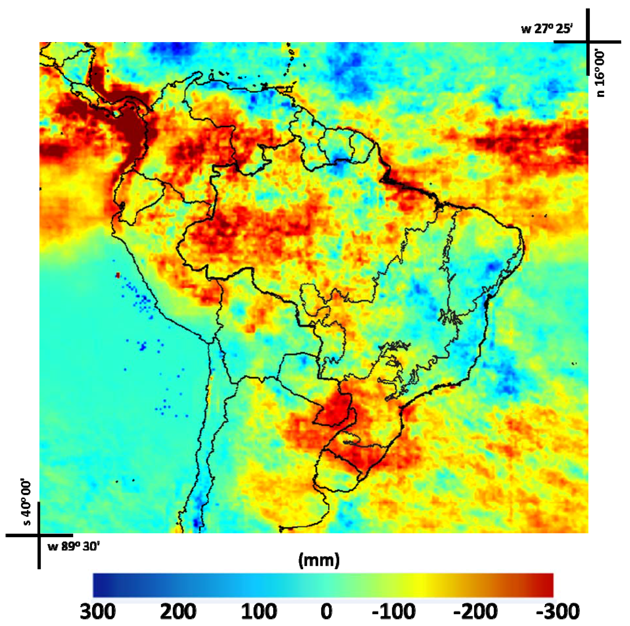
2.3. Tropical Rainfall Measuring Mission (TRMM)

The TRMM satellite data are used in this study to characterize the seasonal pattern of precipitation. The TRMM satellite is a partnership between NASA and the Japan Aerospace Exploration Agency (JAXA). Since 1997, these agencies have collected precipitation data encompassing more than two thirds of global precipitation. These data are generated by an algorithm that estimates the combined global precipitation estimations from multiple orbital sensors [44]. The data used in this work are related to the 3B42 product with daily temporal resolution; geographic covering: latitude from 50°S to 50°N and longitude from 180°W to 180°E; and horizontal resolution of 0.25° × 0.25°.

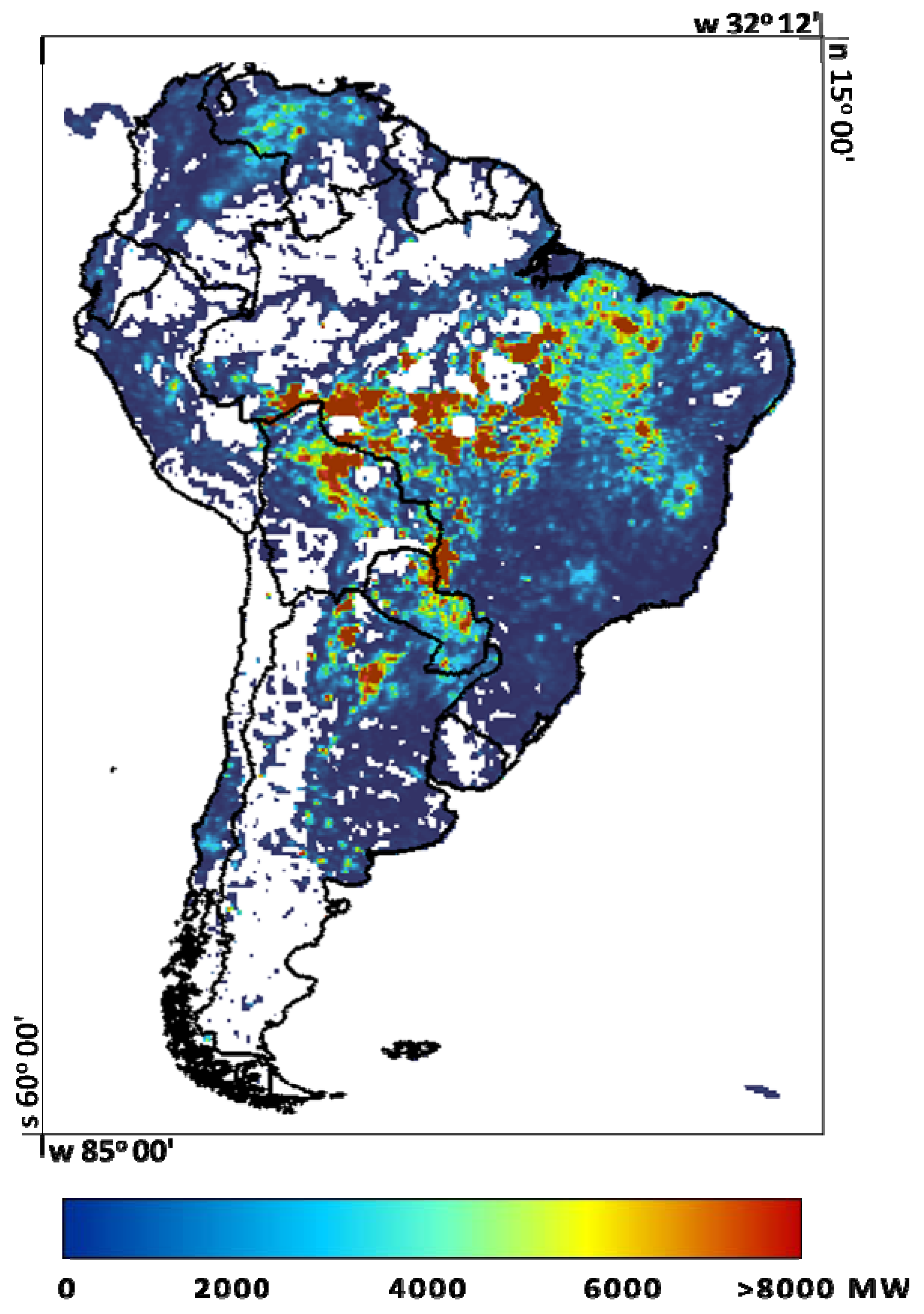
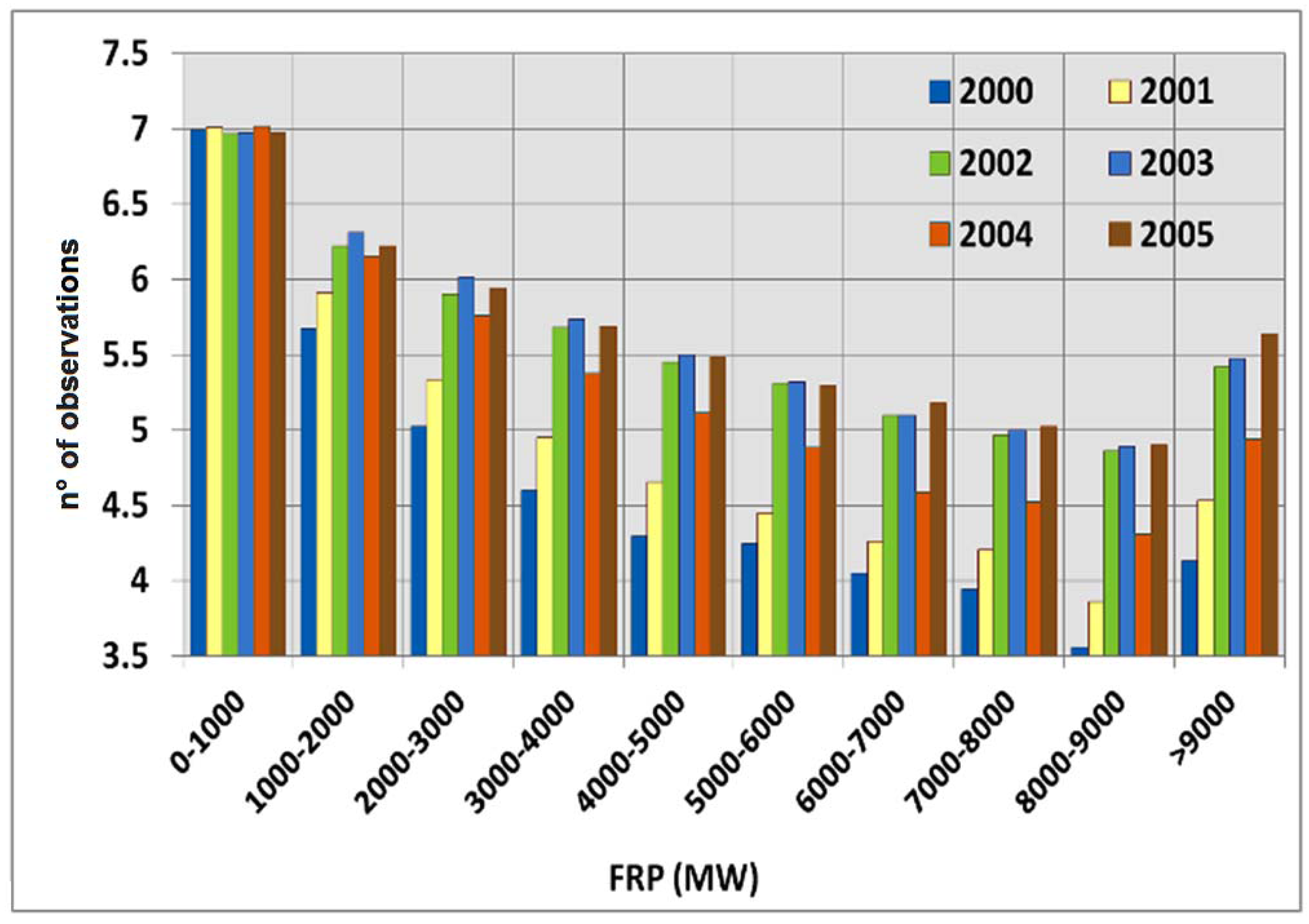
2.4. Fire Radiative Power (FRP)

The fraction of chemical energy emitted in biomass burning as electromagnetic radiation can be defined as Fire Radiative Power (FRP). Temporal integration of FRP gives the Fire Radiative Energy (FRE). Moreover, the FRE can be indicative of the amount of particulate matter and trace gases emitted into the atmosphere over a region [45]. Initial studies with FRP were performed with MODIS Airborne Simulator (MAS) in the Smoke, Cloud and Radiation-California/Brazil (SCAR-C and SCAR-B) experiments. In this work we used MODIS fire products, also called MOD14 (Terra) and MYD14 (Aqua); and Wildfire Automated Biomass Burning Algorithm (WFABBA) aboard GOES. The first product utilizes a contextual algorithm applied to brightness temperatures in 4 µm and 11 µm mid-infrared radiation channels; and the second is estimated by mid infrared radiance values. For each fire detection, FRP is calculated by the method proposed by [1,17,46,47], respectively:
FRPMODIS = 4.3 × 10¹⁹. (T8f 4µmT8b 4µm). Asample
F R P G O E S = A s a m p l e a σ ε B ( λ , T ) d λ L b
where Tf 4µm and Tb 4µm are, respectively, the MODIS brightness temperatures of the fire and the non-fire background in Kelvin (K), Asample is the real area of the pixel, a is a constant based on spectral response of GOES sensor (W.m−2.sr−1.µm−1.K−4), Lb is the background radiance (W.m−2.sr−1.µm−1), B is the Planck’s Law (W.m−2.sr−1.µm−1), σ is the Stefan-Boltzmann constant (5.67 × 10⁻⁸ J.s−1.m−2.K−4), ε is the emissivity and FRP is the Fire Radiative Power in Megawatts (MW) as shown for the 2005 MODIS fire data (Figure 3).
Figure 3. Fire radiative energy released in 2005 South America burning season derived from MODIS thermal anomalies/fire products (MOD14 and MYD14 level-2 swath) estimated four times a day from the Terra (10:30 and 22:30) and AQUA (13:30 and 01:30) platforms. In this product, higher values (in yellow/red) indicate areas with high incidence of large fires.
Remotesensing 03 02110 g003

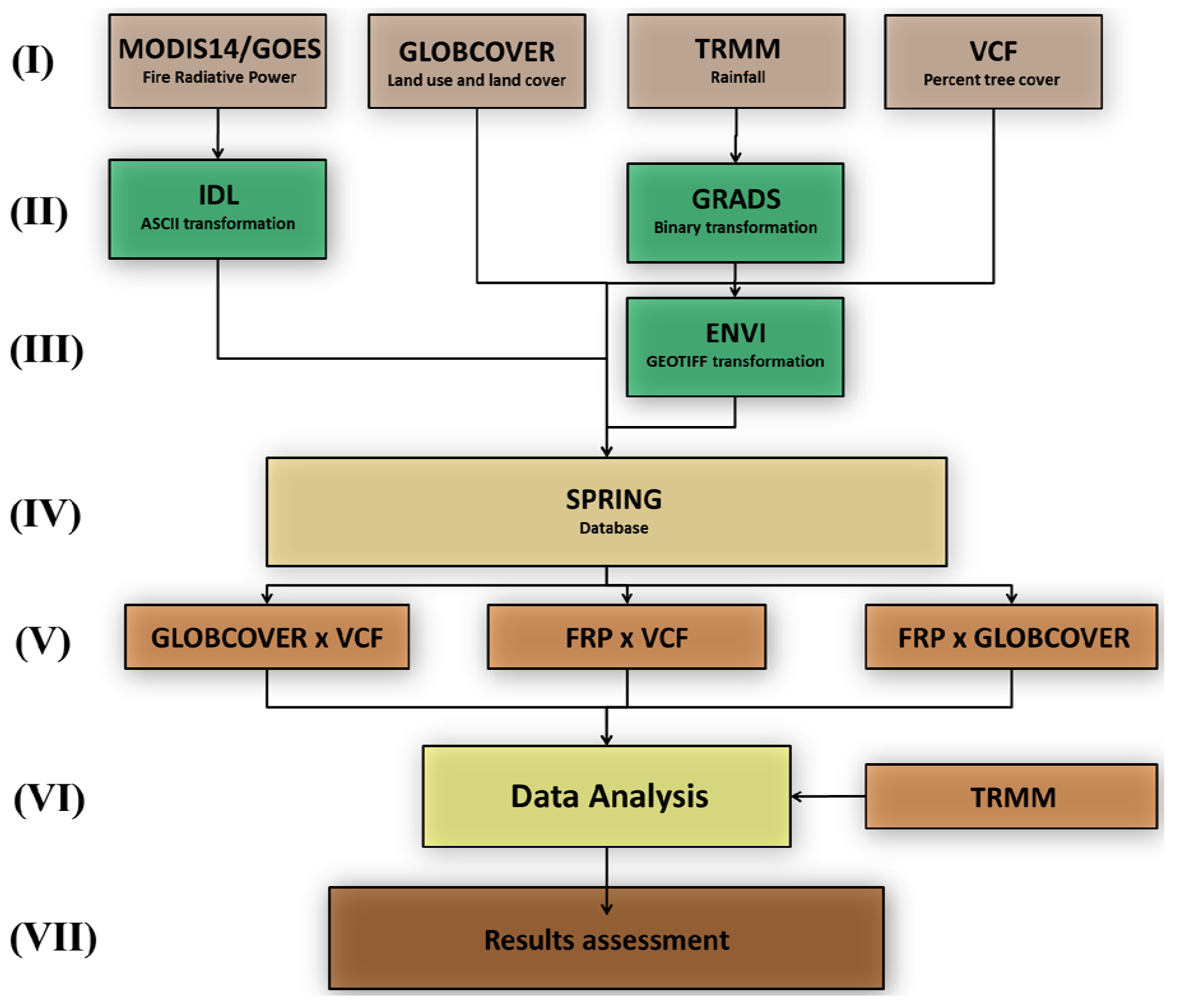
2.5. Data Processing

Geographic digital information is essential to support the knowledge and management of the environment, symbolizing a partial representation of the real world on computer. These representations of reality must be linked to geographical space, through its geographical coordinates. Consequently, geographic information systems (GIS) facilitate the analysis, management and manipulation of environmental information. The data of the above products were inserted into Georeferenced Information Processing System (SPRING), a state-of-the-art GIS program for managing and processing raster and vector data representations with an object-oriented data model developed by the National Institute for Space Research (INPE). Some procedures such as data format transformations and compatibility, attributes extraction and geographical analysis were made in the Spatial Algebraic Language for GIS (LEGAL), a spatial analysis tool that uses map algebra [48]. This language works from a command line and was proposed by Câmara [48] to assess spatial operations and statistical analysis.
Figure 4 shows the flowchart of the adopted methodology composed mainly of seven steps. The first step (I) was comprised of data acquisition of MODIS thermal anomalies/fire products (MOD14 and MYD14 level-2 swath data, available on https://wist.echo.nasa.gov), GLOBCOVER land use and cover product for South America (available on http://ionia1.esrin.esa.int), daily TRMM and other rainfall estimate product (3B42 V6 derived, available on http://disc2.nascom.nasa.gov/Giovanni/tovas) and VCF global percent tree cover map (available on http://www.landcover.org/data/vcf). The second and third stages (II and III), are composed of data transformation in which MODIS fire products, in hierarchical data format (HDF), were converted to ASCII format using Interactive Data Language (IDL), resulting in latitude, longitude and FRP columns. Also, the daily TRMM data were converted to monthly rainfall (mm.month−1) and transformed in binary format, and then were imported in Environment for Visualizing Images (ENVI) and converted to GEOTIFF format.
Figure 4. Flowchart of the methodology divided into seven steps: (I) Data acquisition; (II) and (III) Data transformation and processing; (IV) Creation of geographic information system using SPRING software; (V) Cross tabulation of GLOBCOVER, Vegetation Continuous Field (VCF) and Fire Radiative Power (FRP) products; (VI) and (VII) Results analysis and assessment.
Remotesensing 03 02110 g004
Normalized and converted satellite derived datasets were imported to SPRING database (step IV). In step (V), derived data (GLOBCOVER, VCF, FRP) were compared in pairs by cross tabulation and visual assessment. Cross tabulation is defined as a spatial operator that performs a measurement of intersections of thematic classes, resulting in a two-dimensional table with similarities and errors. After processing, thematic VCF and FRP were clustered in intervals of 10 (%) and 1,000 (MW), respectively, and results were analyzed and discussed (steps VI and VII).
The selection of the thresholds of VCF product to assessment of GLOBCOVER product were made according to land cover types selected by Hansen et al. [32] to train the linear mixture model (used to generate the percentage of tree cover map). In this work, the authors utilized a proportion of pixel area occupied by arboreous vegetation of approximately 80% (70–80% VCF class) to describe broadleaf evergreen forest, deciduous broadleaf forest and mixed forest. Moreover, land cover composed of woodlands and wooded grasslands/shrubland exhibit a pixel area occupied by herbaceous vegetation of approximately 50% and 75% (50% and 25% of arboreous vegetation), representing VCF values less than 40–50%. Thus, the thresholds proposed in [32] were applied in cross tabulation between GLOBCOVER and VCF products to analyze the assessment of both products.

3. Results and Discussion

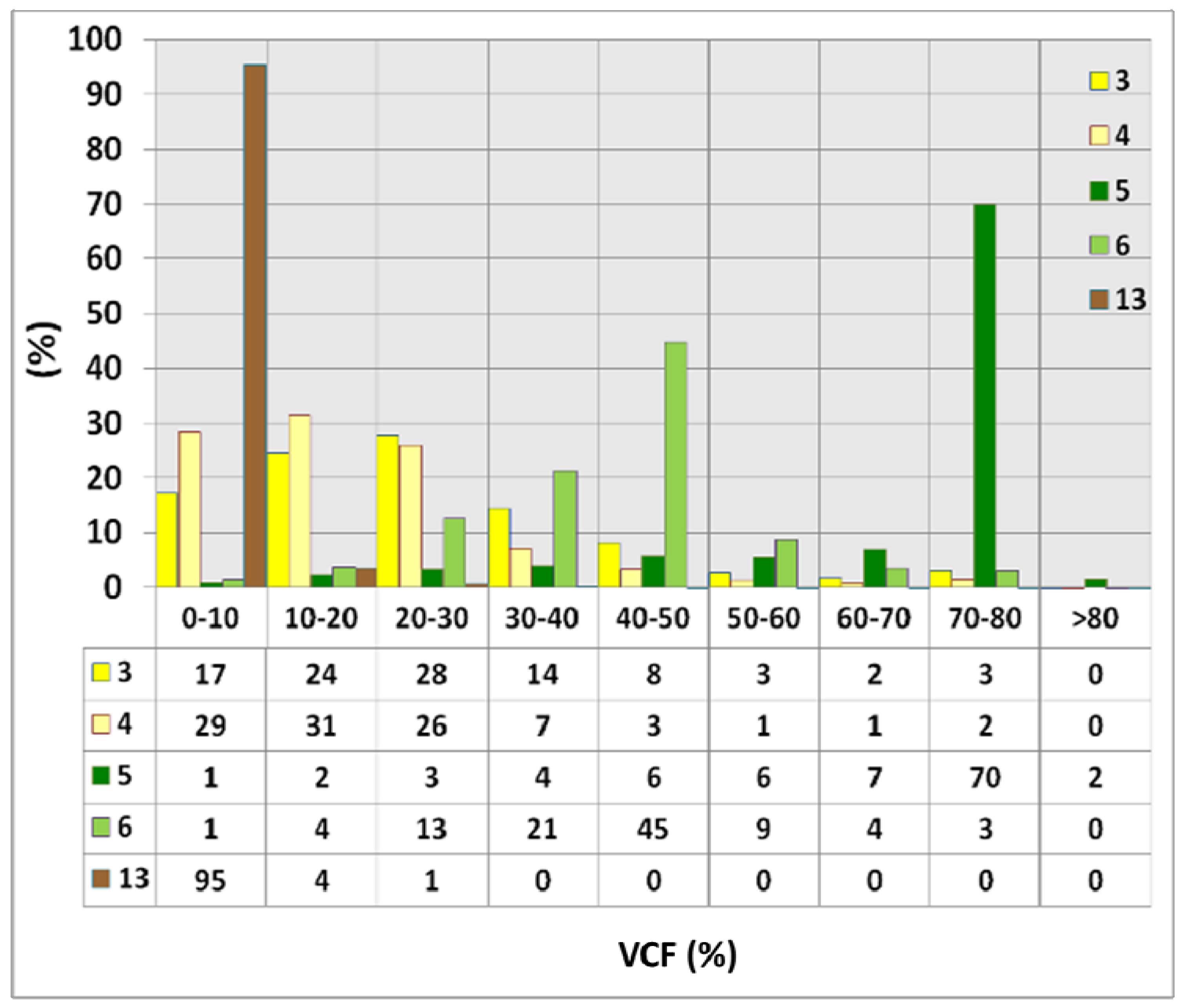
3.1. GLOBCOVER Assessment with VCF

The GLOBCOVER product characterizes South America LULC in 19 classes, which approximately 40% represents broadleaved evergreen or semi-deciduous forests such as Amazon forest and Atlantic Forest (tropical and subtropical moist forest), 17% is a merger of vegetation (grassland/shrubland/forest) and cropland (GLOBCOVER classes 2 and 3), 16% represents closed to open broadleaved or needle-leaved evergreen or deciduous shrubland and 6% is rainfed croplands. Also, there are minority class areas such as bare areas (3%), Sparse Vegetation (3%) and Grassland/Shrubland Forest (9%).
Operational landscape characterization methodologies could introduce systematic errors due to surface elements with spectral signature similarities [49,50,51,52]. Consequently, remote sensing derived products such as VCF can be used to assess LULC maps. Figure 5 shows the cross tabulation between the primary LULC South America GLOBCOVER classes and 2005 VCF tree cover product. Broadleaved evergreen or semi-deciduous forest land cover, mainly represented by Amazon Rainforest, are expected to have a high value of VCF tree cover due to the large area of vast forests that perform homogeneous tree cover. However, the results showed that only approximately 72% of the total LULC area is composed of VCF values greater than 70–80%. The same occurs with closed broadleaved deciduous forest, located essentially in Bolivia, Paraguay and North of Argentina, where approximately 40% of this class area is composed of VCF tree cover lower than 50%.
This inaccuracy could originate by spectral mixing on pixel formation. The variety of targets included in the spectral response that represents a determined pixel depends on the spatial resolution of each sensor. Consequently, pixels of high spatial resolution sensors have a higher probability of being formed by the response of single targets, or pure. However, in coarse spatial resolution sensors, we frequently found pixels with more than one target, which the digital value will be formed by the information about the mix ratio between each object reflectance. In this area, we can found mixed areas of short grass, tall grass, evergreen broadleaf trees and forest-field mosaic that introduce errors in classification process. However LULC classes dominated mainly by agricultural and grassland fields show good conformity with VCF values, with low percentage (less than 5%) of VCF values greater than 70%.
Figure 5. Graphic of cross tabulation between GLOBCOVER and VCF products, showing the percentage of VCF tree cover present in selected classes, corresponding to: Mosaic cropland (50–70%)/vegetation (grassland/shrubland/forest) (20–50%) in (3); Mosaic vegetation (grassland/shrubland/forest) (50–70%)/cropland (20–50%) in (4); Closed to open (>15%) broadleaved evergreen or semi-deciduous forest (>5m) in (5); Closed (>40%) broadleaved deciduous forest (>5m) in (6); and Closed to open (>15%) (broadleaved or needleleaved, evergreen or deciduous) shrubland (<5m) in (13).
Remotesensing 03 02110 g005
The GLOBCOVER product exhibits a tendency to overestimate forest classes mainly by including surrounding lower biomass density LULC areas such as shrubland and grassland. Also, we noticed that it underestimates urban areas and mangroves biomes. These errors, associated with the algorithm classifier, could be introduced in the pre-processing of MERIS imagery, in the radiometric rectification and in the cloud-free processing algorithm. Figure 6 shows a sample area with broadleaved evergreen forest LULC derived from GLOBCOVER over Bolivia and Brazil (near Mato Grosso and Rondônia Brazilian States) in Figure 6(a), VCF values and MODIS cloud-free mosaic sections of surface reflectance composite (3B4G1R) respectively in Figure 6(b,c). This figure is an example of the overestimation that occurs in GLOBCOVER, which classified boundary grasslands, degraded areas and shrubland areas as broadleaved evergreen forest.
Figure 6. (a) Example of closed to open (>15%) broadleaved evergreen or semi-deciduous forest (>5 m) overestimation (in dark green) over Bolivia and Brazil; (b) VCF tree cover product for 2005 for the same area, where green represents a dense vegetation composed mainly of broadleaved forests and brown/grey are composed of bare soil, herbaceous, grasslands and shrubland; and (c) MODIS cloud-free mosaic sections of surface reflectance composite (3B4G1R) for 2005.
Remotesensing 03 02110 g006

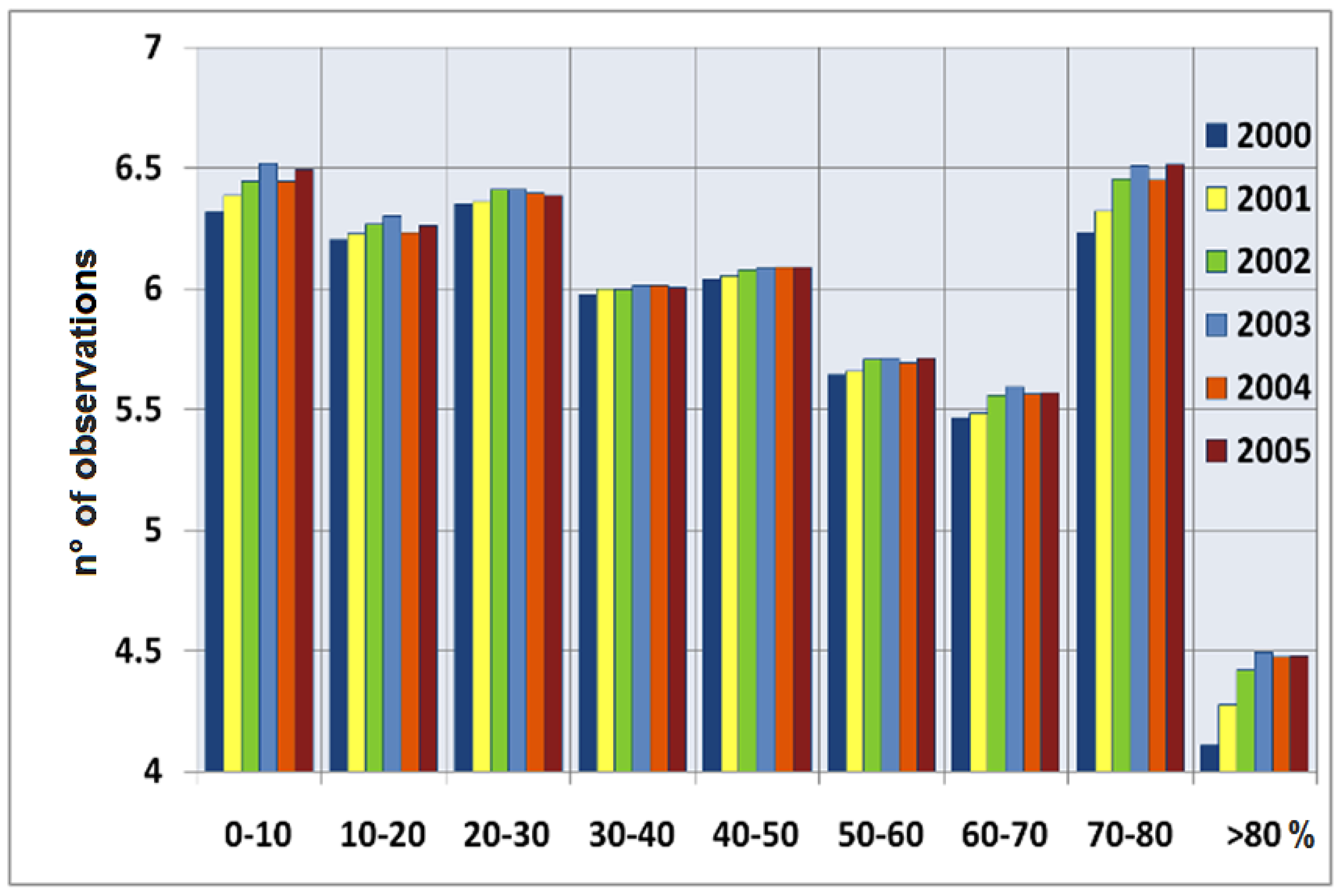
3.2. 2000 to 2005 South America Biomass Burning

In South America, biomass burning presents spatial and temporal variability, associated directly with LULC management. The highest incidences of fires are located in the arc of deforestation, in the Amazon forest border. Therefore, the greatest incidence of fires can be found in areas of vegetation composed mainly of broadleaved evergreen or semi-deciduous forest, representing approximately 39% of 2005 fires; this is followed by herbaceous vegetation (grassland, savannas or lichens/mosses) with 16.6% of 2005 fires; mosaic vegetation (grassland/shrubland/forest)/cropland; mosaic cropland/vegetation (grassland/shrubland/forest) with approximately 9% of 2005 fires; and cropland areas (6.4%). Table 2 shows the LULC for South America and its percentage of 2005 fires presented in each class.
Table 2. GLOBCOVER LULC and the percentage of 2005 fires presented in each class.
GLOBCOVER LULC(%)
26.4
37.8
49.3
538.9
63.8
7
11
0.5
3.2
121.5
1316.6
142.0
153.3
161.6
170.1
181.4
190.1
203.1
220.4
Figure 7 shows the annual (2000 to 2005) accumulative fire pixels that occur in each VCF tree cover classes (y-axis in logarithm of base 10). We notice that most of South America’s biomass burning is located in VCF tree cover classes of 0–10%, 20–30% and 70–80%, corresponding approximately to 15%, 13% and 17% of total fire pixel counts, respectively. Also, this figure shows a propensity to increasing the number of fire focus in all VCF classes, mainly in VCF values greater than 70, that represents biomes with a high quantity of biomass. When comparing 2005 to 2000, we notice that biomass burning increased in areas of Broadleaved evergreen or semi-deciduous forest and savannah regions. These areas are composed mainly of Amazon Forest biome and Brazilian Cerrado (savannah biome). Also, the highest increase occurs in vegetation with continuous field tree cover greater than 70–80% due the deforestation expansion. These results are consistent with evaluation using GLOBCOVER LULC, since the highest incidence of fires, approximately 34%, occurs in pixel area occupied by woody vegetation with VCF values greater than 60%, referring to evergreen broadleaf forest, deciduous broadleaf forest and mixed forest. Also, the same pattern was found to grasslands and herbaceous vegetation with approximately 27% of fires in VCF classes less than 30%.
Figure 7. Incidence of annual fires (2000 to 2005), derived from MODIS and GOES products to South America, in each VCF tree cover class (values are in logarithm base 10).
Remotesensing 03 02110 g007
Figure 8. Distribution of FRP (in 106 watts, or MW), derived from MODIS and GOES products to South America (2000 to 2005), showing the annual variation of fire intensity (y-axis in logarithm base 10).
Remotesensing 03 02110 g008
Figure 8 shows the annual fire radiative power released per pixel as retrieved from MODIS and GOES fire products separated in intervals of 1,000 MW. The FRP values, resampled to a 10 km grid, are composed of a sum of daily FRP released in South America biomass burning season. We notice that the highest annual occurrences of FRP are concentrated in first class (0–1,000 MW). In this class, the number of observations between 2000 and 2005 showed a low variation during all periods, indicating that years with positive or negative rainfall rates do not influence expressively in small fires.
During the studied period (2000 to 2005), Amazon region had negative rainfall anomalies in 2002, 2003 and 2005 and positive rainfall anomalies in 2000, 2001 and 2004. Consequently, as showed in Figure 8, some variations in FRP classes can be attributed to the rainfall anomalies. In the years of high rainfall rate (positive anomaly), the occurrence of intense fires decrease and, as a consequence, FRP values decline significantly. We notice this pattern in reduced number of observations in FRP classes greater than 3,000 MW for 2000 (dark blue), 2001 (light yellow) and 2004 (orange) years compared to years with negative rainfall rate.
Moreover, in dry years the intensity of fires increases significantly such as in 2005, when South America had a negative anomaly rainfall as analyzed by TRMM data (Figure 9). In this year, FRP values showed a significant increase mainly in classes greater than 6,000 MW. The increase in energy released by South American fires could be related to increase of dry biomass and with large fire areas.
Figure 9. 2005 Rainfall Anomaly derived by TRMM 1998–2010 series product; blue color represents positive values of rainfall anomaly and yellow/red colors represent negative rainfall anomaly values.
Remotesensing 03 02110 g009

4. Conclusions

Although GLOBCOVER is a global product, it showed a good agreement in representing South American land use and land cover (LULC). However, like all products derived from automatic classification, some errors are present in the results, such as the overestimation of broadleaved evergreen or semi-deciduous forest and the under-estimation of urban areas and vegetation composed of mangroves. Therefore, to improve the map of vegetation areas and urban areas, we suggest verification using other products derived from satellites, such as the images of City Lights, created with the data from the Defence Meteorological Satellite Program (DMSP).
Concerning the burned areas, it is noticeable that classes with the largest number of fires are related to the Amazon Forest and Cerrado (savannah) biomes and there was a significant increase in the number of fires in areas with a large amount of biomass, resulting therefore in a larger number of emissions of aerosols and trace gases into the atmosphere.

Acknowledgements

The authors acknowledge the financial support from CAPES and FAPESP (2010/07083-0) and to anonymous reviewers for their helpful comments.

References

  1. Kaufman, Y.J.; Justice, C.O.; Flynn, L.; Kendall, J.D.; Prins, E.M.; Giglio, L.; Ward, D.E.; Menzel, W.P.; Setzer, A.W. Potential global fire monitoring from EOS-MODIS. J. Geophys. Res. 1998, 103, 215–238. [Google Scholar] [CrossRef]
  2. Christopher, S.A.; Wang, M.; Berendes, T.A.; Welch, R.M. The 1985 biomass burning season in South America: Satellite remote sensing of fires, smoke and regional radiative energy budget. J. Appl. Meteorol. 1998, 37, 661–678. [Google Scholar] [CrossRef]
  3. Tarasova, T.A.; Nobre, C.A.; Holben, B.N.; Eck, T.F.; Setzer, A. Assessment of smoke aerosol impact on surface solar irradiance measured in the Rondonia region of Brazil during smoke, cloud and radiation—Brazil. J. Geophys. Res. 1999, 104, 161–170. [Google Scholar] [CrossRef]
  4. Tarasova, T.A.; Nobre, C.A.; Holben, B.N.; Eck, T.F.; Setzer, A. Modeling of gaseous, aerosol and cloudiness effects on surface solar irradiance measured in Brazil’s Amazonia 1992–1995. J. Geophys. Res. 2000, 105, 961–969. [Google Scholar] [CrossRef]
  5. Christopher, S.A.; Li, X.; Welch, R.M.; Reid, J.S.; Hobbs, P.V.; Eck, T.F.; Holben, B. Estimation of downward and top-of-atmosphere shortwave irradiances in biomass burning regions during SCAR-B. J. Appl. Meteorol. 2000, 39, 1742–1753. [Google Scholar] [CrossRef]
  6. Li, X.; Christopher, S.A.; Chou, J.; Welch, R.M. Estimation of shortwave direct radiative forcing of biomass burning aerosols using angular dependence models. J. Appl. Meteorol. 2000, 39, 2278–2291. [Google Scholar] [CrossRef]
  7. Wagner, F.; Müller, D.; Ansmann, A. Comparison of the radiative impact of aerosols derived from vertically resolved (lidar) and vertically integrated (Sun photometer) measurements: Example of an Indian aerosol plume. J. Geophys. Res. Atmos. 2001, 106, 22861–22870. [Google Scholar] [CrossRef]
  8. Crutzen, P.J.; Andreae, M.O. Biomass burning in the tropics: Impact on atmospheric chemistry and biogeochemical cycles. Science 1990, 250, 1669–1678. [Google Scholar] [CrossRef] [PubMed]
  9. Fishman, J.; Hoell, J.M.; Bendura, J.R.; Mcneal, R.J.; Kirchhoff, V.W.J.H. NASA GTE TRACE-A experiment (September–October, 1992): Overview. J. Geophys. Res. 1996, 101, 23865–23880. [Google Scholar] [CrossRef]
  10. Reid, J.S.; Hobbs, P.V.; Ferek, R.J. Physical and chemical characteristics of biomass burning aerosol in Brazil. In SCAR-B Proceedings; Transtec: São Paulo, Brazil, 1994; pp. 165–169. [Google Scholar]
  11. Reid, J.S.; Eck, T.F.; Christopher, S.A.; Hobbs, P.; Holben, B. Use of the angstrom exponent to estimate the variability of optical and physical properties of aging smoke particles in Brazil. J. Geophys. Res. 1999, 104, 27473–27490. [Google Scholar] [CrossRef]
  12. Nobre, C.A.; Sellers, P.J.; Shukla, J. Amazonian deforestation and regional climate change. J. Clim. 1991, 4, 957–988. [Google Scholar] [CrossRef]
  13. Nobre, C.A.; Mattos, L.F.; Dereczynski, C.P.; Tarasova, T.A.; Trosnikov, I.V. Overview of atmospheric conditions during the Smoke, Clouds and Radiation-Brazil (SCAR-B) field experiment. J. Geophys. Res. 1998, 103, 809–820. [Google Scholar] [CrossRef]
  14. Kaufman, Y.J.; Tucker, C.J.; Fung, I. Remote sensing of biomass burning in the tropics. J. Geophys. Res. 1990, 95, 9927–9939. [Google Scholar] [CrossRef]
  15. Kaufman, Y.J.; Setzer, A.W.; Ward, D.; Tanré, D.; Holben, B.N.; Menzel, P.; Pereira, M.C.; Rasmussen, R. Biomass Burning And Spaceborne Experiment in the Amazonas (BASE-A). J. Geophys. Res. 1992, 97, 14581–14599. [Google Scholar] [CrossRef]
  16. Riggan, P.J.; Tissell, R.G.; Lockwood, R.N.; Brass, J.A.; Pereira, J.A.R.; Miranda, H.S.; Miranda, A.C.; Campos, T.; Higgins, R. Remote measurement of energy and carbon flux from wildfires in Brazil. Ecol. Appl. 2004, 14, 855–872. [Google Scholar] [CrossRef]
  17. Wooster, M.J.; Roberts, G.; Perry, G.; Kaufman, Y.J. Retrieval of biomass combustion rates and totals from fire radiative power observations: Calibration relationships between biomass consumption and fire radiative energy release. J. Geophys. Res. 2005, 110, D21111:1–D21111:24. [Google Scholar] [CrossRef]
  18. Freeborn, P.H.; Wooster, M.J.; Hao, W.M.; Ryan, C.A.; Nordgren, B.L.; Baker, S.P.; Ichoku, C. Relationships between energy release, fuel mass loss, and trace gas and aerosol emissions during laboratory biomass fires. J. Geophys. Res. 2008, 113. [Google Scholar] [CrossRef]
  19. Ichoku, C.; Kaufman, Y.J. A method to derive smoke emission rates from MODIS fire radiative energy measurements. IEEE Trans. Geosci. Remote Sens. 2005, 43, 2636–2649. [Google Scholar] [CrossRef]
  20. Ichoku, C.; Giglio, L.; Wooster, M.J.; Remer, L.A. Global characterization of biomass-burning patterns using satellite measurements of fire radiative energy. Remote Sens. Environ. 2008, 112, 2950–2962. [Google Scholar] [CrossRef]
  21. Roberts, G.; Wooster, M.J.; Perry, G.; Drake, N.; Rebelo, L.; Dipotso, F. Retrieval of biomass combustion rates and totals from fire radiative power observations: Application to southern Africa using geostationary SEVIRI imagery. J. Geophys. Res. 2005, 110. [Google Scholar] [CrossRef]
  22. Roberts, G.; Wooster, M.J. Fire detection and fire characterization over Africa using Meteosat SEVIRI. IEEE Trans. Geosci. Remote Sens. 2008, 46, 1200–1218. [Google Scholar] [CrossRef]
  23. Vadrevu, K.P.; Ellicott, E.; Badarinath, K.V.S.; Vermote, E. MODIS derived fire characteristics and aerosol optical depth variations during the agricultural residue burning season, north India. Environ. Poll. 2011, 159, 1560–1569. [Google Scholar] [CrossRef] [PubMed]
  24. Henderson-Sellers, A.; Wilson, M.F.; Thomas, G.; Dickinson, R.E. Current Global Land-Surface Data Sets for Use in Climate-Related Studies; Report NCAR/TN. 272; National Center for Atmospheric Research: Boulder, CO, USA, 1986. [Google Scholar]
  25. Defries, R.S.; Townshend, J.R.G. NDVI-derived land cover classifications at a global scale. Int. J. Remote Sens. 1994, 15, 3567–3586. [Google Scholar] [CrossRef]
  26. Loveland, T.R.; Belward, A.S. The IGBP-DIS global 1km land cover data set, DISCover: First results. Int. J. Remote Sens. 1997, 18, 3289–3295. [Google Scholar] [CrossRef]
  27. Hansen, M.C.; Defries, R.S.; Townsend, R.G.; Sohlberg, R. Global land cover classification at 1 km spatial resolution using a classification tree approach. Int. J. Remote Sens. 2000, 21, 1331–1364. [Google Scholar] [CrossRef]
  28. Büttner, G.; Feranec, J.; Jaffrain, G.; Mari, L. The Corine land cover 2000 project. EARSeL eProc. 2004, 3, 331–346. [Google Scholar]
  29. Bartholome, E.; Belward, A. GLC2000: A new approach to global land cover mapping from earth observation data. Int. J. Remote Sens. 2005, 26, 1959–1977. [Google Scholar] [CrossRef]
  30. Arino, O.; Leroy, M.; Ranera, F.; Gross, D.; Bicheron, P.; Nino, F.; Brockman, C.; Defourny, P.; Vancutsem, C.; Achard, F.; et al. The GLOBCOVER Initiative. In Proceedings of the MERIS (A)ATSR Workshop 2005 (ESA SP-597), Frascati, Italy, 26– 30 September 2005.
  31. McCallum, I.; Obersteiner, M.; Nilsson, S.; Shvidenko, A. A spatial comparison of four satellite derived 1 km global land cover datasets. Int. J. Appl. Earth Obs. 2006, 8, 246–255. [Google Scholar] [CrossRef]
  32. Hansen, M.C.; Defries, R.S.; Townshend, J.R.G.; Carroll, M.; Dimiceli, C.; Sohlberg, R.A. Global percent tree cover at a spatial resolution of 500 meters: First results of the MODIS vegetation continuous fields algorithm. Earth Int. 2003, 7, 1–15. [Google Scholar] [CrossRef]
  33. Herold, M.; Mayaux, P.; Woodcock, C.E.; Baccini, A.; Schmullius, C. Challenges in global land cover mapping: An assessment of agreement and accuracy in existing 1 km datasets. Remote Sens. Environ. 2008, 112, 2538–2556. [Google Scholar] [CrossRef]
  34. Latifovic, R.; Olthof, I. Accuracy assessment using sub-pixel fractional error matrices of global land cover products derived from satellite data. Remote Sens. Environ. 2004, 90, 153–165. [Google Scholar] [CrossRef]
  35. Giri, C.; Zhu, Z.; Reed, B. A comparative analysis of the global land cover 2000 and MODIS land cover data sets. Remote Sens. Environ. 2005, 94, 123–132. [Google Scholar] [CrossRef]
  36. Fritz, S.; See, L. Comparison of land cover maps using fuzzy agreement. Int. J. GIS 2005, 19, 787–807. [Google Scholar] [CrossRef]
  37. Neumann, K.; Herold, M.; Hartley, A.; Schmullius, C. Comparative assessment of CORINE2000 and GLC2000: Spatial analysis of land cover data for Europe. Int. J. Appl. Earth Obs. 2007, 9, 425–437. [Google Scholar] [CrossRef]
  38. Bicheron, P.; Defourny, P.; Brockmann, C.; Schouten, L.; Vancutsem, C.; Huc, M.; Bontemps, S.; Leroy, M.; Achard, F.; Herold, M.; et al. GLOBCOVER: Products Description and Validation Report; MEDIAS-France: Toulouse, France, 2009; Available online: http://ionia1.esrin.esa.int/docs/GLOBCOVER_Products_Description_Validation_Report_I2.1.pdf (accessed on 18 November 2009).
  39. Li, M.; Mao, L.; Zhou, C.; Vogelmann, J.E.; Zhu, Z. Comparing forest fragmentation and its drivers in China and the USA with GLOBCOVER v2.2. J. Environ. Manag. 2010, 91, 2572–2580. [Google Scholar] [CrossRef] [PubMed]
  40. Hansen, M.C.; Townshend, J.R.G.; DeFries, R.S.; Carroll, M. Estimation of tree cover using MODIS data at global, continental and regional/local scales. Int. J. Remote Sens. 2005, 26, 4359–4380. [Google Scholar] [CrossRef]
  41. Cartus, O.; Santoro, M.; Schmullius, C.; Li, Z. Large area forest stem volume mapping in the boreal zone using synergy of ERS-1/2 tandem coherence and MODIS vegetation continuous fields. Remote Sens. Environ. 2011, 115, 931–943. [Google Scholar] [CrossRef]
  42. Montesano, P.M.; Nelson, R.; Sun, G.; Margolis, H.; Kerber, A.; Ranson, K.J. MODIS tree cover validation for the circumpolar taiga-tundra transition zone. Remote Sens. Environ. 2009, 113, 2130–2141. [Google Scholar] [CrossRef]
  43. White, M.A.; Shaw, J.D.; Ramsey, R.D. Accuracy assessment of the vegetation continuous field tree cover product using 3954 ground plots in the southwestern USA. Int. J. Remote Sens. 2005, 26, 2699–2704. [Google Scholar] [CrossRef]
  44. Huffman, G.J.; Adler, R.F.; Bolvin, D.T.; Gu, G.; Nelkin, E.J.; Bowman, K.P.; Hong, Y.; Stocker, E.F.; Wolff, D.B. The TRMM multi-satellite precipitation analysis (TMPA): Quasi-global, multiyear, combined-sensor precipitation estimates at fine scale. J. Hydrometeorol. 2007, 8, 38–55. [Google Scholar] [CrossRef]
  45. Pereira, G.; Freitas, S.R.; Moraes, E.C.; Ferreira, N.J.; Shimabukuro, Y.E.; Rao, V.B.; Longo, K.M. Estimating trace gas and aerosol emissions over South America: Relationship between fire radiative energy released and aerosol optical depth observations. Atmos. Environ. 2009, 43, 6388–6397. [Google Scholar] [CrossRef]
  46. Kaufman, Y.J.; Remer, L.A.; Ward, D.E.; Kleidman, R.; Flynn, L.; Shelton, G.; Ottmar, R.D.; Li, R.R.; Fraser, R.S.; McDougal, D. Relationship between remotely sensed fire intensity and rate of emission of smoke: SCAR-C Experiment. In Global Biomass Burning: Atmospheric, Climatic and Biospheric Implications; Levine, J.S., Ed.; MIT Press: Cambridge, MA, USA, 1996; pp. 685–696. [Google Scholar]
  47. Kaufman, Y.J.; Kleidman, R.G.; King, M.D. SCAR-B fires in the tropics: Properties and remote sensing from EOS-MODIS. J. Geophys. Res. 1998, 103, 955–931, 968. [Google Scholar] [CrossRef]
  48. Câmara Neto, G. Modelos, Linguagens e Arquiteturas para Banco de Dados Geográficos. Ph.D. Thesis, Instituto Nacional de Pesquisas Espaciais, São José dos Campos, SP, Brazil, 1995. [Google Scholar]
  49. Hansen, M.C.; Reed, B. A comparison of the IGBP DISCover and University of Maryland 1 km global land cover products. Int. J. Remote Sens. 2000, 21, 1365–1374. [Google Scholar] [CrossRef]
  50. Moody, A.; Woodcock, C.E. Scale-dependent errors in the estimation of land-cover proportions—Implications for global land-cover datasets. Photogramm. Eng. Remote Sens. 1994, 60, 585–594. [Google Scholar]
  51. Latifovic, R.; Olthof, I. Accuracy assessment using sub-pixel fractional error matrices of global land cover products derived from satellite data. Remote Sens. Environ. 2004, 90, 153–165. [Google Scholar] [CrossRef]
  52. Loveland, T.R.; Reed, B.C.; Brown, J.F.; Ohlen, D.O.; Zhu, Z.; Yang, L.; Merchant, J.W. Development of a global land cover characteristics database and IGBP DISCover from 1 km AVHRR data. Int. J. Remote Sens. 2000, 216, 1303–1330. [Google Scholar] [CrossRef]

