Analysis of Incidence Angle and Distance Effects on Terrestrial Laser Scanner Intensity: Search for Correction Methods

Abstract
:1. Introduction
2. TLS Data and Samples

| Data | Instrument (see Table 2) | Reference | Samples |
|---|---|---|---|
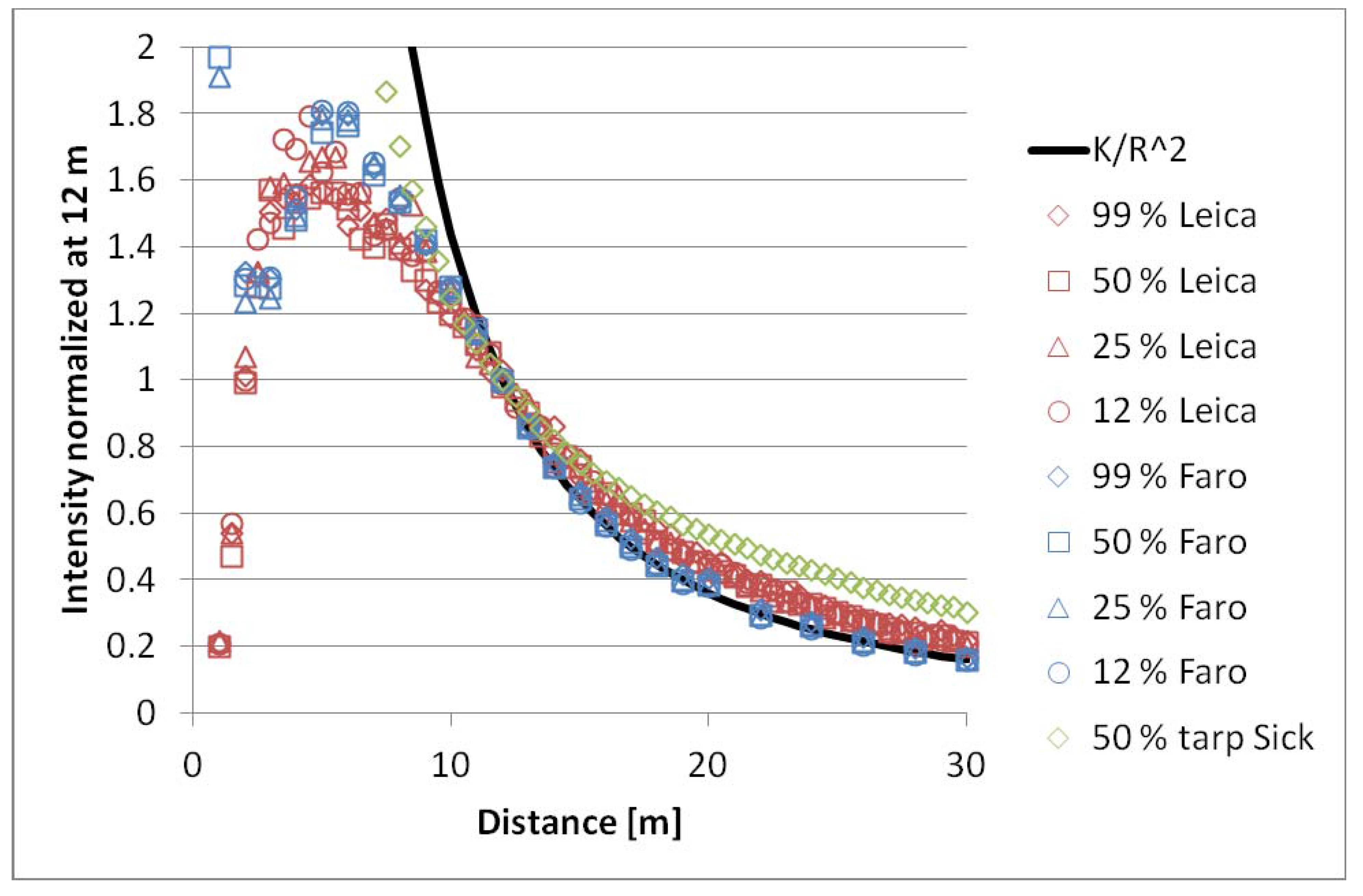
| Intensity vs. range | FARO LS 880HE80 | [13] | 4-step Spectralon target |
| Intensity vs. range | Leica HDS 6100 | [13] | 4-step Spectralon target |
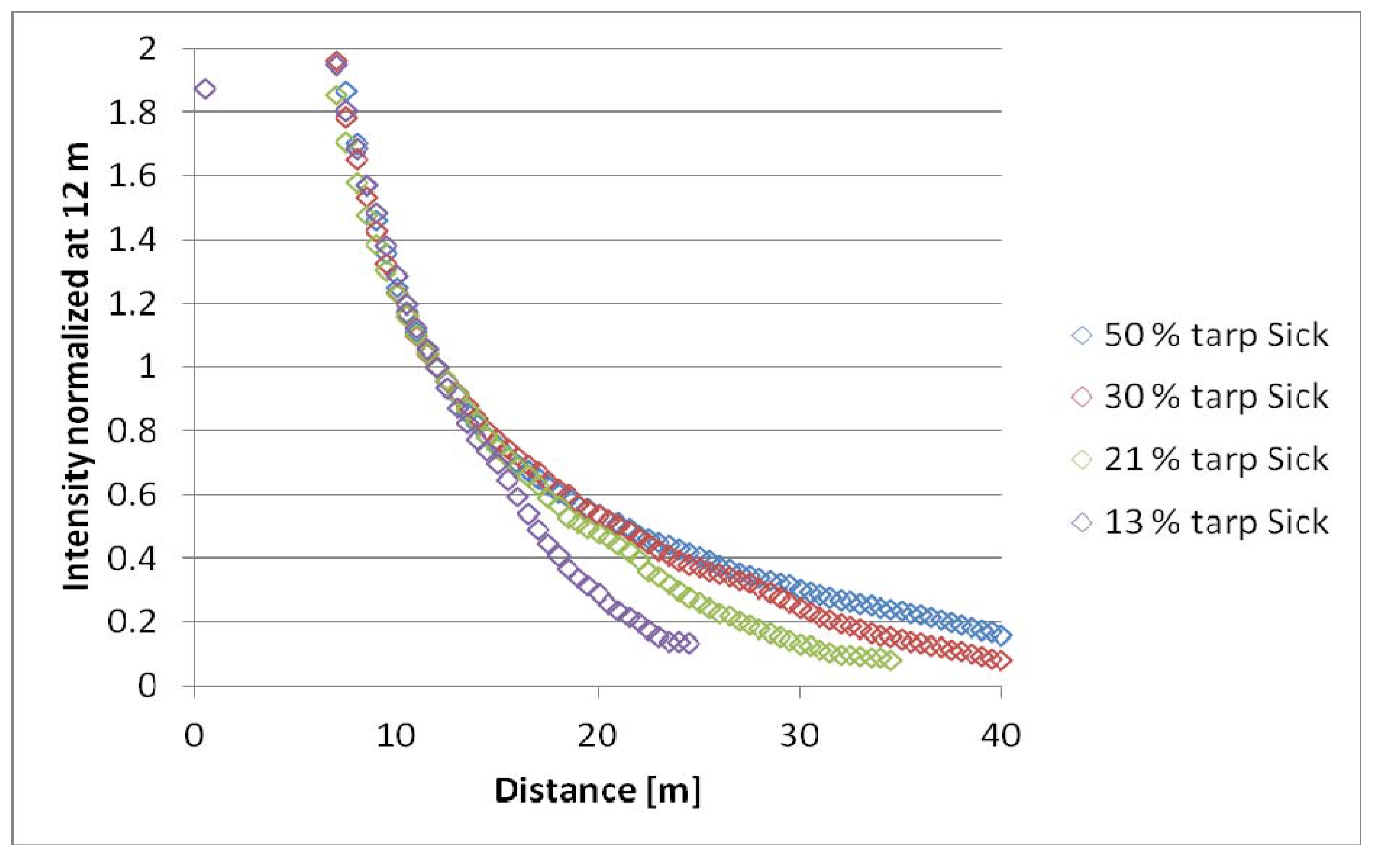
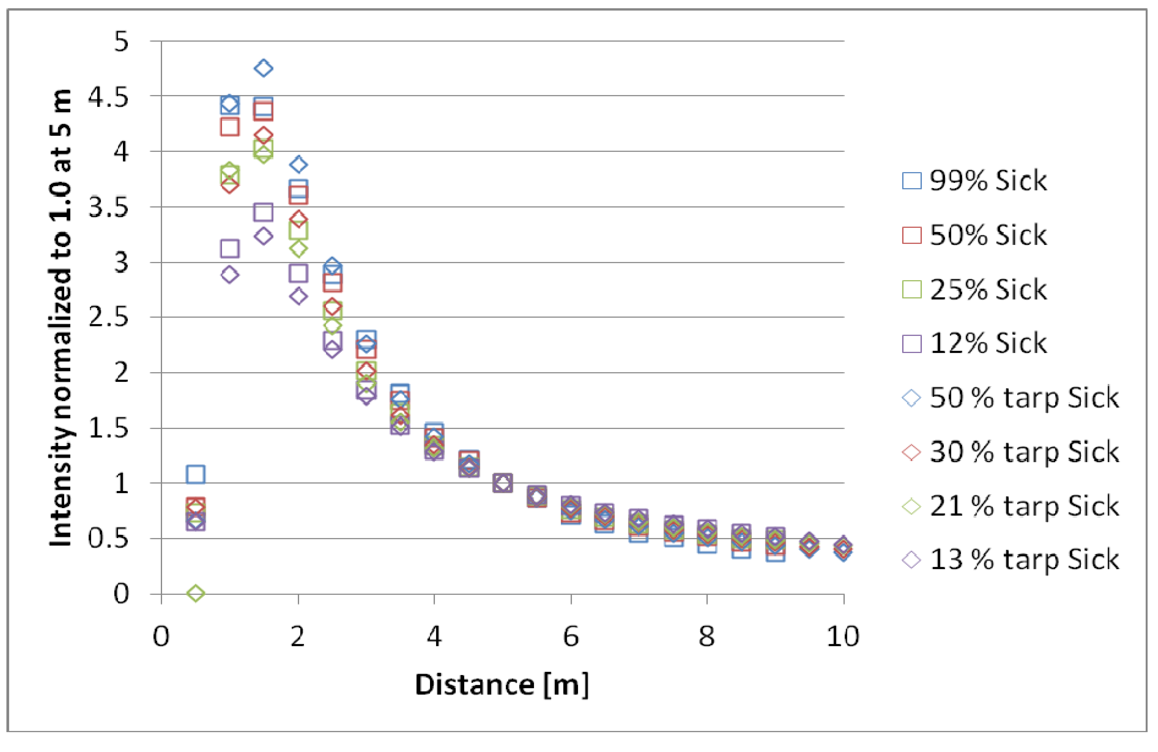
| Intensity vs. range | Sick LMS151 | New data | 4-step Spectralon, brightness tarps |
| Intensity vs. incidence angle | FARO LS 880HE80 | [28] | Brightness tarps, sand & gravel |
| FARO LS 880HE80 | Leica HDS6100 | Sick LMS151 | |
|---|---|---|---|
| Wavelength | 785 nm | 650–690 nm | 905 nm |
| Unambiguity range | 76 m | 79 m | 50 m |
| Field-of-view | 360° × 320° | 360° × 310° | 270° |
| Beam diameter | 3 mm | 3 mm | 8 mm |
| Beam divergence | 0.25 mrad | 0.22 mrad | 15 mrad |
3. The Distance and Incidence Angle Effects
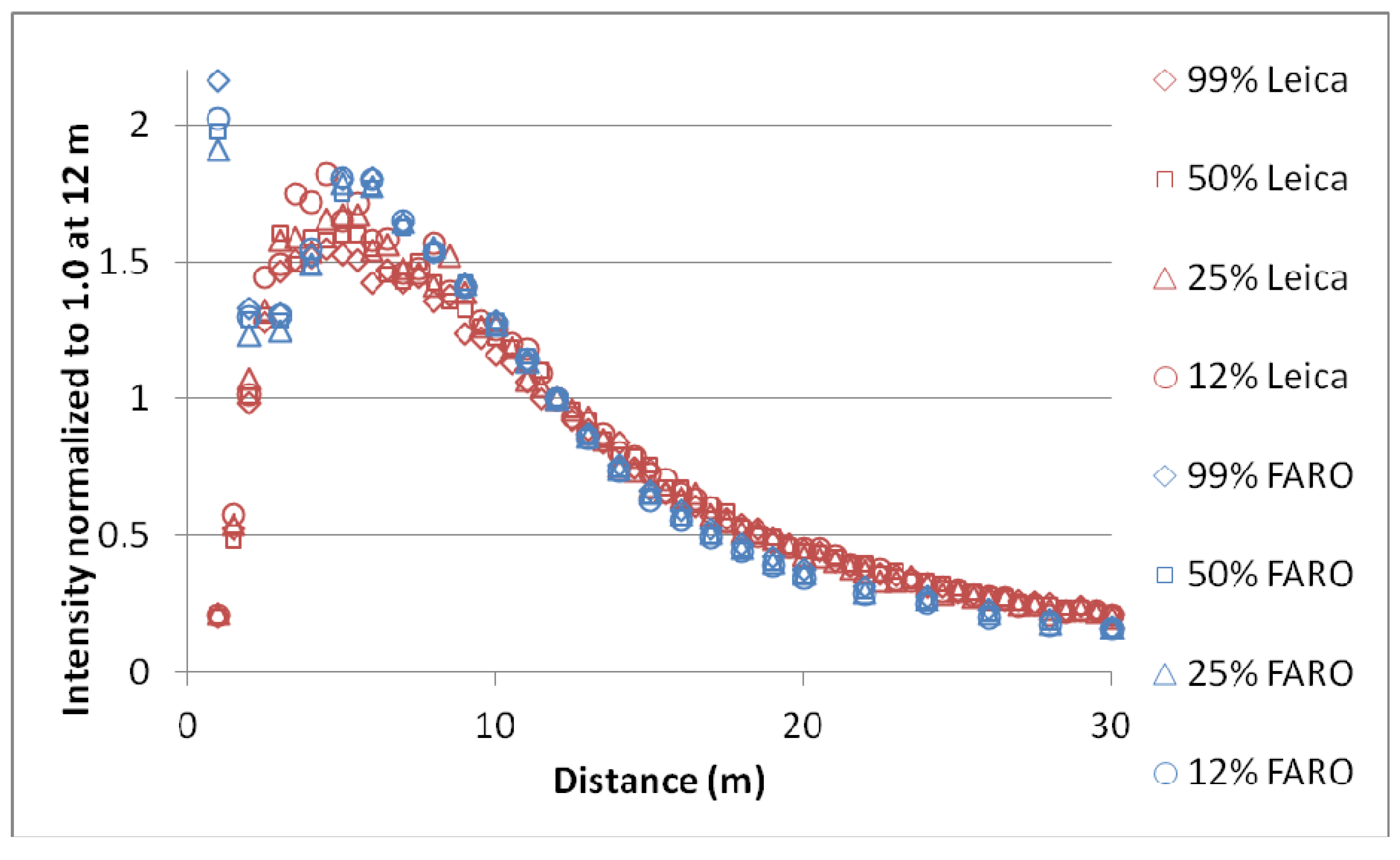
3.1. The Distance Effect
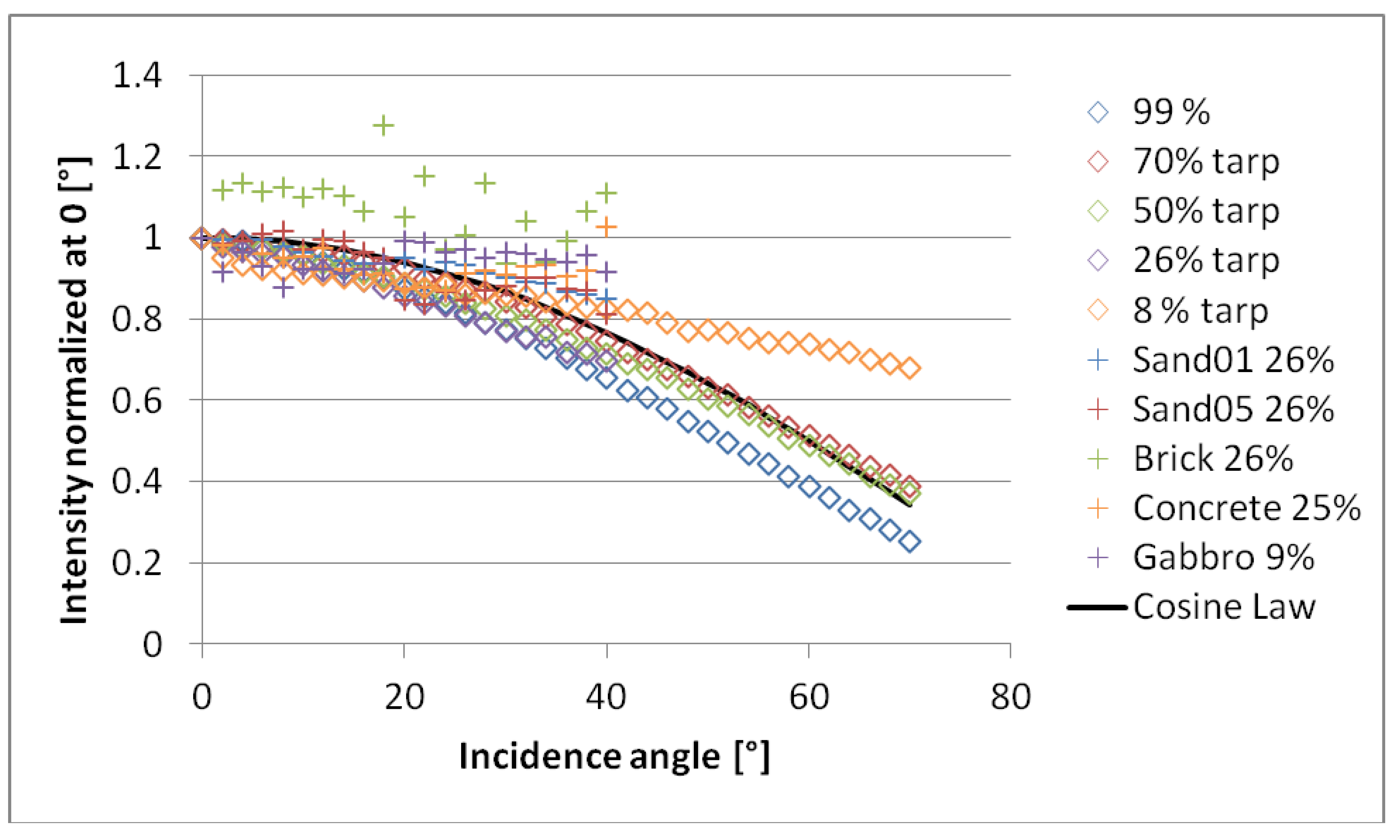
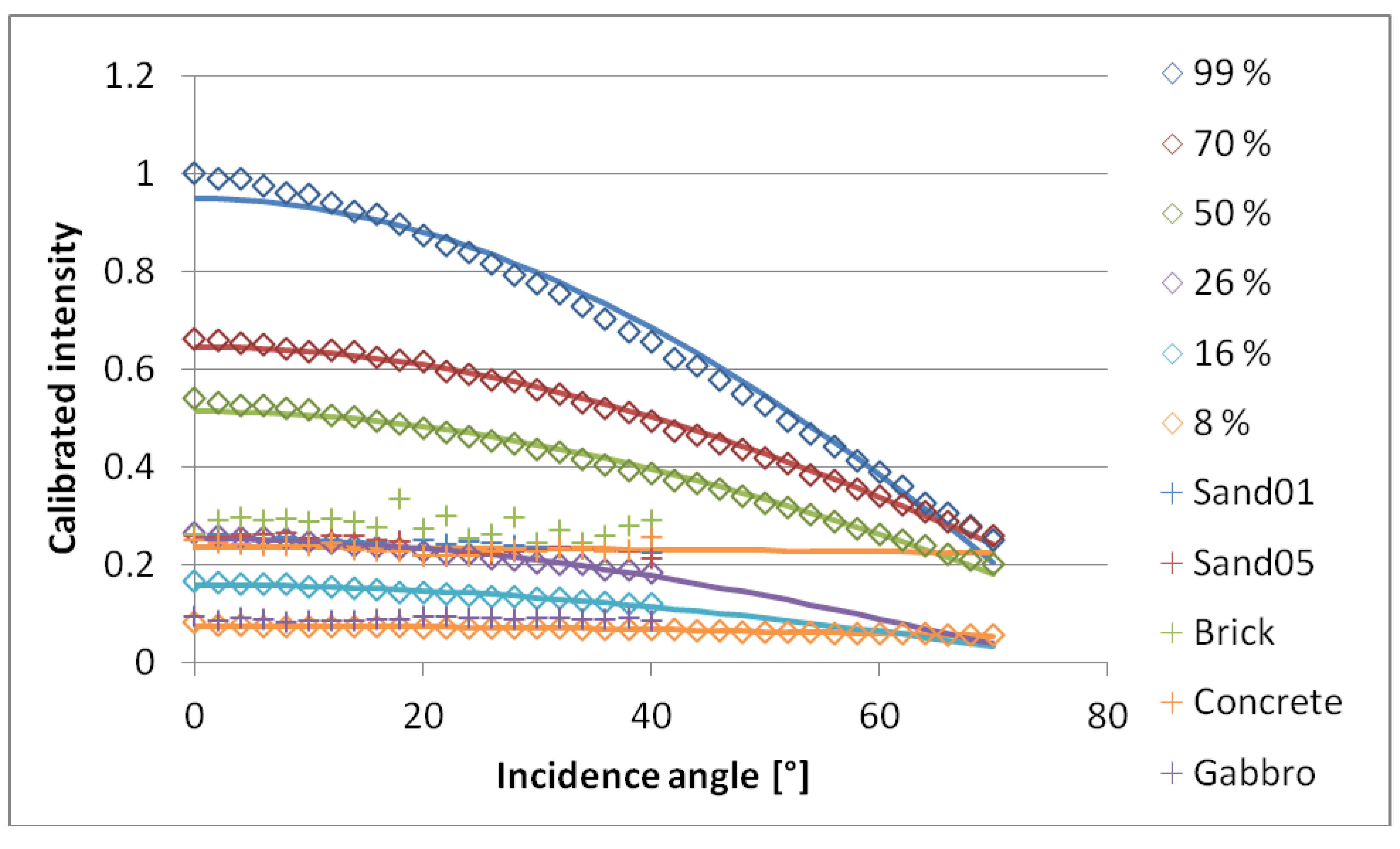
3.2. The Effect of Incidence Angle


| Target | a in Equation (6) | b in Equation (6) |
|---|---|---|
| Spectralon 99% | 0.95 | 1.19 |
| Tarp 70% | 0.65 | 0.95 |
| Tarp 50% | 0.51 | 0.98 |
| Tarp 26% | 0.25 | 1.29 |
| Tarp 16% | 0.16 | 1.19 |
| Tarp 8% | 0.076 | 0.42 |
| Sand (0.1–0.6 mm) | 0.26 | 0.59 |
| Sand (0.5–1.2 mm) | 0.26 | 0.71 |
| Concrete sand (1–5 mm) | 0.24 | 0.08 |
| Gabbro (2–5 mm) | 0.09 | -0.06 |
| Crushed Brick (10–20 mm) | 0.29 | 0.37 |
4. Discussion
5. Conclusions
Acknowledgements
References and Notes
- Jelalian, A.V. Laser Radar Systems; Artech House: Norwood, NJ, USA, 1992; pp. 3–10. [Google Scholar]
- Wagner, W.; Ullrich, A.; Ducic, V.; Melzer, T.; Studnicka, N. Gaussian decomposition and calibration of a novel small-footprint full-waveform digitising airborne laser scanner. ISPRS J. Photogramm. 2006, 60, 100–112. [Google Scholar] [CrossRef]
- Höfle, B.; Pfeifer, N. Correction of laser scanning intensity data: Data and model-driven approaches. ISPRS J. Photogramm. 2007, 62, 415–433. [Google Scholar] [CrossRef]
- Kaasalainen, S.; Hyyppä, H.; Kukko, A.; Litkey, P.; Ahokas, E.; Hyyppä, J.; Lehner, H.; Jaakkola, A.; Suomalainen, J.; Akujärvi, A.; Kaasalainen, M.; Pyysalo, U. Radiometric calibration of LIDAR intensity with commercially available reference targets. IEEE Trans. Geosci. Remote Sens. 2009, 47, 588–598. [Google Scholar] [CrossRef]
- Wagner, W. Radiometric calibration of small-footprint full-waveform airborne laser scanner measurements: Basic physical concepts. ISPRS J. Photogramm. 2010, 65, 505–513. [Google Scholar] [CrossRef]
- Lehner, H.; Briese, C. Radiometric Calibration of Full-Waveform Airborne Laser Scanning Data Based on Natural Surfaces. In Proceedings of ISPRS Technical Commission VII Symposium, 100 Years ISPRS, Advancing Remote Sensing Science, Vienna, Austria, 5–7 July 2010; In IAPRS. 2010; Volume 38, pp. 360–365. [Google Scholar]
- Pfeifer, N.; Höfle, B.; Briese, C.; Rutzinger, M.; Haring, A. Analysis of the Backscattered Energy in Terrestrial Laser Scanning Data. In Proceedings of ISPRS Congress, Beijing, China, 7–11 July 2008; In IAPRS. 2008; Volume 37, pp. 1045–1052. [Google Scholar]
- Béland, M.; Widlowski, J.-L.; Fournier, R.A.; Côté, J.-F.; Verstraete, M.M. Estimating leaf area distribution in savanna trees from terrestrial LiDAR measurements. Agric. Forest Meteorol. 2011, 151, 1252–1266. [Google Scholar] [CrossRef]
- Franceschi, M.; Teza, G.; Preto, N.; Pesci, A.; Galgaro, A.; Girardi, S. Discrimination between marls and limestones using intensity data from terrestrial laser scanner. ISPRS J. Photogramm. 2009, 64, 522–528. [Google Scholar] [CrossRef]
- Burton, D.; Dunlap, D.B.; Wood, L.J.; Flaig, P.P. Lidar intensity as a remote sensor of rock properties. J. Sediment. Res. 2011, 81, 339–347. [Google Scholar] [CrossRef]
- Nield, J.M.; Wiggs, G.F.S.; Squirrell, R.S. Aeolian sand strip mobility and protodune development on a drying beach: examining surface moisture and surface roughness patterns measured by terrestrial laser scanning. Earth Surf. Proc. Land. 2011, 36, 513–522. [Google Scholar] [CrossRef]
- Kaasalainen, S.; Kukko, A.; Lindroos, T.; Litkey, P.; Kaartinen, H.; Hyyppä, J.; Ahokas, E. Brightness measurements and calibration with airborne and terrestrial laser scanners. IEEE Trans. Geosci. Remote Sens. 2008, 46, 528–534. [Google Scholar] [CrossRef]
- Kaasalainen, S.; Krooks, A.; Kukko, A.; Kaartinen, H. Radiometric calibration of terrestrial laser scanners with external reference targets. Remote Sens. 2009, 1, 144–158. [Google Scholar] [CrossRef]
- Balduzzi, M.A.F.; Van der Zande, D.; Stuckens, J.; Verstraeten, W.W.; Coppin, P. The properties of terrestrial laser system intensity for measuring leaf geometries: A case study with conference pear trees (Pyrus Communis). Sensors 2011, 11, 1657–1681. [Google Scholar] [CrossRef] [PubMed]
- Lichti, D.D. Modelling of Laser Scanner NIR Intensity for Multi-Spectral Point Cloud Classification. In Proceedings of Optical 3D Measurement Techniques VI, Zürich, Switzerland, 22–25 September 2003; pp. 282–289.
- Eitel, J.U.H.; Vierling, L.A.; Long, D.S. Simultaneous measurements of plant structure and chlorophyll content in broadleaf saplings with a terrestrial laser scanner. Remote Sens. Environ. 2011, 115, 628–635. [Google Scholar] [CrossRef]
- Voegtle, T.; Wakaluk, S. Effects on the Measurements of the Terrestrial Laser Scanner HDS 6000 (Leica) Caused by Different Object Materials. In Proceedings of Laserscanning 2009, Paris, France, 1–2 September 2009; In IAPRS. 2009; Volume 38, pp. 68–74. [Google Scholar]
- Soudarissanane, S.; Lindenbergh, R.; Menenti, M.; Teunissen, P. Incidence Angle Influence on the Quality of Terrestrial Laser Scanning Points. In Proceedings of Laserscanning 2009, Paris, France, 1–2 September 2009; In IAPRS. 2009; Volume 38, pp. 83–88. [Google Scholar]
- Pesci, A.; Teza, G. Effects of surface irregularities on intensity data from laser scanning: An experimental approach. Ann. Geophys. 2008, 51, 839–848. [Google Scholar]
- Jaakkola, A.; Hyyppä, J.; Hyyppä, H.; Kukko, A. Retrieval algorithms for road surface modelling based on mobile mapping. Sensors 2008, 8, 5238–5249. [Google Scholar] [CrossRef]
- Alho, P.; Kukko, A.; Hyyppä, H.; Kaartinen, H.; Hyyppä, J.; Jaakkola, A. Application of boat-based laser scanning for river survey. Earth Surf. Proc. Land. 2009, 34, 1831–1838. [Google Scholar] [CrossRef]
- Kaasalainen, S.; Vain, A.; Krooks, A.; Kukko, A. Topographic and Distance Effects in Laser Scanner Intensity Correction. In Proceedings of Laserscanning 2009, Paris, France, 1–2 September 2009; In IAPRS. 2009; Volume 38, pp. 219–223. [Google Scholar]
- Jutzi, B.; Gross, H. Normalization of LiDAR Intensity Data Based on Range and Surface Incidence Angle. In Proceedings of Laserscanning 2009, Paris, France, 1–2 September 2009; In IAPRS. 2009; Volume 38, pp. 213–218. [Google Scholar]
- Lichti, D.D. Spectral filtering and classification of terrestrial laser scanner point clouds. Photogramm. Rec. 2005, 20, 218–240. [Google Scholar] [CrossRef]
- Hodge, R.; Brasington, J.; Richards, K. In situ characterization of grain-scale fluvial morphology using terrestrial laser scanning. Earth Surf. Proc. Land. 2009, 34, 954–968. [Google Scholar]
- Rees, W.G.; Arnold, N.S. Scale-dependent roughness of a glacier surface: Implications for radar backscatter and aerodynamic roughness modelling. J. Glaciol. 2006, 52, 214–222. [Google Scholar] [CrossRef]
- Egli, L.; Jonas, T.; Grünewald, T.; Schirmer, M.; Burlando, P. Dynamics of snow ablation in a small Alpine catchment observed by repeated terrestrial laser scans. Hydrol. Process. 2011, in press. [Google Scholar] [CrossRef]
- Kukko, A.; Kaasalainen, S.; Litkey, P. Effect of incidence angle on laser scanner intensity and surface data. Appl. Opt. 2008, 47, 986–992. [Google Scholar] [CrossRef] [PubMed]
- Labsphere Inc. Reflectance Materials and Coatings, Technical Guide; Labsphere Inc.: North Sutton, NH, USA; Available online: http://www.labsphere.com/uploads/technical-guides/a-guide-to-reflectance-materials-and-coatings.pdf (accessed on 19 October 2011).
- Jaakkola, A.; Kaasalainen, S.; Hyyppä, J.; Niittymäki, H.; Akujärvi, A. Intensity Calibration and Imaging with SwissRanger SR-3000 Range Camera. In Proceedings of the ISPRS Congress Beijing 2008, Beijing, China, 3–11 July 2008; In IAPRS. 2008; Volume 36, pp. 155–159. [Google Scholar]
- Pfennigbauer, M.; Ullrich, A. Improving quality of laser scanning data acquisition through calibrated amplitude and pulse deviation measurement. Proc. SPIE 2010. [Google Scholar] [CrossRef]
- Hapke, B. Theory of Reflectance and Emittance Spectroscopy; Cambridge University Press: Cambridge, UK, 1993; p. 185. [Google Scholar]
- Kaasalainen, S.; Kaasalainen, M.; Piironen, J. Ground reference for space remote sensing: Laboratory photometry of an asteroid model. Astron. Astrophys. 2005, 440, 1177–1182. [Google Scholar] [CrossRef]
- Kaasalainen, M.; Lamberg, L. Inverse problems of generalized projection operators. Inverse Probl. 2006, 22, 749–769. [Google Scholar] [CrossRef]
- Kaasalainen, S.; Ahokas, E.; Hyyppä, J.; Suomalainen, J. Study of surface brightness from backscattered laser intensity: Calibration of laser data. IEEE Geosci. Remote Sens. Lett. 2005, 2, 255–259. [Google Scholar] [CrossRef]
© 2011 by the authors; licensee MDPI, Basel, Switzerland. This article is an open access article distributed under the terms and conditions of the Creative Commons Attribution license (http://creativecommons.org/licenses/by/3.0/).
Share and Cite
Kaasalainen, S.; Jaakkola, A.; Kaasalainen, M.; Krooks, A.; Kukko, A. Analysis of Incidence Angle and Distance Effects on Terrestrial Laser Scanner Intensity: Search for Correction Methods. Remote Sens. 2011, 3, 2207-2221. https://doi.org/10.3390/rs3102207
Kaasalainen S, Jaakkola A, Kaasalainen M, Krooks A, Kukko A. Analysis of Incidence Angle and Distance Effects on Terrestrial Laser Scanner Intensity: Search for Correction Methods. Remote Sensing. 2011; 3(10):2207-2221. https://doi.org/10.3390/rs3102207
Chicago/Turabian StyleKaasalainen, Sanna, Anttoni Jaakkola, Mikko Kaasalainen, Anssi Krooks, and Antero Kukko. 2011. "Analysis of Incidence Angle and Distance Effects on Terrestrial Laser Scanner Intensity: Search for Correction Methods" Remote Sensing 3, no. 10: 2207-2221. https://doi.org/10.3390/rs3102207