Machine Learning Comparison between WorldView-2 and QuickBird-2-Simulated Imagery Regarding Object-Based Urban Land Cover Classification

Abstract

The objective of this study is to compare WorldView-2 (WV-2) and QuickBird-2-simulated (QB-2) imagery regarding their potential for object-based urban land cover classification. Optimal segmentation parameters were automatically found for each data set and the obtained results were quantitatively compared and discussed. Four different feature selection algorithms were used in order to verify to which data set the most relevant object-based features belong to. Object-based classifications were performed with four different supervised algorithms applied to each data set and the obtained accuracies and model performances indexes were compared. Segmentation experiments carried out involving bands exclusively available in the WV-2 sensor generated segments slightly more similar to our reference segments (only about 0.23 discrepancy). Fifty seven percent of the different selected features and 53% of all the 80 selections refer to features that can only be calculated with the additional bands of the WV-2 sensor. On the other hand, 57% of the most relevant features and 63% of the second most relevant features can also be calculated considering only the QB-2 bands. In 10 out of 16 classifications, higher Kappa values were achieved when features related to the additional bands of the WV-2 sensor were also considered. In most cases, classifications carried out with the 8-band-related features generated less complex and more efficient models than those generated only with QB-2 band-related features. Our results lead to the conclusion that spectrally similar classes like ceramic tile roofs and bare soil, as well as asphalt and dark asbestos roofs can be better distinguished when the additional bands of the WV-2 sensor are used throughout the object-based classification process.

1. Introduction

Presently, the importance of urban studies that can guide more efficient city planning policies has increased in the context of recent massive urban sprawl, climate change and the generally accepted need for environmental protection [1]. One of the most basic data on which urban planning is based is the land cover map of the city, which can be obtained most efficiently with remote sensing data. Nevertheless, visual image interpretation can be very time-consuming and automatic classification approaches proposed by research in the last few years still face some limitations. These limitations are no longer related to the coarse spatial resolution of the sensors, because for the last ten years imagery from several space-borne sensor systems with sub-meter spatial resolution have been available [2]. Obtaining better results is most frequently hampered by the fact that these sensors provide images with only four spectral bands (generally named blue, green, red and infra-red), which makes the distinction of urban land cover classes of similar coloration a difficult task [3,4].

With the launch of the WorldView-2 (WV-2) satellite, for the first time ever, a high spatial resolution space-borne sensor with eight spectral bands ranging from blue to the near infrared parts of the electromagnetic spectrum has been operating [5]. According to its manufacturer, the additional Coastal Blue (400–450 nm), Yellow (585–625 nm), Red-Edge (705–745 nm) and NearIR-2 (860–1,040 nm) bands can provide an increase of up to 30% in the classification accuracy, if compared to analyses performed with only the four multispectral bands also available in sensors like the GeoEye-1, Ikonos or the QuickBird-2 (QB-2) [5]. Due to its greater spatial resolution and higher spectral fidelity, WV-2 images could provide higher potential not only for bathymetric studies and vegetation analysis, but also for the distinction of urban features with similar spectral properties, such as dark coloration roofing and asphalt paved roads [5]. What still has not been studied by researches from the remote sensing community is whether, and to what degree, this last affirmation is true. In this context, the aim of this study is to investigate, based on different machine learning algorithms, whether the WV-2 sensor has indeed a higher potential than the QB-2 sensor for distinguishing spectrally similar urban land cover classes. Our hypothesis is that the great diversity of pavements, roof and vegetation types present in the urban environment, which sometimes have similar colors but different chemical compositions and energy balances with the surroundings, could be more easily and accurately distinguished using the additional bands of the WV-2 sensor throughout the classification routine.

For most urban remote sensing applications and for most of those ones based on very high spatial resolution data, the object-based image analysis approach is advantageous [4,6,7,8,9]. Object-based image classification involves three main steps: (1) determine appropriate segmentation parameters; (2) selection of image and ancillary features to be used in the classification and; (3) definition of classification rules or the application of a classification algorithm [9,10]. Therefore, this investigation on the importance of the WV-2 additional bands regarding urban land cover classification is based on analyses related to each of these different object-based classification steps. The analysis related to the segmentation step tries to answer the questions: “Does the use of the additional WV-2 bands in the segmentation process generate better results?”; and “How important are these new bands in comparison to those present in other sensors?”. Following that, based on automatic feature selection algorithms, we inspect whether specific features related to WV-2 additional bands are more relevant for the distinction of similar urban land cover classes. Lastly, classifications are performed with different algorithms considering features related to all bands of WV-2 and then considering only those features related to the bands available also in the QB-2 sensor system. In relation to our previous study [11], we further discuss here the feature selection results. Additionally, we propose two other analyses in order to compare the potential of the two imagery data sets, namely: the segmentation results quantitative comparison and the classification accuracy and performance comparisons.

2. Methodology

2.1. Study Site and Data Preparation

This study was carried out with a WV-2 image from a section of São Paulo (Brazil). São Paulo is part of a continuous metropolitan area with over 19 million inhabitants [12], where roofs, streets and sidewalk pavements are made of different construction materials such as asbestos, concrete and asphalt. These urban objects are frequently spatially arranged in a dense and complex manner and can be found in different states of conservation. Moreover, despite having similar colorations, these objects have very different chemical compositions and physical properties. Furthermore, no geometrical and contextual pattern is constant in this urban area, which makes even a visual interpretation a difficult task.

As in most urban remote sensing applications with high spatial resolution imagery, an image sharpening procedure was carried out where the spectral information of the eight multispectral bands of the WV-2 sensor was combined with the higher spatial resolution panchromatic band (0.5 m). A Principal Components image sharpening algorithm was used along with the nearest-neighbor re-sampling method, which is the interpolator that changes original spectral signatures the least [13]. As the panchromatic band (450–800 nm) covers a significant part of the entire eight-band spectrum (400–1,040 nm) [3], the pan-sharpening procedure was carried out considering all the eight multispectral bands. Following this, two datasets were created, namely: one with all the eight WV-2 bands and another with only the four bands also available in the QB-2 sensor.

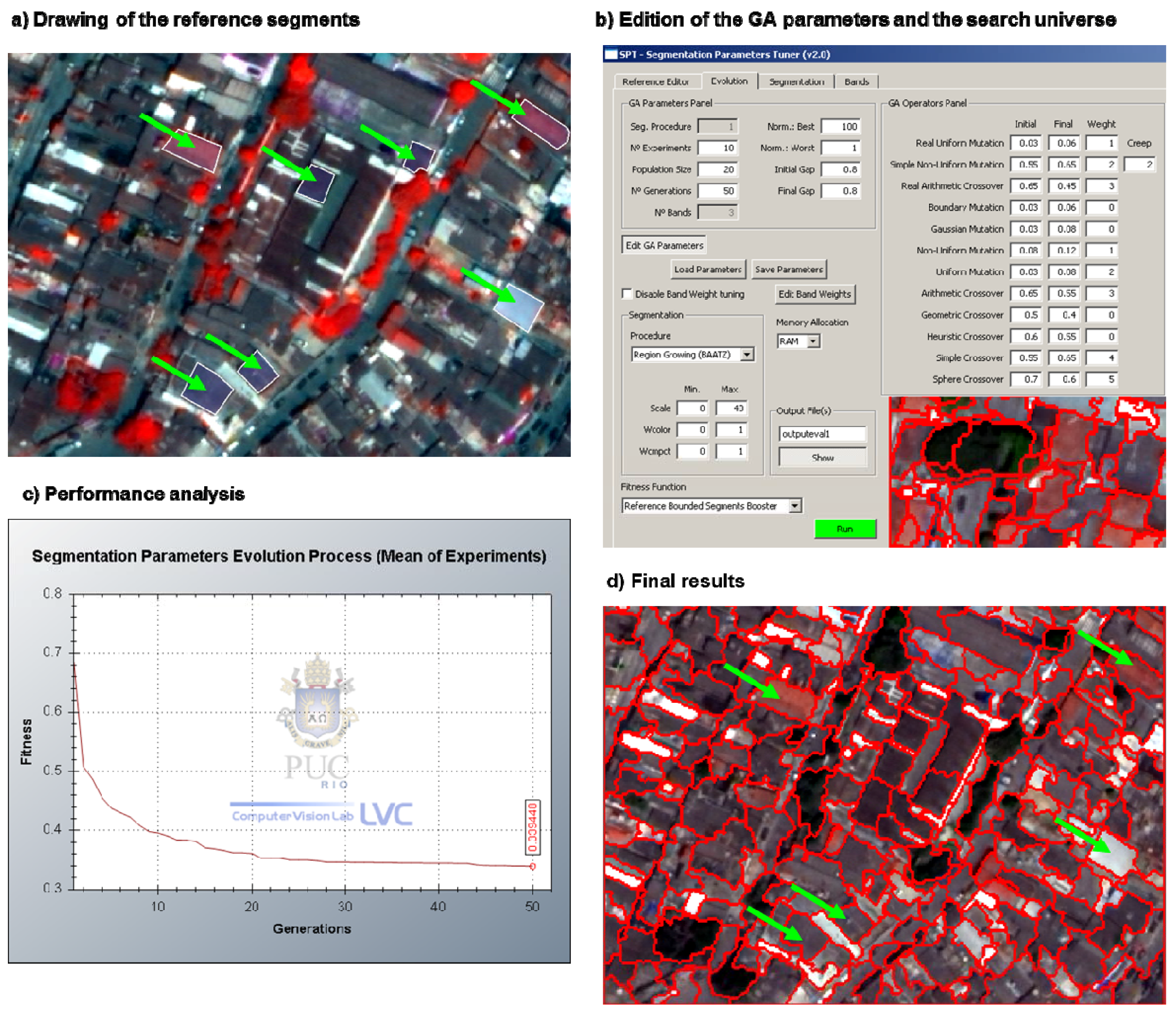
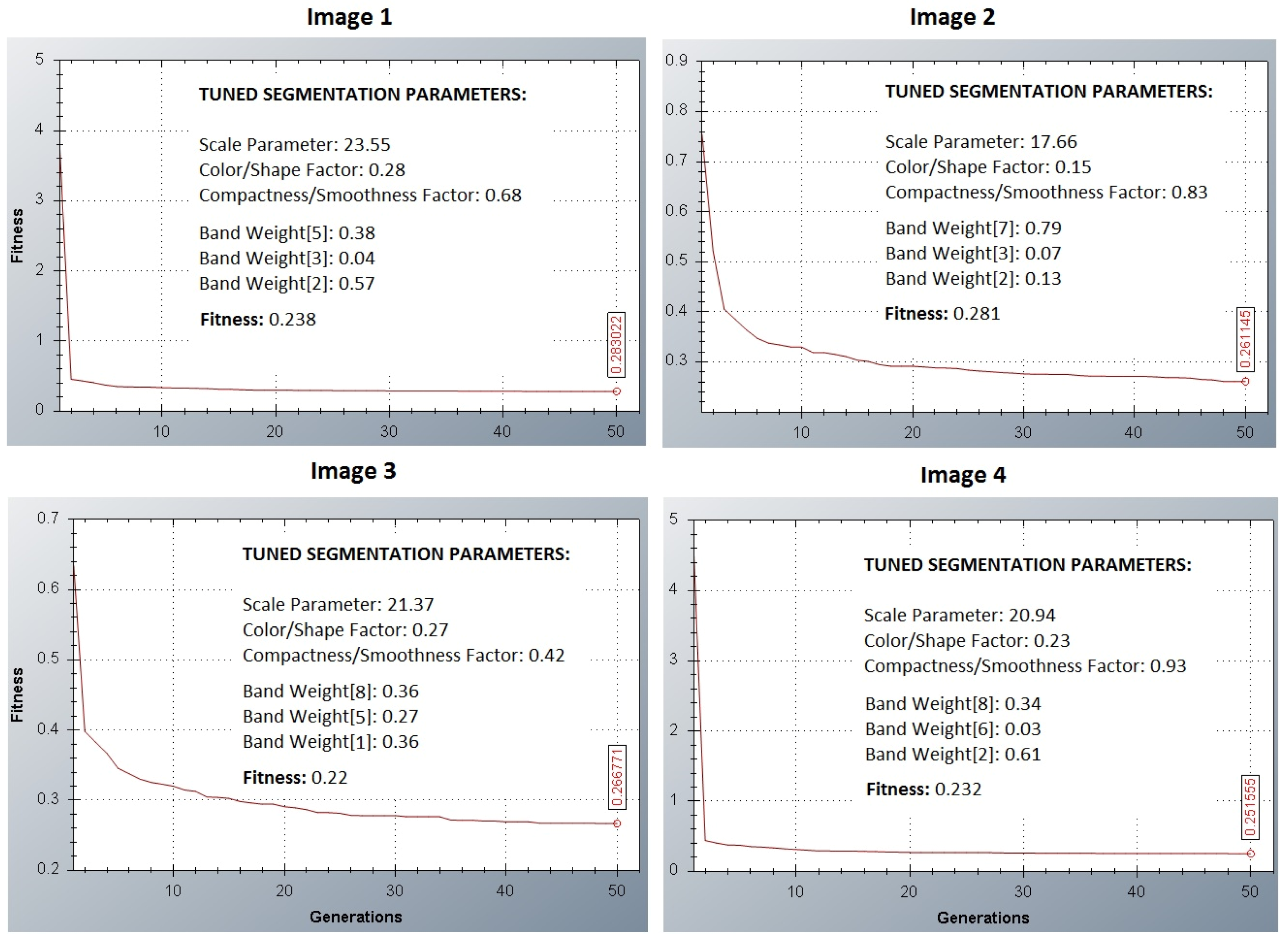
2.2. Segmentation-Based Analysis

One of the objectives of this study is to address the questions: “Does the use of the additional bands of the WV-2 sensor in the segmentation process generate better results?”; and “How important are these new bands in comparison to the ones available in other multispectral sensors?”. Thus, a quantitative evaluation of segmentation results obtained with the WV-2 bands and those obtained only with the bands also available in the QB-2 sensor was conducted using the free-access Segmentation Parameter Tuner system (SPT) [14]. This system uses a Genetic Algorithm (GA) [15] to search for the parameter set that generates segments ideally equal or as similar as possible in shape and size to the reference segments drawn by the user. The system uses a discrepancy measure to evaluate the agreement between the reference segments and the segments generated by each individual of a population (where an individual is a parameter set and a population is a group of different parameter sets). The best individuals from the initial population (which are randomly created) are selected in order to exchange their parameter values among themselves and hence create the next evolved generation of parameter sets. This process runs until the segments match perfectly the reference segments or until the number of generations and experiments is through. The discrepancy measure used in this study to evaluate each individual is called Reference Bounded Segment Booster and it is described by Costa et al. [16], as well as in the SPT’s User Guide [14]. Figure 1 illustrates the process of segmentation parameter search in SPT. Initially, either based on field data, existing cadastral maps or simply image interpretation experience, the user draws the ideal segments over the image (Figure 1(a)). Then, the GA parameters [15] and the procedure parameters (i.e., population size, number of generations and number of experiments) are set and the segmentation algorithm whose parameters will be searched is defined, as well as the search universe (i.e., minimum and maximum possible values of each parameter) (Figure 1(b)). The search universe is set intuitively based on previous experience with the algorithm. When it is not edited, the GA searches the whole possible parameters universe. The end results are the segmented image using the parameter set that enabled the lowest discrepancy with the reference segments and a graph showing the decrease of discrepancy through the evolution of the generations (Figure 1(c,d)).

Our original concept was to submit together the eight bands to the parameters tuning process, leaving to the GA the calibration of the weights (hence, the importance) of the individual bands. However, presently the SPT system only processes images with up to three bands. Therefore, four different three-band images were created, namely:

• Image 1: Bands 2, 3 and 5;
• Image 2: Bands 2, 3 and 7;
• Image 3: Bands 1, 5 and 8;
• Image 4: Bands 2, 6 and 8;

While images 1 and 2 are composed only by bands present in the QB-2 sensor, images 3 and 4 contain also bands exclusively available on WV-2. The selection and grouping of bands into these four three-band images was done considering the correlation matrix of the WV-2 image (Table 1) and selecting low correlated bands to compose each image. Each of the four images was then submitted to a segmentation parameter tuning process using SPT. Some of the GA procedure parameters, as well as the search space defined for all experiments are shown in Table 2. The segmentation algorithm whose parameters were tuned was proposed by Baatz and Schäpe (2000) [17].

Figure 1. Sequence of procedures for the calibration of segmentation parameters using the Segmentation Parameter Tuner (SPT) system. On parts (a) and (b), the reference segments are drawn and the SPT parameters are set. Parts (c) and (d) refer to the final results obtained at the end of the process. Genetic Algorithm (GA).

Figure 1. Sequence of procedures for the calibration of segmentation parameters using the Segmentation Parameter Tuner (SPT) system. On parts (a) and (b), the reference segments are drawn and the SPT parameters are set. Parts (c) and (d) refer to the final results obtained at the end of the process. Genetic Algorithm (GA).

Table 1. Band correlation matrix of the WorldView-2 (WV-2) image of São Paulo (Brazil).

Correlation	Band 1	Band 2	Band 3	Band 4	Band 5	Band 6	Band 7	Band 8
Band 1	1
Band 2	0.990286	1
Band 3	0.974494	0.987039	1
Band 4	0.937438	0.942091	0.965501	1
Band 5	0.915844	0.929299	0.955034	0.984436	1
Band 6	0.766527	0.779873	0.846188	0.885299	0.865134	1
Band 7	0.518168	0.538644	0.620546	0.621782	0.608105	0.897162	1
Band 8	0.498322	0.512075	0.591015	0.606024	0.587367	0.877953	0.981882	1

Table 1. Band correlation matrix of the WorldView-2 (WV-2) image of São Paulo (Brazil).

Correlation	Band 1	Band 2	Band 3	Band 4	Band 5	Band 6	Band 7	Band 8
Band 1	1
Band 2	0.990286	1
Band 3	0.974494	0.987039	1
Band 4	0.937438	0.942091	0.965501	1
Band 5	0.915844	0.929299	0.955034	0.984436	1
Band 6	0.766527	0.779873	0.846188	0.885299	0.865134	1
Band 7	0.518168	0.538644	0.620546	0.621782	0.608105	0.897162	1
Band 8	0.498322	0.512075	0.591015	0.606024	0.587367	0.877953	0.981882	1

If the use of bands available only in WV-2 can indeed provide better segmentation results in terms of delineating urban objects in comparison to segmentation results obtained when using only the bands also available in the QB-2 sensor, then segmentation parameter tuning processes performed with images 3 and 4 would result in obtaining parameter sets that generate segments more similar to the reference segments (i.e., lower discrepancy values). It would also be expected that the experiments with images 3 and 4 would converge at the earlier generations to the parameter sets with lower discrepancy measures and that the WV-2 bands would have a higher weight, concerning the band weight parameters.

Table 2. Genetic algorithm parameters and search space defined for the experiments with images 1 to 4.

GA Procedure Parameters			Search Space
				Min.	Max.
No of experiments	10		Scale parameter	0	40
Population size	20		Weight color	0	1
No of generations	50		Weight compactness	0	1

Table 2. Genetic algorithm parameters and search space defined for the experiments with images 1 to 4.

GA Procedure Parameters			Search Space
				Min.	Max.
No of experiments	10		Scale parameter	0	40
Population size	20		Weight color	0	1
No of generations	50		Weight compactness	0	1

The best parameter sets obtained with the SPT system were tested on the Multi-resolution Segmentation algorithm available in the Definiens Developer 7.0 system [18]. Nevertheless, the obtained segments had shapes and sizes significantly different from those obtained with the Baatz and Schäpe (2000) algorithm implemented in SPT [17]. As the same parameter set generates different segments when applied on SPT and on the Definiens Developer 7.0 systems and because we needed to use the Definiens Developer 7.0 systems for calculating image features (see Section 2.3), we decided to find a parameter set that generates satisfactory segments when applied to the Multi-resolution Segmentation algorithm available in the Definiens Developer 7.0 system. Based on a trial-and-error analysis, the following parameters of the Multi-resolution Segmentation algorithm were defined, namely: weight 1.0 for bands 2, 3 and 5; weight 0.0 for all other bands; scale parameter 40; colour parameter 0.5 and compactness 0.7. The segments obtained this way were considered in the subsequent feature selection analysis.

2.3. Feature Selection

To determine the most relevant features to be used in classification routines is not always an easy task when conventional exploratory analyses are carried out (e.g., scatterplot, histograms, feature values shown in grey levels, etc.). This is especially true when hyper-spectral imagery is used or when object-based image classification is performed. When approaching a classification problem through the object-based method, hundreds or even thousands of object-based spectral and textural features, not to mention geometrical and contextual features, can be created and then used for classification rule generation. When using conventional four-band imagery, e.g., QuickBird, Ikonos etc., the Definiens Developer system automatically creates hundreds of spectral and textural features. Because the WV-2 has twice as many bands compared to these sensors, the number of available features makes a detailed qualitative exploratory analysis of such features a very time-consuming task [19]. This makes the use of feature selection and dimensionality reduction algorithms particularly interesting.

The idea of this analysis was to learn if, according to the feature selection algorithms, features related to the additional bands of the WV-2 sensor are more relevant for the distinction of similar urban land cover classes in comparison to those features related to the bands also available in the QB-2 sensor. Hence, after the segmentation process, 1,140 sample segments belonging to different land cover classes were collected and exported along with 588 spectral and textural features available in the Definiens Developer system. (588 is the number of spectral and textural features which the Definiens Developer system calculated by default after the segmentation process). The samples of the land cover classes were collected in a stratified manner based on image interpretation experience and taking care that samples from the same class were far from each other in order to avoid spatial correlation. Then, the samples were organized in four different land cover class groups. The classes belonging to each group and the number of samples of each class are the following:

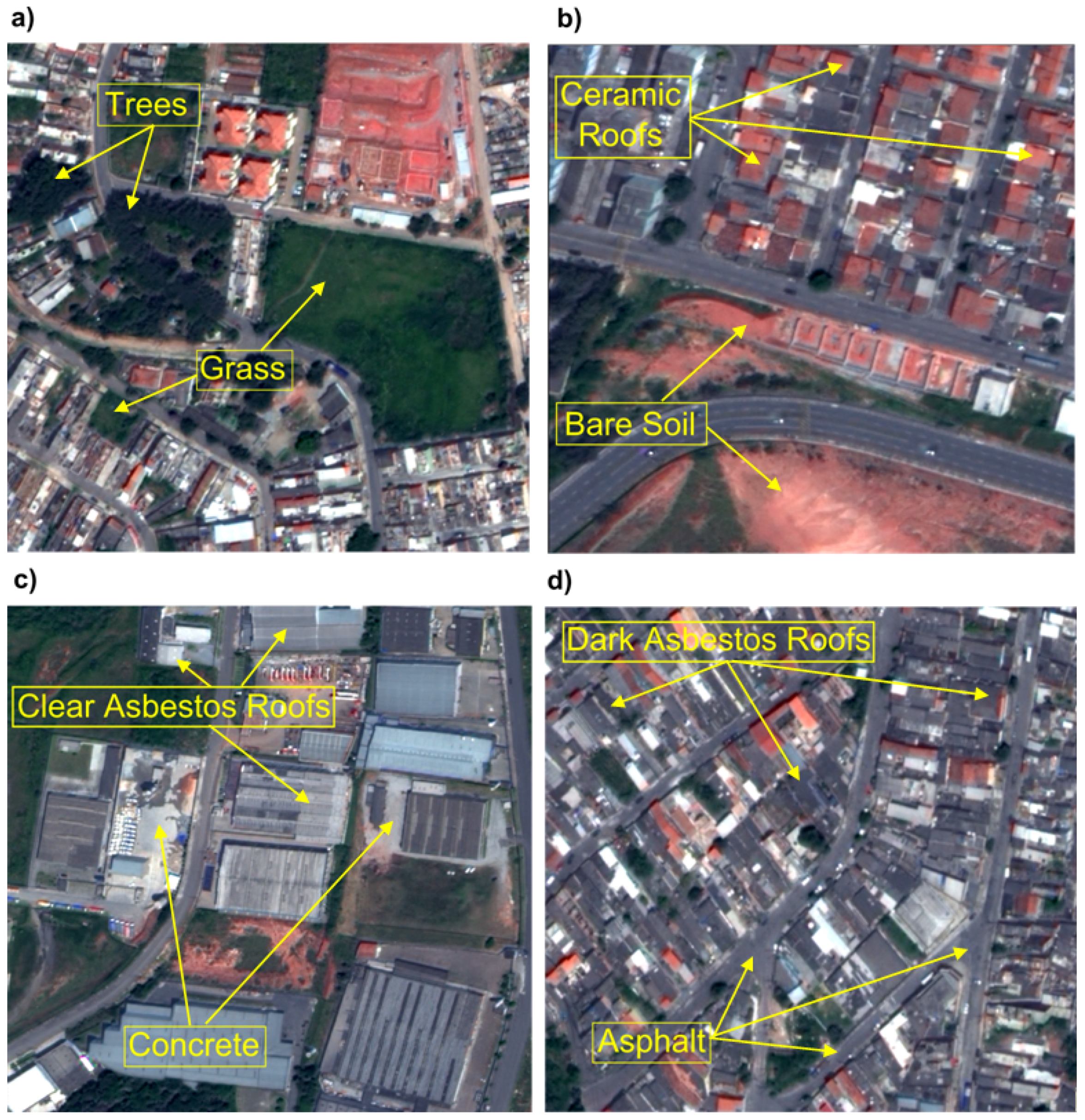
• Group 1 (G1): Grass (311) and Trees (150);
• Group 2 (G2): Ceramic Tile Roofs (151) and Bare Soil (141);
• Group 3 (G3): Concrete (196) and Clear Asbestos Roofs (86);
• Group 4 (G4): Asphalt (53) and Dark Asbestos Roofs (52).

Figure 2 shows sections of the WV-2 image with pointers indicating examples of the land cover classes contained in each of the four groups. Every group contains land cover classes that in many cases can be confused with one another, causing misclassifications and decrease of accuracy [20,21]. The logic in the grouping of the classes is to investigate the distinction of the classes for each group separately.

After the sample grouping, feature selection algorithms were applied on all the collected samples of each group in order to verify which features are most suitable to be used for the distinction of the concerned classes. The feature selection algorithms used in our analysis were: (1) InfoGain [22], which computes the information gain (based on the entropy measure) to evaluate the worth of a feature with respect to the classes; (2) Relief-F [23], which evaluates the value of a feature by repeatedly sampling instances and considering the value of the given feature for the nearest instance(s) of the same and different class(es); (3) Fast Correlation-Based Filter (FCBF) [24], which is based on a correlation measure and relevance/redundancy analysis (this algorithm should be used in conjunction with an attribute set evaluator, in this case, the Symmetrical Uncertainty [24] measure was used); and (4) the Random Forest algorithm [25,26], which is a classification algorithm that also provides a ranking of variable relevance by comparing classification accuracies obtained with, and then without, each of the features. When using the Relief-F (RF) algorithm, the ten nearest neighbors were considered, weighted by their distances to the randomly selected samples in order to calculate class distances. Regarding the RF variable importance calculation algorithm, 100 was the number of trees set to be created by the algorithm. The number of trees was set considering the trade-off between preferable larger forests and processing time. The four algorithms utilized are available at the Weka system, which is a free access and open source data mining and classification software [27]. The extension to this software used for variable importance calculation with the RF algorithm is also available in internet by the link given in the work of Livingston [28]. Only feature selection algorithms which provide a relevance ranking of the features were utilized, because it was intended to discover whether among the best ranked features, those ones related to the bands exclusively available in the WV-2 sensor were present. Furthermore, these algorithms were used because they have different feature evaluation methods to each other and because the descriptions of the algorithms are very well documented in the literature.

Figure 2. Examples of the land cover classes contained in each class group shown in a R(band 5: 630–690 nm), G(band 3: 510–580 nm) and B(band 2: 450–510 nm) color composite of the WV-2 image. (a–d) show the classes of Groups 1–4, respectively.

Figure 2. Examples of the land cover classes contained in each class group shown in a R(band 5: 630–690 nm), G(band 3: 510–580 nm) and B(band 2: 450–510 nm) color composite of the WV-2 image. (a–d) show the classes of Groups 1–4, respectively.

2.4. Land Cover Classification Analysis

We also evaluated the difference in the Kappa index of accuracy [29] between classifications performed, first considering features related to all the eight bands of the WV-2 sensor and then considering only the features related to the bands also available in the QB-2 sensor. Four different classifiers were applied on each data set, namely: (1) Decision Tree by the C4.5 method [4,30]; (2) Random Forest [25,26]; (3) Support Vector Machines [31]; and (4) Regression Tree Classifiers [32,33]. Decision Trees create easy to interpret classification models by hierarchically splitting the data set. Each node of the tree relates to a split in the feature space which is always orthogonal to its axes. The Random Forest classifier consists of a group of decision trees induced with different sub-sets of the training data. Each tree of the forest casts a vote for the class to which a given analysis unit (in this case, a given segment) should be associated. The class with most votes is the one associated to the segment. Support Vector Machines is a sophisticated non-parametric supervised statistical learning technique that finds a hyperplane in the feature space that minimizes misclassifications. Regression Trees differ from Decision Trees in the fact that the earlier uses a multivariate measure to perform tree induction, while the latter uses a univariate measure. When a univariate measure is used for tree induction, the splits are always orthogonal to the feature axis that it refers to (as in the C4.5 Decision Tree algorithm). In this case, every split divides the data according to a certain threshold. On the other hand, when a multivariate measure is used for the tree induction, the splits in the feature space are not orthogonal to its axes because they include linear combination of features, what makes the splits more flexible and better adapted to the distribution of the data on the feature space [22].

Every classifier was applied for each group of classes and on each dataset separately, resulting in 32 individual classifications. The Kappa index was compared, as well as parameters related to the algorithm’s performance. For instance, when applying the Decision Tree classifier, the size of the tree (number of nodes and leaf nodes) was compared. Regarding the Random Tree classifier, the Outof-Bag Error parameter was compared. The number of rules from the Regression Tree classification models was also compared.

For the calculation of the Kappa index of accuracy, one third of the samples available for each class of each group of classes were separated. This means that two thirds of the samples were used for building the model and one third was considered for its validation.

3. Results

3.1. Segmentation Parameters-Based Analysis

Figure 3 shows the best parameter sets obtained with the GA of the SPT for each of the four images, where, as mentioned, images 1 and 2 consist only of bands also present in the QB-2 sensor and images 3 and 4 consist also of bands available exclusively on WV-2. Graphics showing the decrease of discrepancy (increase of agreement between the reference and the produced segments) through the generations is also exhibited in Figure 3. For the four images, the scale, color and compactness parameters are very similar. The optimal scale parameter, regarding the reference segments, is on average 20, while for the color and compactness parameters the average values are approximately 0.23 and 0.71 respectively. The graphics of the segmentation parameters evolution process shows that, for the four cases, the evolution apparently converged to the best achievable parameter sets, meaning that the GA procedure parameters were adequate (Table 2). In case better parameter sets exist, they should be achieved by increasing the mutation parameters of the GA and, at the cost of processing time, the size of the populations and number of generations [15,16].

Regarding the parameters and results comparison between the four images, lower discrepancy values were achieved with images 3 and 4. This may be related to the fact that the bands of images 3 and 4 are least correlated to each other. On the other hand, although its bands are highly correlated, a low discrepancy value was also obtained with image 1. Concerning the band weights, it is surprising that image 3, which obtained the lowest discrepancy value, had band weights more similar to each other in comparison to the other images, where always one of the bands presents very low weights. It is worthwhile to comment that with image 4, the highest weight is that of band 2 (450–510 nm), which is also available on the QB-2 sensor. For the rest, the band weights results do not give clues as to whether the bands not available on the QB-2 play a more important role in the parameter sets. However, based on these results, the use of bands not available in the QB-2 sensor enables slightly better segmentation results.

Figure 3. Results obtained with the Segmentation Parameter Tuner system.

Figure 3. Results obtained with the Segmentation Parameter Tuner system.

3.2. Feature Selection Analysis

Table 3 shows, separately for each of the four groups of classes, only the five most relevant features ranked by each of the feature selection algorithms used in this analysis. The feature names were kept the same as in the Definiens Developer system. The reader is referred to the Reference Book document of this software [18] in order to verify how these features are calculated.

Regarding the selected features, one observes that the four algorithms, which have completely different searching heuristics, selected in all cases more or less the same features (Table 3). In cases of all four groups of classes, the FCBF algorithm selected features which frequently are not present in the selections of the other algorithms. The reason for this is that the FCBF considers not only the relevance of the features but also the redundancy among the most relevant features [24].

Table 3. Results of the analysis from feature selection. R^a stands for the ranking position of the feature and RV^b for the relevance value of the concerned feature. Quick^c indicates a band math feature calculated with only those bands also available in the QB-2 sensor.

Group 1	InfoGain		Relief-F		FCBF		RF
	Ra	RVb	Ra	RVb	Ra	RVb	Ra	RVb
Brightness							4	2.14
Brightness – Quickc					4	0.411
GLDV Ang. 2nd moment Layer 1 (135°)					3	0.473
GLDV Contrast Layer 4 (135°)					5	0.211
Max.pixelvalueLayer3							5	2.14
Mean Layer 3	1	0.824	1	0.309	1	0.906	2	2.83
Mean Layer 4	4	0.728	3	0.224
Min. pixel value Layer 3	2	0.787	2	0.272			1	2.86
Min. pixel value Layer 4	3	0.728	4	0.221	2	0.706
Min. pixel value Layer 5	5	0.661
Min.pixelvalueLayer2							3	2.55
Ratio2 – Quickc			5	0.198
Group 2	InfoGain		Relief-F		FCBF		RF
	Ra	RVb	Ra	RVb	Ra	RVb	Ra	RVb
GLDV Ang. 2nd moment (0°)	4	0.359			3	0.282
GLDV Ang. 2nd moment Layer 8 (all dir.)							3	0.88
GLDV Entropy (0°)							4	0.73
GLDV Entropy Layer 7 (90°)					1	0.317
Mean Layer 3			4	0.102			2	1.01
Min. pixel value Layer 1	5	0.354					5	0.71
Min. pixel value Layer 2	1	0.401	2	0.104	4	0.272
Min. pixel value Layer 3	3	0.379	3	0.103			1	1.24
Ratio Layer 3					5	0.228
Standard deviation Layer 6			5	0.099
Standard deviation Layer 7	2	0.384	1	0.106	2	0.302
Group 3	InfoGain		Relief-F		FCBF		RF
	Ra	RVb	Ra	RVb	Ra	RVb	Ra	RVb
GLCM Correlation Layer 7 (135°)					4	0.118
GLCM StdDev Layer 6 (135°)					3	0.128
GLDV Entropy Layer 4 (45°)					5	0.082
Mean Layer 1					2	0.159
Ratio Layer 1 – Quickc			5	0.124
Ratio Layer 2			2	0.132			3	1.29
Ratio Layer 2 – Quickc	2	0.302
Ratio Layer 3	1	0.311			1	0.413	2	1.32
Ratio Layer 4 – Quickc	3	0.293	4	0.125
Ratio Layer 6							1	1.76
Ratio Layer 7	5	0.293	3	0.126			4	1.27
Ratio Layer 8	4	0.293	1	0.136			5	1.25
Group 4	InfoGain		Relief-F		FCBF		RF
	Ra	RVb	Ra	RVb	Ra	RVb	Ra	RVb
GLCM Dissimilarity (90°)					4	0.223
GLCM Dissimilarity Layer 8 (0°)					5	0.155
Max. Diff.	4	0.385			2	0.223	5	0.29
Max. pixel value Layer 8					3	0.289
Ratio Layer 2 – Quickc	2	0.514	3	0.181			1	0.48
Ratio Layer 3	1	0.536	2	0.209	1	0.155
Ratio Layer 4			5	0.132			4	0.31
Ratio Layer 4 – Quickc	5	0.358	4	0.137			3	0.35
Ratio Layer 8	3	0.503	1	0.269			2	0.47

Table 3. Results of the analysis from feature selection. R^a stands for the ranking position of the feature and RV^b for the relevance value of the concerned feature. Quick^c indicates a band math feature calculated with only those bands also available in the QB-2 sensor.

Group 1	InfoGain		Relief-F		FCBF		RF
	Ra	RVb	Ra	RVb	Ra	RVb	Ra	RVb
Brightness							4	2.14
Brightness – Quickc					4	0.411
GLDV Ang. 2nd moment Layer 1 (135°)					3	0.473
GLDV Contrast Layer 4 (135°)					5	0.211
Max.pixelvalueLayer3							5	2.14
Mean Layer 3	1	0.824	1	0.309	1	0.906	2	2.83
Mean Layer 4	4	0.728	3	0.224
Min. pixel value Layer 3	2	0.787	2	0.272			1	2.86
Min. pixel value Layer 4	3	0.728	4	0.221	2	0.706
Min. pixel value Layer 5	5	0.661
Min.pixelvalueLayer2							3	2.55
Ratio2 – Quickc			5	0.198
Group 2	InfoGain		Relief-F		FCBF		RF
	Ra	RVb	Ra	RVb	Ra	RVb	Ra	RVb
GLDV Ang. 2nd moment (0°)	4	0.359			3	0.282
GLDV Ang. 2nd moment Layer 8 (all dir.)							3	0.88
GLDV Entropy (0°)							4	0.73
GLDV Entropy Layer 7 (90°)					1	0.317
Mean Layer 3			4	0.102			2	1.01
Min. pixel value Layer 1	5	0.354					5	0.71
Min. pixel value Layer 2	1	0.401	2	0.104	4	0.272
Min. pixel value Layer 3	3	0.379	3	0.103			1	1.24
Ratio Layer 3					5	0.228
Standard deviation Layer 6			5	0.099
Standard deviation Layer 7	2	0.384	1	0.106	2	0.302
Group 3	InfoGain		Relief-F		FCBF		RF
	Ra	RVb	Ra	RVb	Ra	RVb	Ra	RVb
GLCM Correlation Layer 7 (135°)					4	0.118
GLCM StdDev Layer 6 (135°)					3	0.128
GLDV Entropy Layer 4 (45°)					5	0.082
Mean Layer 1					2	0.159
Ratio Layer 1 – Quickc			5	0.124
Ratio Layer 2			2	0.132			3	1.29
Ratio Layer 2 – Quickc	2	0.302
Ratio Layer 3	1	0.311			1	0.413	2	1.32
Ratio Layer 4 – Quickc	3	0.293	4	0.125
Ratio Layer 6							1	1.76
Ratio Layer 7	5	0.293	3	0.126			4	1.27
Ratio Layer 8	4	0.293	1	0.136			5	1.25
Group 4	InfoGain		Relief-F		FCBF		RF
	Ra	RVb	Ra	RVb	Ra	RVb	Ra	RVb
GLCM Dissimilarity (90°)					4	0.223
GLCM Dissimilarity Layer 8 (0°)					5	0.155
Max. Diff.	4	0.385			2	0.223	5	0.29
Max. pixel value Layer 8					3	0.289
Ratio Layer 2 – Quickc	2	0.514	3	0.181			1	0.48
Ratio Layer 3	1	0.536	2	0.209	1	0.155
Ratio Layer 4			5	0.132			4	0.31
Ratio Layer 4 – Quickc	5	0.358	4	0.137			3	0.35
Ratio Layer 8	3	0.503	1	0.269			2	0.47

It is also an observable trend that, according to the relevance values of the selected features, classes of group G1 seem to be more separable, followed by those of group G2 and groups G3/G4. In most cases, the selected features are simple statistical or band math spectral features (68 total), instead of textural features (12 total). Among these, the GLDV method [34] computed more relevant features in comparison to the GLCM method [34]. Out of the 80 selections, only 38 refer to features that can also be calculated from a QB-2 image. Furthermore, just 43% of the different selected features were calculated considering bands also available in the QB-2 sensor.

In group G1, the yellow band (585–625 nm) apparently showed potential for vegetation type discrimination (only the RF algorithm did not select a feature related to this band). On the other hand, the mean pixel value of band 3 from the WV-2 system (510–580 nm), which is equivalent to band 2 of QB-2, is definitely the best feature, because it was selected by all four algorithms and ranked first by three of them. Also, none of the first and second places are features that consider any of the additional bands of the WV-2 sensor (bands 1, 4, 6 and 8, which are not available in the QB-2 sensor). When visually inspecting the near infrared images (bands 7 and 8), no strong contrast between Grass and Tree covered areas is observable. In these bands, both classes appear very bright in our study site. This might be the reason why no features related to these bands were selected by the algorithms. Furthermore, out of 12 features selected by the four algorithms considering samples of group G1, only 5 are related to the additional bands of the WV-2 sensor.

Regarding classes of group G2, eight among 11 different selected features are related to bands exclusively available in the WV-2 sensor. Bands 1, 6, 8 and especially band 7, whose related features were the best ranked in the case of algorithms Relief-F and FCBF, are apparently important for the distinction between Bare Soil and Ceramic Tile Roofs, which are classes that in previous urban land cover classifications are reportedly confused among each other [20,21]. It is also worthwhile to stress that this is the group of classes where texture features appeared to be more relevant. Four of the 11 selected features are texture-based. In general, feature Standard deviation layer 7 seems to be very important, considering that it was selected as the first or second most relevant feature by three of the four feature selection algorithms utilized in this analysis.

Considering the classes of group G3, features calculated by dividing the mean value of one band by the sum of the mean value of each of the other bands (Ratio features), are the most relevant ones. Eight of 12 selected features are these so-called Ratio features, calculated either considering all eight bands of WV-2 sensor or only the four bands also present in the QB-2 sensor. The algorithms InfoGain, Relief-F and Random Forest selected only Ratio features. These features, although relevant, may be correlated among each other, which induced the FCBF algorithm to select as third to fifth most pertinent features texture-based ones. Seven out of 12 different selected features are calculated considering all eight bands available. Furthermore, all the first places (best ranked features) consider also the WV-2 additional bands, as well as three of the four second places. It can be inferred from these results that the additional bands of WV-2 have good potential to distinguish the classes Concrete and Clear Asbestos Roofs.

The feature selection results regarding group G4 presented the same trend as group G3 (probably because the classes are spectrally similar), namely: the Ratio features are very pertinent according to the InfoGain, Relief-F and Random Forest algorithms, but, on the other hand, they are probably correlated among each other, which made the FCBF algorithm select other types of features as the second to fifth most pertinent ones. As in the results of group G3, the feature Ratio Layer 3, which is the division of the mean value of band 3 (equivalent to band 2 of the QB-2) by the sum of the mean value from all the eight bands of WV-2, is shown to be the most pertinent one.

Although only 43% of the different selected features and 47% of the eighty selections refer to features that can also be calculated with the QB-2 bands, just 43% of the first places and 37% of the second places refer to features calculated considering the additional bands of the WV-2 sensor.

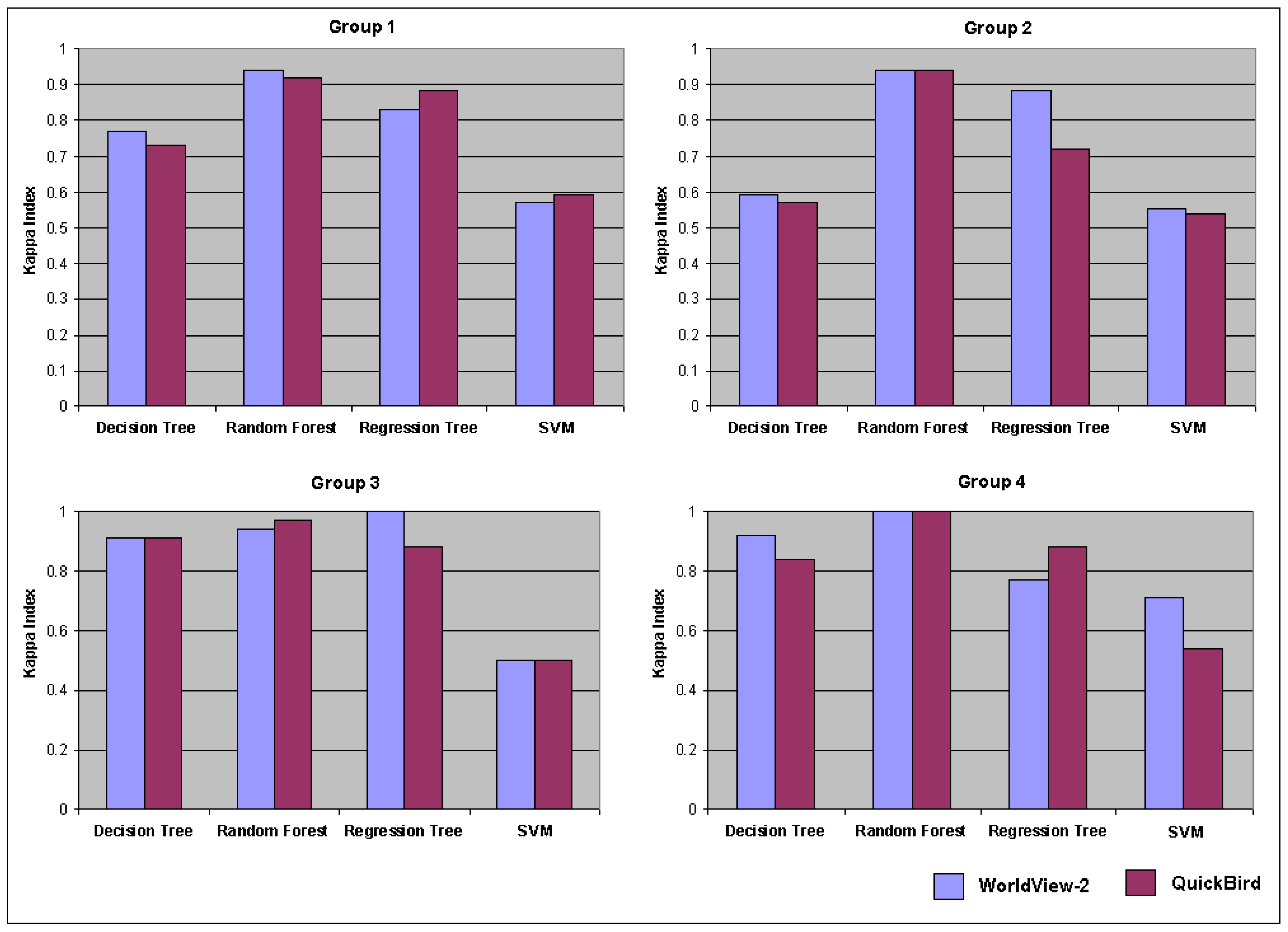
3.3. Classification-Based Analysis

Figure 4 shows the Kappa accuracy results of classifications performed with the different algorithms applied to each group of classes considering first object-based spectral and textural features related to all the eight bands of the WV-2 sensor and then considering only the features related to the bands also present in the QB-2 sensor. The Random Forest was the algorithm whose classifications achieved the highest accuracy values (average of 0.95), followed either by the Regression Tree or the Decision Tree algorithms (averages of 0.85 and 0.77 respectively). One exception is group G3, where the Regression Tree algorithm performed with the full set of features, achieved the highest Kappa index (0.98), overtaking accuracies obtained with the Random Forest algorithm (0.89). In contrast to many other studies [35], the Support Vector Machines classifier performed the worst in all cases (average of 0.57), followed, with the exception of group G4, by the Decision Tree classifier (average of 0.77). The bad performance of the Support Vector Machines classifier may be related to the high dimensionality (588 features) and correlation of the feature space. Because of the fact that the other classifiers evaluate each feature internally, they are less influenced by extensive and correlated feature spaces. Over-fitting of the Support Vector Machines models might also have hampered better results. With groups G1 and G3, the highest accuracy indexes were achieved when considering the features related to all the eight bands of the WV-2 (0.93 and 0.98 respectively), while with groups G2 and G4, the highest accuracy levels were also achieved at classifications performed with features related only to the QB-2 bands (0.94 and 0.98 respectively). In no instance however, did a classification carried out with only the features related to the four bands of QB-2 sensor achieve the highest Kappa value. It should also be emphasized that for the classes of group G2, no algorithm performed better when applied over the smaller group of features. This result is in accordance with the feature selection analysis, which showed that features related to the additional bands of WV-2 sensor seemed to be the most pertinent.

Figure 4. Kappa accuracy index comparison between classifications carried out on each group of classes considering features related to the bands of the WV-2 and QB-2 sensors.

Figure 4. Kappa accuracy index comparison between classifications carried out on each group of classes considering features related to the bands of the WV-2 and QB-2 sensors.

Altogether, it can be concluded from the analysis that, with few exceptions (6 out of 16 classifications), the use of features related to all the bands available on WV-2 is likely to provide higher accuracy index values (although statistical tests were not carried out to attest and measure the accuracy difference between the classifications, as suggested by Fortiel et al. [36]). Despite the fact that the Random Forest algorithm performed best in comparison to the others regarding the Kappa index values, the use of the whole set of features on classifications performed with this algorithm was only advantageous for the classes of group G1 (Kappa of 0.94). The Decision Tree classifier was the algorithm which in three of the four class groups performed better when considering also features related to the additional bands of the WV-2 sensor. This might be related to the fact that the heuristic of this algorithm involves a feature relevance measurement procedure, which bypasses the potential disadvantage of multi-dimensionality. This means that for some of the performed classifications, the availability of more features (those ones related to the additional bands of the WV-2 sensor) and, as the feature selection analysis shown above, not necessarily the more pertinent ones, has probably been a disadvantage instead of an advantage.

Figure 5 shows, for the Decision Tree, Random Forest and Regression Tree classifiers, parameters related to the complexity (in the cases of the Decision and Regression Tree algorithms) and performance of the algorithms (in the case of the Random Forest algorithm). The parameter values are plotted for classifications carried out considering the features related to the eight WV-2 bands and classifications considering only those features related to the four bands also available in the QB-2 sensor. The parameter related to the complexity of the model regarding the Decision Tree classifier is the size of the tree, which actually informs the number of orthogonal cuts made in the space feature in order to separate the samples of different classes [30]. Regarding the Regression Tree classifier, the number of rules in the tree illustrates the complexity of the model to distinguish the samples of different classes. As for the Random Forest algorithm, the Out-of-Bag-Error parameter measures the average error of all the individual decision trees in the forest considering the Out-of-Bag samples, which are the samples that belong to the training set, but that were not randomly selected for deriving the individual trees. It is a useful parameter to predict the performance of the algorithm considering only the training set samples [25,28].

At an overall analysis of the graphs, it is noticeable that in most cases classifications carried out with the complete set of features generated less complex and more efficient models than those generated only with QB-2 band-related features. Regarding three of four groups of classes, the decision trees are smaller when considering the whole set of features (in average 3 nodes smaller). The exception is group G4, where both decision trees have 25 nodes. Among the four groups of classes, only in one of the classes, Grass and Trees (group G1), the Out-of-Bag-Error of the Random Forest algorithm is higher regarding the classification involving the entire set of features (0.09). In the other three cases, this parameter is equal to (group 4) or lower (groups 2 and 3) than the models developed with this algorithm considering only the QB-2 bands-related features. Regarding the Regression Tree approach, the use of only these features, generated ever more complex models (average of 11 rules) in comparison to those generated using the whole set of features (average of 9.25 rules). This is especially true for the cases of groups 2 and 3, where the models generated with the whole set of features involved fewer rules (3 and 4 fewer nodes for the cases of groups 2 and 3 respectively).

Figure 5. Comparison of the complexity and performance of the classification models.

Figure 5. Comparison of the complexity and performance of the classification models.

4. Conclusions and Suggestions

In comparison to other orbital sensors with sub-meter resolution, the availability of four more bands in the WV-2 sensor is expected to significantly increase the potential of this sensor for urban land cover applications. Nevertheless, until this moment there are no published results that prove this expectation. Therefore, the objective of this study was to quantitatively compare WV-2 imagery and QB-2-simulated imagery regarding object-based urban land cover classification. We attempted to answer the questions: “Does the use of the additional bands of WV-2 in the segmentation process allow a better delineation of the urban objects?”; “Do WV-2 object-based features enable a better distinction of spectrally similar urban land cover classes?”; and “Do classifications performed with WV-2 imagery actually provide more accurate results?”.

Although segmentation experiments carried out involving bands exclusively available in the WV-2 sensor generated segments slightly more similar to the reference segments, a more expanded analysis is needed in order to obtain conclusive results. It would be desirable to compare the discrepancy measures obtained from several parameter tuning processes carried out initially with all the eight bands of the WV-2 sensor and then with the four bands of the QB-2 sensor. Until this moment, the limitations of the SPT system do not allow this to be done.

Regarding the feature selection analysis, 57% of the different selected features and 53% of all the eighty selections refer to features that can only be calculated with the additional bands of the WV-2 sensor. On the other hand, 57% of the most relevant features and 63% of the second most relevant features can also be calculated considering only the QB-2 bands. It was noticed that features related to band 2 (585–625 nm) and band 3 (510–580 nm) of the WV-2 sensor are the most relevant ones for vegetation type discrimination. It is however for the distinction of Ceramic Tile Roofs and Bare Soil that the additional bands of WV-2 seem to have higher potential. Eight of the 11 different selected features are related to bands exclusively available in this sensor. Furthermore, according to our results, features calculated dividing the mean pixel value of one band by the sum of the means of all the eight WV-2 bands are the most relevant for the distinction of Concrete and Clear Asbestos Roofs, as well as for the distinction of Asphalt and Dark Asbestos Roofs.

The results regarding the classification accuracy comparison analysis showed that, among the four classifiers, the Random Forest was the one that achieved the highest accuracy values (average of 0.95), followed either by the Regression Tree or the Decision Tree algorithms (averages of 0.85 and 0.77 respectively). For the distinction of Concrete and Clear Asbestos Roofs, the Regression Tree algorithm out-performed the Random Forest when considering the whole set of features. The Support Vector Machines, maybe due to high dimensionality and over-fitting issues, was the algorithm that performed the worst. In ten of 16 classifications, higher Kappa values were achieved when features related to the additional bands of the WV-2 sensor were also considered. In only four classifications, higher accuracy indexes were obtained with only features related to the QB-2. Furthermore, for each group, the best classification accuracy was always obtained when considering also features related to the additional bands of the WV-2 sensor.

Regarding the complexity and performance of the classification models, it is noticeable that in most cases classifications carried out with the complete set of features generated less complex and more efficient models than those generated only with QB-2 band-related features. In the cases of all four groups, the regression trees involved fewer rules when induced with the whole set of features. The decision trees were, with the exception of group G4, always smaller and the Out–of-Bag-Error parameter was, with the exception of group G1, always lower when the algorithms were applied on the whole set of features.

Despite the vast literature on urban land cover classification based on high resolution imagery, few studies have tested automatic ways of defining parameters and features in the context of object-based image classification. This work reinforces the gain of time and performance increase provided by the use of machine learning algorithms in tasks such as the finding of appropriate segmentation parameters and feature exploratory analysis. All the machine learning analyses conducted in this study were done on free-access software available online. We strongly encourage readers also to try the free-access and open-source object and knowledge-based classification system InterIMAGE [37], which is also available on the web.

References

1. Grimm, N.B.; Faeth, S.H.; Golubiewski, N.E.; Redman, C.L.; Wu, J.G.; Bai, X.M.; Briggs, J.M. Global change and the ecology of cities. Science 2008, 319, 756–760. [Google Scholar] [CrossRef] [PubMed]
2. Rogan, J.; Chen, D. Remote sensing technology for mapping and monitoring land-cover and land-use change. Progr. Plan. 2004, 61, 301–325. [Google Scholar] [CrossRef]
3. Lu, D.; Weng, Q. Extraction of urban impervious surfaces from IKONOS imagery. Int. J. Remote Sens. 2009, 30, 1297–1311. [Google Scholar] [CrossRef]
4. Lu, D.; Hetrick, S.; Moran, E. Impervious surface mapping with QuickBird imagery. Int. J. Remote Sens. 2011, 32, 2519–2533. [Google Scholar] [CrossRef] [PubMed]
5. DigitalGlobe®. The Benefits of the 8 Spectral Bands of WorldView-2. 2010. Available online: http://www.digitalglobe.com/index.php/88/WorldView-2 (accessed on 3 July 2011).
6. Blaschke, T. Object based image analysis for remote sensing. ISPRS J. Photogramm. 2010, 65, 2–16. [Google Scholar] [CrossRef]
7. Myint, S.W.; Gober, P.; Brazel, A. Per-pixel versus object-based classification of urban land cover extraction using high spatial resolution imagery. Remote Sens. Environ. 2011, 115, 1145–1161. [Google Scholar] [CrossRef]
8. Hu, X.; Weng, Q. Impervious surface area extraction from IKONOS imagery using an object-based fuzzy method. Geocarto Int. 2011, 26, 3–20. [Google Scholar] [CrossRef]
9. Navulur, K. Multiespectral Image Analysis Using the Object-Oriented Paradigm, 1st ed.; Taylor and Francis Group: Boca Raton, FL, USA, 2007; pp. 15–102. [Google Scholar]
10. Benz, U.C.; Hofmann, P.; Wilhauch, G.; Lingenfelder, I.; Heynen, M. Multi-resolution, object-oriented fuzzy analysis of remote sensing data for GIS-ready information. ISPRS J. Photogramm. 2004, 58, 239–258. [Google Scholar] [CrossRef]
11. Novack, T.; Kux, H.J.H.; Esch, T.; Stilla, U. Feature Selection Analysis of WorldView-2 Data for Similar Urban Objects Distinction. In Proceedings of Joint Urban Remote Sensing Event (JURSE), Munich, Germnay, 11–13 April 2011; pp. 389–392.
12. Instituto Brasileiro de Geografia e Estatística (IBGE). Censo 2010; IBGE: Barreiras, BA, Brazil, 2010. Available online: http://www.ibge.gov.br/home/estatistica/populacao/censo2010/populacao_por_municipio.shtm (accessed on 10 October 2010).
13. Welch, R.; Ehlers, W. Merging multiresolution SPOT HRV and Landsat TM data. Photogramm. Eng. Remote Sensing 1987, 3, 301–303. [Google Scholar]
14. Computer Vision Lab. Segmentation Parameter Tuner (SPT); LVC, PUC-Rio University: Rio de Janeiro, RJ, Brazil, 2008. Available online: www.lvc.ele.puc-rio.br (accessed on 3 July 2011).
15. Davis, L. Handbook of Genetic Algorithms; Van Nostrand Reinhold: New York, NY, USA, 1991; p. 385. [Google Scholar]
16. Costa, G.A.O.P.; Feitosa, R.Q.; Cazes, T.B.; Feijó, B. Genetic adaptation of segmentation parameters. In Object-Based Image Analysis: Spatial Concepts for Knowledge-Driven Remote Sensing Applications, 1st ed.; Blaschke, T., Lang, S., Hay, G.F., Eds.; Springer Verlag: Berlin, Germany, 2008; pp. 679–695. [Google Scholar]
17. Baatz, M.; Schäpe, A. Multiresolution segmentation—An optimization approach for high quality multi-scale image segmentation. In Angewandte Geographische Informationsverarbeitung XII: Beiträage zum AGIT Symposium Salzburg 2000; Strobl, J., Blaschke, T., Eds.; Herbert Wichmann: Karlsruhe, Germany, 2000; pp. 12–23. [Google Scholar]
18. Trimble®. Definiens Developer Reference Book; Definiens AG: Munich, Germany, 2007. Available online: http://www.pcigeomatics.com/products/pdfs/definiens/ReferenceBook.pdf (accessed on 4 July 2011).
19. Gao, Y.; Marpu, P.; Niemeyer, I.; Runfola, D. M.; Giner, N. M.; Hamill, T.; Pontius, R.G., Jr. Object-based classification with features extracted by a semi-automatic feature extraction algorithm—SeaTH. Geocarto Int. 2011, 26, 211–226. [Google Scholar] [CrossRef]
20. Novack, T.; Kux, H.J.H. Urban land cover and land use classification of an informal settlement area using the open-source knowledge-based system InterIMAGE. J. Spat. Sci. 2010, 55, 23–41. [Google Scholar] [CrossRef]
21. Kux, H.J.H.; Araujo, E.H.G. Object-based image analysis using QuickBird satellite image and GIS data, case study of Belo Horizonte (Brazil). In Object-based Image Analysis: Spatial Concepts for Knowledge-Driven Remote Sensing Applications, 1st ed.; Blaschke, T., Lang, S., Hay, J., Eds.; Springer Verlag: Berlin, Germany, 2008; pp. 571–588. [Google Scholar]
22. Tso, B.; Mather, P. Classification Methods for Remotely Sensed Data, 2nd ed.; CRC Press: London, England, 2009; p. 356. [Google Scholar]
23. Kononenko, I. Estimating attributes: Analysis and extension of RELIEF. In Machine Learning: ECML-94; Lecture Notes in Computer Science; Springer: Berlin/Heidelberg, 1994; pp. 171–182. [Google Scholar]
24. Yu, L.; Liu, H. Feature selection for high dimensional data: A fast correlation-based filter solution. In Proceedings of the XX International Conference on Machine Learning, Washington, DC, USA, 21–24 August 2003; pp. 856–863.
25. Breiman, L. Random forests. Machine Learn. 2001, 45, 5–32. [Google Scholar] [CrossRef]
26. Ghimere, B.; Rogan, J.; Miller, J. Contextual land-cover classification: Incorporating spatial dependence in land-cover classification models using random forests and the Getis statistic. Remote Sens. Lett. 2010, 1, 45–54. [Google Scholar] [CrossRef]
27. Machine Learning Group. Weka: Data Mining Software in Java; Version 3; University of Waikato: Hamilton, New Zealand, 2011; Available online: http://www.cs.waikato.ac.nz/ml/weka/ (accessed on 20 October 2011).
28. Livingston, F. Implementation of Breiman’s Random Forest Machine Learning Algorithm. Machine Learning Journal Paper. 2005. Available online: http://gogoshen.org/ml2005/Journal%20Paper/JournalPaper_Livingston.pdf (accessed on 20 October 2011).
29. Congalton, R.G.; Green, K. Assessing the Accuracy of Remotely Sensed Data: Principles and Practices; Lewis Publishers: Boca Raton, FL, USA, 1999; p. 137. [Google Scholar]
30. Quinlan, R. C4.5: Programs for Machine Learning; Morgan Kaufmann Publishers: San Mateo, CA, USA, 1993; p. 302. [Google Scholar]
31. Keerthi, S.S.; Shevade, S.K.; Bhattacharyya, C.; Murthy, K.R.K. Improvements to Platt’s SMO algorithm for SVM classifier design. Neural Comput. 2001, 13, 637–649. [Google Scholar] [CrossRef]
32. Frank, E.; Wang, Y.; Inglis, S.; Homes, G.; Witten, I.H. Using model trees for classification. Machine Learn. 1998, 32, 63–76. [Google Scholar] [CrossRef]
33. Xian, G. Mapping impervious surface using classification and regression tree algorithm. In Remote Sensing of Impervious Surfaces, 2nd ed.; Weng, Q., Ed.; CRC Press: Boca Raton, FL, USA, 2008; pp. 39–58. [Google Scholar]
34. Haralick, R.M.; Shanmugan, M.; Dinstein, I. Texture feature for image classification. IEEE Trans. Syst. Man Cyber. 1973, 3, 610–621. [Google Scholar] [CrossRef]
35. Mountrakis, G.; Im, J.; Ogole, C. Support vector machines in remote sensing: A review. ISPRS J. Photogramm. 2011, 66, 247–259. [Google Scholar] [CrossRef]
36. Fortier, J.; Rogan, J.; Woodcock, C.; Runfola, D.M. Utilizing temporally invariant calibration sites to classify multiple dates of satellite imagery. Photogramm. Eng. Remote Sensing 2011, 77, 181–189. [Google Scholar] [CrossRef]
37. InterIMAGE. InterIMAGE: Interpreting Images Freely; LVC: Rio de Janeiro, RJ, Brasil, 2011; Available online: http://www.lvc.ele.puc-rio.br/projects/interimage/ (accessed on 10 August 2011).