Figures of Merit for Indirect Time-of-Flight 3D Cameras: Definition and Experimental Evaluation

Abstract

Indirect Time-of-Flight (I-TOF) cameras can be implemented in a number of ways, each with specific characteristics and performances. In this paper a comprehensive analysis of the implementation possibilities is developed in order to model the main performances with a high level of abstraction. After the extraction of the main characteristics for the high-level model, several figures of merit (FoM) are defined with the purpose of obtaining a common metric: noise equivalent distance, correlated and uncorrelated power responsivity, and background light rejection ratio. The obtained FoMs can be employed for the comparison of different implementations of range cameras based on the I-TOF method: specifically, they are applied for several different sensors developed by the authors in order to compare their performances.

1. Introduction

Indirect Time-of-Flight (I-TOF) 3D cameras [1] are nowadays available on the market as commercial products, but nevertheless research is still very active in order to improve performance and reduce costs.

The basic technique of I-TOF sensors is the indirect calculation of the time needed for a light pulse to travel to the target and return to the camera after being scattered back. Given that this time is very short and the reflected signal very weak, direct measurement is difficult: therefore, indirect methods are used, that imply modulation and demodulation of light. The techniques used to implement I-TOF cameras differ from the light modulation point of view, with continuous wave (CW) modulation or pulsed light, but also from the device implementation, from a conventional photodiode with complex processing electronics [2,3], to CCD-like photodiode for electrical demodulation [4], photogate structures on CMOS field-oxide [5], ohmic junctions for minority carriers demixing [6], single-photon avalanche diodes in integrating (counting) operation [7] and buried channel photodemodulator [8].

Commercial products are available from Mesa Imaging, PMD Technologies, SoftKinetic, Fotonic [9,10,11,12]; they are based on demodulation techniques performed at the pixel level with different technological implementations.

Therefore, a fair comparison of research and commercial devices is a complex task, as heterogeneous performance indicators specifically defined for a given implementation cannot be directly applied to different cameras without assumptions and calculations. Moreover, often many operational parameters are not given (e.g., the power density of the illuminating source). The key performances, which are typically the maximum distance, distance measurement uncertainty and linearity, are determined by a complex interplay of factors, involving sensor- and system-level aspects.

In this paper the I-TOF technique is deeply analyzed in order to extract a model of the camera, describing the main parameters in a general way. The authors intend then to introduce some figures of merit to unambiguously determine a 3D-TOF sensor’s performance, based on the relationships between the main physical quantities of the system. The main objective is to provide a common baseline for the extraction of these figures from measurements, even without knowing the nature of the sensor implementation.

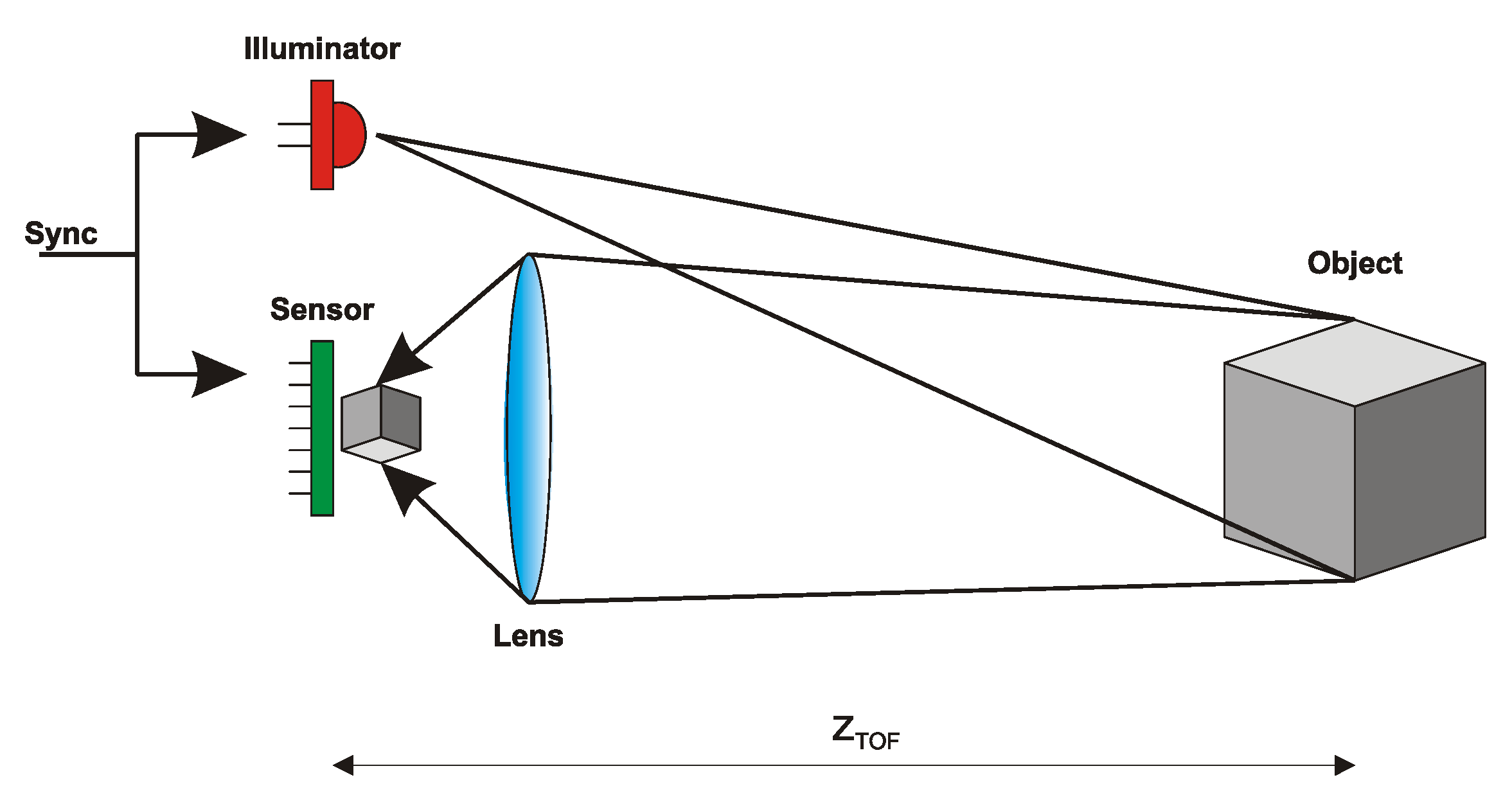
2. Model of an I-TOF Camera

All I-TOF cameras share a number of parameters and characteristics even if they are implemented using different devices. In the following, several definitions and equations will be detailed, to be used in the analysis of I-TOF performances.

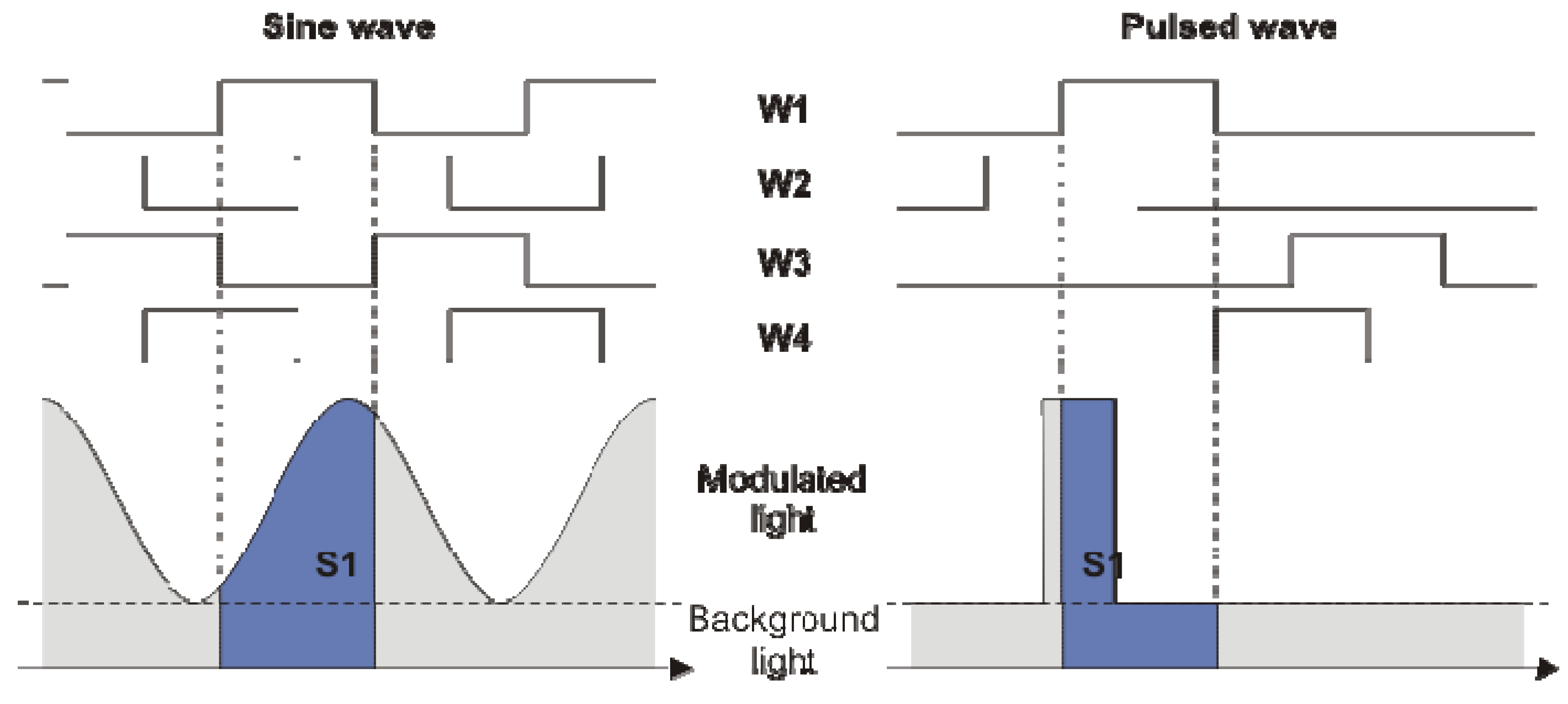
2.1. I-TOF Measurement and Power Budget

The typical setup of a time-of-flight camera is shown in Figure 1, where the measurement of the time-of-flight could be either direct or indirect.

Figure 1. Typical setup of a time-of-flight camera.

Figure 1. Typical setup of a time-of-flight camera.

The target is illuminated by a modulated source, which ideally spreads the light uniformly over the field of view. Based on the object reflectivity, a certain amount of light is diffused and collected by the camera optics, and finally focused onto the sensor area. Illuminator and sensor are properly synchronized to guarantee the relative measurement of the time needed by the light to travel two times the distance z_TOF.

As described in [2], the expression for the received power on the pixel P_pix can be obtained, assuming the object is a lambertian diffuser at a distance z:

$$P_{pix}=\frac{{\tau }_{opt}{A}_{pix}FF}{4F{\#}^2}{P}_d=\frac{{\tau }_{opt}{A}_{pix}FF\rho }{4F{\#}^2}\left(\frac{P_{src}}{{\left(2z\tan \theta /2\right)}^2}+P_{bg}\right)$$

(1)

where F# is the F-number of the optics, FF is the pixel fill-factor, A_pix is the pixel area, and τ_opt is the optics transmission efficiency. The power density P_d on the object surface is the sum of the contributions of background light and active illumination, therefore including the object reflectivity ρ. The calculation is made assuming uniform projection of illuminator power P_src on a square, with θ being the angle of emission.

When operating with low values of received power, photodetectors always operate in photocurrent integration mode: therefore, the indirect calculation of the time-of-flight must be performed on the integral of the received signal.

Figure 2. Integration windows in the case of sine wave modulation and pulsed wave.

Figure 2. Integration windows in the case of sine wave modulation and pulsed wave.

The general way of performing such a measurement consists in defining 4 integration windows, synchronized with the emitted light. A number of other methods are known for the extraction of the phase shift of the incoming signal, but the one sketched in Figure 2 is the most general one and used because of its straightforward implementation. In the case of continuous wave sinusoidal modulation the received light is integrated during 4 windows having the same frequency f_mod, with a relative phase shift of 90°. On the other hand, in the pulsed case for light pulse width of T_p, a possible method consists in having again 4 windows, two of which are needed to measure a slice of the received pulse and the whole pulse, while the other two evaluate the background contribution in similar conditions. The output signal for each of the integration windows can be written as follows:

$$V_o=\frac{q}{C_{eq}}\frac{QE({\lambda }_{src})\cdot T_{\mathrm{int}}}{hc/{\lambda }_{src}}{P}_{pix}$$

(2)

where T_int is the total integration time for each window and C_eq is the equivalent integration capacitance, which besides the effective integration capacitance includes any other gain contribution in the signal chain, that may include voltage followers, amplifiers, etc. The quantum efficiency QE is defined at the source center wavelength λ_src.

The equations that give the distance measurement are, respectively:

$$z_{TOF}=\frac{c/2}{2f_{\mathrm{mod}}}\left[1-\frac{1}{\pi }\arctan \left(\frac{V_{o3}-V_{o1}}{V_{o4}-V_{o2}}\right)\right](\text{sine})z_{TOF}=\frac{c/2}{T_p}\left(\frac{V_{o1}-V_{o3}}{V_{o2}-V_{o4}}\right)(\text{pulsed})$$

(3)

where c is the speed of light, and V_o1..o4 are the integrated signals in the windows W_1..4, respectively. To resolve the whole range, the arctangent function that takes into account also the sign of numerator and denominator must be used (the so-called “atan2”). The difference of the integrated signals guarantees that the background signal is subtracted and therefore theoretically it is not influencing the measurement, while the ratio allows the cancellation of the object reflectivity contribution. In both cases, four measurements (or two differential measurements) are needed to obtain a quantity which is independent from both the reflectivity and the background light.

2.2. Noise of Distance Measurement

Each voltage measurement V_o1..o4 is affected by a noise σ_Vo1..Vo4 which is due to both electronics noise and photon shot noise: to ease the calculations, it will be assumed that all four points have the same amount of noise σ_Vo. By applying the error propagation formula to the arctangent and to the ratio in Equation (3) of sine and pulsed modulation respectively, the following equations are obtained:

$$\begin{array}{c}{\sigma }_z=\frac{c/2}{2\pi f_{\mathrm{mod}}}\sqrt{\frac{2{\sigma }_{Vo}^2}{{\left(V_{o3}-V_{o1}\right)}^2+{\left(V_{o4}-V_{o2}\right)}^2}}(\text{sine})\\ {\sigma }_z=\frac{c/2}{T_p}\left(\frac{V_{o1}-V_{o3}}{V_{o2}-V_{o4}}\right)\sqrt{\frac{2{\sigma }_{Vo}^2}{{\left(V_{o1}-V_{o3}\right)}^2}+\frac{2{\sigma }_{Vo}^2}{{\left(V_{o2}-V_{o4}\right)}^2}}(\text{pulsed})\end{array}$$

(4)

In the sine case, the voltages are sampling the demodulated sinusoid, and the expression at the denominator in the square root is representing its amplitude: therefore, it is constant with respect to the phase shift. On the other hand, in the pulsed case the numbers involving the voltages depend from the time shift. In the following of the paper it will be useful to foresee the best distance precision; therefore the latter case can be simplified in the case of zero time delay by assuming both voltages subtractions to be equal. The expressions of the best distance precision become:

$$\begin{array}{c}{\sigma }_{z-\min }=\frac{c/2}{2\pi f_{\mathrm{mod}}}\sqrt{\frac{{\sigma }_{Vo}^2}{2V_{o\max }^2}}(\text{sine})\\ {\sigma }_{z-\min }=\frac{c/2}{T_p}\sqrt{\frac{2{\sigma }_{Vo}^2}{V_{o\max }^2}}(\text{pulsed})\end{array}$$

(5)

As it can be seen, in both cases the ratio between noise and maximum output voltage is present. Defining the equivalent modulation frequency in the case of pulsed wave as f_mod-eq = 1/(4πT_p), the best distance precision can be generally written as:

$${\sigma }_{z-\min }=\frac{c}{4\sqrt{2}\pi f_{\mathrm{mod}-eq}SN{R}_{\max }}$$

(6)

Using different techniques to extract the distance measurement, with respect to the ones illustrated in Figure 2 and Equation (3), brings to different expressions; at the same time it is possible to expect that the dependence by the SNR is similar. In this specific case, the pulsed technique seems to suffer from an intrinsic disadvantage: with similar illuminator requirements, that is f_mod = 1/(2T_p), there is a 2π decrease in the performance. This can be easily explained looking at the waveforms in Figure 2: two of the acquisitions are only for the background subtraction, without any signal, making the measurement more sensitive to noise. On the other hand, usually pulse peak power is higher and in photon-starved conditions the tradeoff may be compensated.

3. Figures of Merit

Range sensors and cameras are complex systems to compare, often relying on different techniques and devices: moreover, lack of crucial information about measurement conditions makes a fair comparison almost impossible. Indeed, camera system performances are often dependent on targeted applications.

Recently, in [13] several figures of merit were introduced: anyway, some of them tend to be misleading or of difficult evaluation. As an example, the so called “background light support” is giving the background light intensity which brings to saturation the detector, however, this number is not indicative of the effect that the background light can have on the distance measurement, which becomes problematic well before reaching the saturation of the signal.

It is our intention to introduce here some motivated figures of merit useful to understand the advantages and drawbacks of different detectors exploiting the TOF technique, of course to be paired with commonly used parameters as frame rate, pixel size, power consumption, etc. All the performances are evaluated with the sensor operating in the 3D acquisition mode, whereas a single 3D frame is composed by several acquisitions.

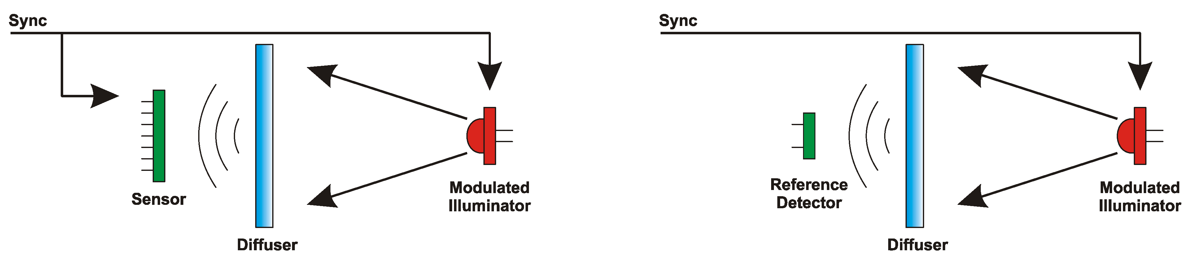
3.1. Correlated and Uncorrelated Power Responsivity

The characterization of the sensor from the electro-optical point of view can be done by illuminating through a uniform diffuser the sensitive area with a known source. The source power can be continuous, or properly modulated in intensity over time. For a given frame rate it is therefore possible to define the correlated pixel responsivity PR_corr:

the correlated power responsivity PR_corr is the transfer function from the modulated source average power density on the sensor pixel P_dpix and the output voltage V_o4 − V_o2, calculated at the maximum amplitude with respect to the phase delay.

In practical terms, the phase difference of the modulation signal between source and sensor must be optimized for maximum output voltage, while the power P_dpix should be free from any constant offset introduced by the illuminating system. A sketch of the required optical setup is shown in Figure 3. On left part the TOF sensor is characterized (V_o measurement), while on the rightmost part the light beam is characterized (P_dpix measurement), using typically a monochromatic light source of near-infrared wavelength (800–900 nm).

Figure 3. Optical setup for the evaluation of the correlated pixel responsivity: measurement of the sensor output (left) and of the incident power (right).

Figure 3. Optical setup for the evaluation of the correlated pixel responsivity: measurement of the sensor output (left) and of the incident power (right).

By using Equation (2), the ideal correlated pixel responsivity can be expressed by the following expression:

$$P{R}_{corr}=\frac{V_o}{P_{dpix}}=\frac{QE({\lambda }_{src})A_{pixel}FF}{hc/{\lambda }_{src}}\frac{q{T}_{\mathrm{int}}}{C_{eq}}\left[\frac{V}{W/m^2}\right]$$

(7)

where the integration time T_int is the part of the 3D effective frame time used to integrate the signal V_o4 − V_o2 and typically it is approximately half the total exposure, which in turn is the frame time minus the readout time. The illuminator is typically activated only when needed, but P_dpix is the average power on the pixel for the whole frame time, including all integration windows and readout time. This number is an indicator of how good is the sensor in detecting the modulated light: since in the equivalent integration capacitance C_eq also the pixel bandwidth and demodulation contrast are included, the correlated responsivity is function of the modulation frequency or pulse width. Therefore, the PR_corr parameter should be always accompanied by the frequency of the modulation signal or presented as a graph in function of the modulation frequency. For the pulsed case, the equivalent modulation frequency or the pulse width should be stated.

In the same way, the uncorrelated pixel responsivity can be defined, with a similar statement: the main difference is that the source is no more synchronized with the sensor, even if the sensor still operates with the demodulation frequency applied. Therefore:

the uncorrelated power responsivity PR_uncorr is the transfer function from a constant average power density on the sensor pixel P_bgpix and the output voltage V_o4 − V_o2.

In this case, the optical setup for the measurement is shown in Figure 4, where the modulated source has been replaced by a constant white light source: the white spectrum is chosen because, with respect to a monochromatic source, it emulates better the situation of a real environment.

Differently from the correlated responsivity case, it is not possible to extract a first order approximation of the expected PR_uncorr like in Equation (7) because the subtraction V_o4 − V_o2 makes the uncorrelated responsivity ideally zero. What determines the actual value of PR_uncorr are mismatches of the channels, imperfect background cancellation and other second-order effects: however, looking at Equation (7) all these effects can be assigned to a mismatch of C_eq between W₂ and W₄.

Figure 4. Optical setup for the evaluation of the uncorrelated pixel responsivity: measurement of the sensor output (left) and of the incident power (right).

Figure 4. Optical setup for the evaluation of the uncorrelated pixel responsivity: measurement of the sensor output (left) and of the incident power (right).

3.2. Noise-Equivalent Distance

One of the main performance indicators of 3D image sensors is the distance precision, which is the temporal noise of the distance measurement. However, to remove from this indicator all the system-related aspects, it is necessary to operate with the optical setup of Figure 3(left). In that situation, there will always be a light intensity able to bring the detector near to the saturation level: this operating condition fixes the ultimate limit of the sensor (and sensor only) distance measurement precision. To be independent from the integration time, or the frame rate, the precision has to be normalized to the square root of the bandwidth. This allows defining:

the noise equivalent distance NED is the best distance precision achievable by the sensor at the saturation limit normalized with respect to the bandwidth of the sensor.

The evaluation of the NED can be made using the setup of Figure 3(left), in conditions of maximum signal intensity, which in turn can be defined as the maximum achievable output voltage ΔV_omax minus the sigma of the non-uniformity across the array at that point FPN_ΔVomax (defined as the standard deviation with respect to the mean).

The sensor bandwidth is directly related to the 3D frame rate, and can be approximated with 1/T_frame, thus enabling a straightforward evaluation of the best performance at different frame rates. Note that T_frame is typically composed of multiple measurements, to obtain a full 3D frame.

Thanks to the expression of Equation (6) it is possible to give a theoretical evaluation of the NED of a sensor starting from some basic parameters:

$$NED=\frac{{\sigma }_{z-\min }}{\sqrt{f_{bw}}}=\frac{c\sqrt{T_{frame}}}{4\pi f_{\mathrm{mod}-eq}SN{R}_{\max }}\left[\frac{m}{\sqrt{Hz}}\right]$$

(8)

While the NED describes the best performance, often 3D image sensors operate with low incident power, far from the saturation condition. Therefore, the correlated pixel responsivity PR_corr together with the noise equivalent distance NED constitute two joint performance indicators: the first expresses the capability of the pixel in capturing and recognizing synchronized light, while the second is the effectiveness of the active circuitry in managing the signal and reducing the noise.

If showed on a xy graph, a sensor can be represented by a point (1/PR_corr, NED) where the better performances are towards the origin.

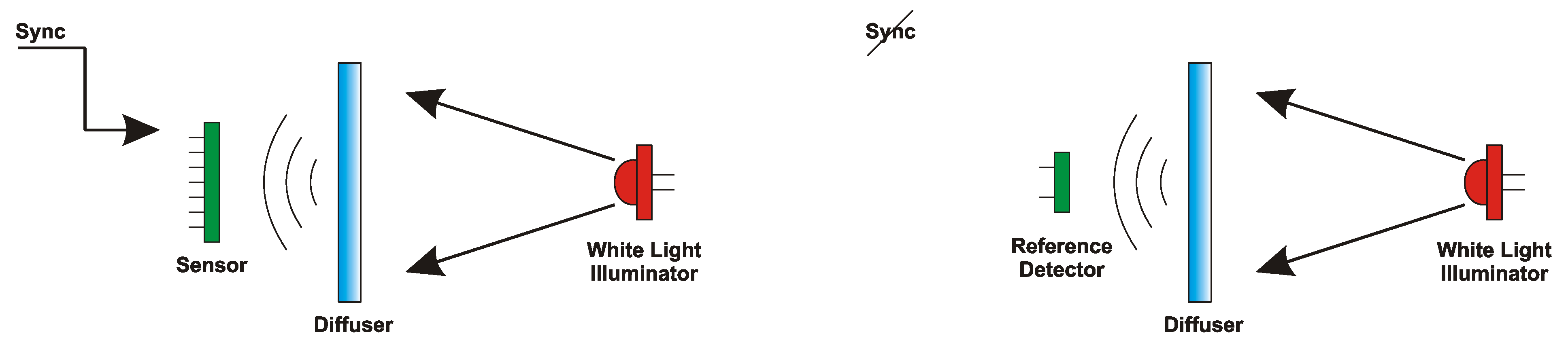
3.3. Background Light Rejection Ratio

Another important point to be evaluated for a 3D image sensor is its capability to operate in presence of background light. Obviously, the effect of the background light can be negligible when the sensor is operating with a strong echo signal, while it can have a detrimental impact when the signal is weak because of long distance or low-reflectivity object. In that sense, the figure of merit for this aspect should be independent by the imaging setup. Therefore the following can be defined:

the background light rejection ratio BLRR is the ratio between the responsivity of the sensor to background (uncorrelated) light and the responsivity to correlated light.

This parameter, usually negative if expressed in dB, gives the ability of the 3D sensor to reject background light from the signal which should carry only demodulated information and can be expressed in the following form:

$$BLRR=20\log \frac{P{R}_{uncorr}}{P{R}_{corr}}$$

(9)

The BLRR is not taking into account the method used to reject background light; therefore it is not fixing a maximum allowable background light intensity. On the other hand it can easily give the information about which is the real effect on the precision: in a sensor with a given BLRR and output SNR expressed in dB, the number BLRR + SNR represents the ratio of the illuminating power with respect to the background power in order to obtain a distance error smaller than the intrinsic distance noise (the constraint is that ΔV_uncorr < σ_ΔVcorr). Indeed, it is possible to write:

$$\frac{P{R}_{uncorr}}{P{R}_{corr}}=\frac{\mathsf{\Delta }{V}_{uncorr}{P}_{dpix}}{\mathsf{\Delta }{V}_{corr}{P}_{bg}}<\frac{{\sigma }_{\mathsf{\Delta }Vcorr}{P}_{dpix}}{\mathsf{\Delta }{V}_{corr}{P}_{bg}}=\frac{1}{SNR}\frac{P_{dpix}}{P_{bg}}$$

(10)

Equation (10) is very useful also for the system design: it allows defining the needed illuminator power, when using a sensor with a given BLRR in given background light conditions, to limit the effect with respect to the intrinsic sensor performance. In Equation (10), the ratio of illuminator and background power can be referred also to the scene and not only on the sensor plane.

4. Experimental Evaluation

Some measurements to evaluate the introduced figures of merit have been done using sensors developed in FBK, namely [2] and [13], based on pulsed and modulated techniques, respectively.

4.1. Evaluation of 3D Sensor Based on Pulsed Technique

The correlated and uncorrelated pixel responsivity has been evaluated, and in particular the correlated power responsivity has also been theoretically calculated using Equation (7). In this specific case, the value V_o4 − V_o2 can be obtained in a single frame thanks to the in-pixel correlated double sampling. Moreover, the illuminator power is pulsed and accumulated N times in a frame, with a requirement of minimum duty-cycle given by the laser specifications: therefore, the number of accumulations is the equivalent of the exposure time and determines also the 3D frame rate which can be achieved with this sensor.

Table 1. Parameters for the calculation of the figures of merit of [2].

Parameter	Value
QE	0.2
hc/λ	2.21 × 10−19 J
q	1.60 × 10−19 C
Ceq	19 fF
Apix	846.8 μm2
FF	0.34
Nacc	32…128
Tframe	18.3…35.9 ms
fmod-eq	1.59 MHz
SNRmax	170…85

Table 1. Parameters for the calculation of the figures of merit of [2].

Parameter	Value
QE	0.2
hc/λ	2.21 × 10−19 J
q	1.60 × 10−19 C
Ceq	19 fF
Apix	846.8 μm2
FF	0.34
Nacc	32…128
Tframe	18.3…35.9 ms
fmod-eq	1.59 MHz
SNRmax	170…85

Table 1 summarizes the main parameters which can be used to analytically calculate some of the presented figures of merit using Equations (7) and (8). The calculations, for the different frame rate values, give a PR_corr from 20.1 to 39.5 V/(W/m²) and a NED from 1.2 and 3.3 cm/√Hz, whereas the measurements give PR_corr from 16.7 to 31.3 V/(W/m²) and a NED from 1.4 to 3.4 cm/√Hz. While the noise equivalent distance evaluation shows a very good agreement with the calculation, the correlated power responsivity measurements result slightly smaller: this is due to the fact that the used C_eq does not include any attenuation due to finite bandwidth and charge sharing during accumulations.

Moreover, through a highly stable white light source, the uncorrelated power responsivity has been evaluated to be 0.013 V/(W/m²) for the 32 accumulations case. This gives directly a BLRR of −62 dB, which resulted to be almost constant for different number of accumulations.

4.2. Evaluation of 3D Sensor Based on Modulated Technique

Where possible, the theoretical values have been calculated in order to provide an example of the use of the introduced figures of merit. With this sensor the value V_o4 − V_o2 is obtained with two consecutive frames out of a total of four that compose the 3D image: if, for setup limitations, it is not possible to reach the maximum value of V_o4 − V_o2, it is always possible to maximize and use the demodulation amplitude:

$$\mathsf{\Delta }{V}_{o\max }=\sqrt{{\left(V_{o3}-V_{o1}\right)}^2+{\left(V_{o4}-V_{o2}\right)}^2}$$

(11)

The used prototype has a fixed readout time used also to stream the data to the PC, therefore the frame rate is not changing too much with respect to the integration time: the main parameters are shown in Table 2.

Using Equations (7) and (8) and the values of Table 2, it is possible to calculate some of the presented figures of merit. The calculations give a PR_corr from 30.2 to 31.5 V/(W/m²) and a NED from 1.5 and 1.7 cm/√Hz, whereas the measurements give PR_corr from 43.7 to 46.5 V/(W/m²) and a NED from 2.6 to 2.9 cm/√Hz. The small discrepancy between the measured and calculated value is mainly due to the approximation in the evaluation of the equivalent capacitance C_eq.

The measurements of the uncorrelated power responsivity and therefore of the BLRR gave the values of −64.4 dB for the 1ms integration time and −59.2 dB for the 2 ms integration time.

Table 2. Parameters for the calculation of the figures of merit of [13].

Parameter	Value
QE	0.2
hc/λ	3.32 × 10−19 J
q	1.60 × 10−19 C
Ceq	5 fF
Apix	100 μm2
FF	0.24
Tint	1…2 ms
Tframe	92…96 ms
fmod-eq	20 MHz
SNRmax	21…24

Table 2. Parameters for the calculation of the figures of merit of [13].

Parameter	Value
QE	0.2
hc/λ	3.32 × 10−19 J
q	1.60 × 10−19 C
Ceq	5 fF
Apix	100 μm2
FF	0.24
Tint	1…2 ms
Tframe	92…96 ms
fmod-eq	20 MHz
SNRmax	21…24

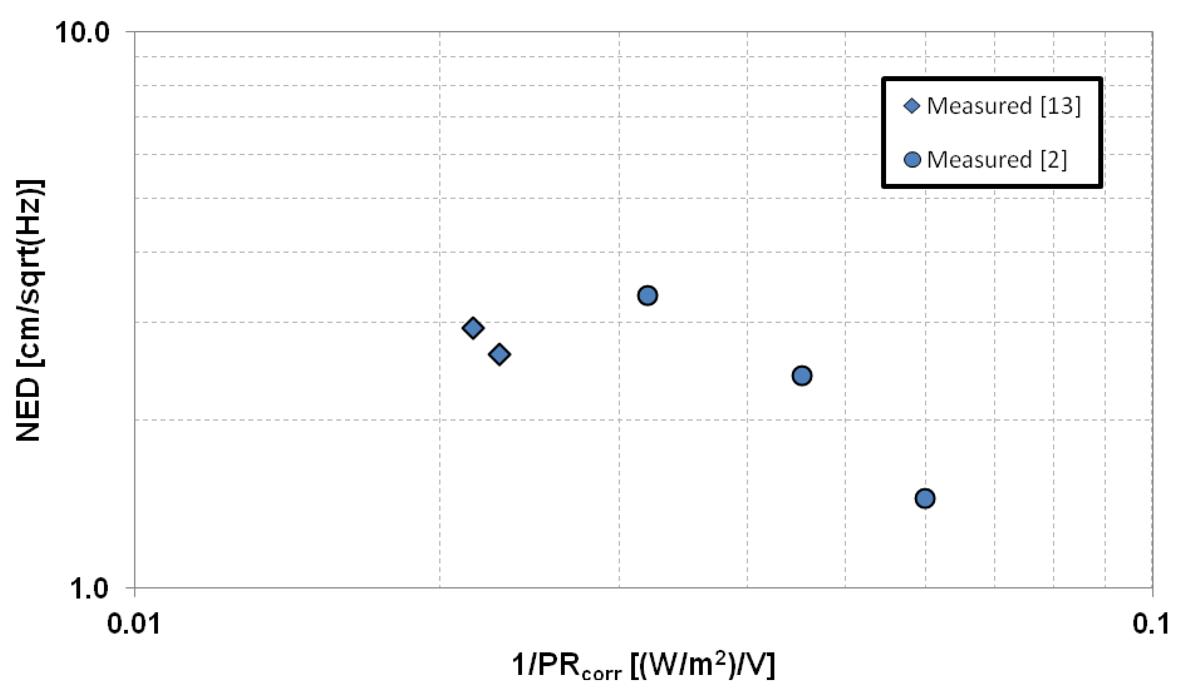
4.3. Comparison of Sensors

Besides comparing the data of Table 1 and Table 2, sensors can be easily compared by putting the NED and 1/PR_corr values on a logarithmic chart, as visible in Figure 5. For the pulsed technique, values for 32, 64, and 128 accumulations have been evaluated, while for the modulated technique, integration times of 1 ms and 2 ms have been considered.

As expected the points of individual sensors lie approximately on an iso-performance line. Despite the pulsed light sensor shows a better minimum NED for the considered integration times, it can be seen that the CW-modulated sensor shows generally better performance: indeed, the points of sensor [13] are closer to the origin. This can be explained by two considerations: one is the equivalent modulation frequency, which is lower for the pulsed light sensor, and the other is the highest sensitivity of the modulated light sensor, thanks to the very low integration capacitance value. This example demonstrates that the best distance precision should not be considered to be the sole performance indicator, as usually happens in scientific papers; this because the sensor can also have lower sensitivity and therefore it may require a much higher power to reach the same performance. The combination of NED and PR_corr gives a better and clear picture of the overall performance.

For what concerns the background light performance, the two sensors behave similarly with a BLRR in the order of −60 dB: the main difference is that the modulated light sensor has no intrinsic background light subtraction; therefore, saturation due to background light may happen for lower light levels.

Figure 5. Measured noise equivalent distance (NED) and correlated power responsivity (PR_corr) for sensors [2] and [13].

Figure 5. Measured noise equivalent distance (NED) and correlated power responsivity (PR_corr) for sensors [2] and [13].

5. Conclusions

A detailed and general analysis of the indirect time-of-flight measurement with arrays of pixels has been performed, leading to general analytical expressions of the main quantities. Exploiting these results, and experiences in the evaluation of the range imagers performances, several figures of merit have been defined, both theoretically and validated, from the measurement point of view: noise equivalent distance (NED), correlated and uncorrelated power responsivity (PR_corr and PR_uncorr), and background light rejection ratio (BLRR). As an example of the use of these figures of merit in the performance evaluation and comparison of different sensors, the results have been applied to two known cases of sensors using modulated and pulsed light: the comparison proved to be effective in evaluating pros and cons of each sensor by means of the introduced quantities.

References and Notes

1. Blais, F. Review of 20 years of range sensor development. J. Elect. Imaging 2004, 13, 231–243. [Google Scholar] [CrossRef]
2. Perenzoni, M.; Massari, N.; Stoppa, D.; Pancheri, L.; Malfatti, M.; Gonzo, L. A 160 × 120-pixels range camera with in-pixel correlated double sampling and fixed-pattern noise correction. IEEE J. Solid-State Circ. 2011, 46, 1672–1681. [Google Scholar] [CrossRef]
3. Zach, G.; Davidovic, M.; Zimmermann, H. A 16 × 16 pixel distance sensor with in-pixel circuitry that tolerates 150 klx of ambient light. IEEE J. Solid-State Circ. 2010, 45, 1345–1353. [Google Scholar] [CrossRef]
4. Spirig, T.; Seitz, P.; Vietze, O.; Heitger, F. The lock-in CCD—Two dimensional synchronous detection of light. IEEE J. Quantum Elect. 1995, 31, 1705–1708. [Google Scholar] [CrossRef]
5. Kawahito, S.; Halin, I.A.; Ushinaga, T.; Sawada, T.; Homma, M.; Maeda, Y. A CMOS time-of-flight range image sensor with gates-on-field-oxide structure. IEEE Sens. J. 2007, 7, 1578–1585. [Google Scholar] [CrossRef]
6. Van Nieuwenhove, D.; van der Tempel, W.; Grootjans, R.; Stiens, J.; Kuijk, M. Photonic demodulator with sensitivity control. IEEE Sens. J. 2007, 7, 317–318. [Google Scholar] [CrossRef]
7. Pancheri, L.; Stoppa, D.; Simoni, A. SPAD-Based Time-Gated Active Pixel for 3D Imaging Applications. In Proceedings of EOS Conference on Frontiers in Electronic Imaging, Munich, Germany, 15–17 June 2009.
8. Stoppa, D.; Massari, N.; Pancheri, L.; Malfatti, M.; Perenzoni, M.; Gonzo, L. A range image sensor based on 10-um lock-in pixels in 0.18-um CMOS imaging technology. IEEE J. Solid-State Circ. 2011, 46, 248–258. [Google Scholar] [CrossRef]
9. Mesa Imaging Website. Available online: http://www.mesa-imaging.ch (accessed on 15 November 2011).
10. PMD Technologies Website. Available online: http://www.pmdtec.com (accessed on 15 November 2011).
11. SoftKinetic Website. Available online: http://www.softkinetic.com (accessed on 15 November 2011).
12. Fotonic Website. Available online: http://www.fotonic.com/ (accessed on 15 November 2011).
13. Hafiane, M.L.; Wagner, W.; Dibi, Z.; Manck, O. Analysis and estimation of NEP and DR in CMOS TOF-3D image sensor based on MDSI. Sens. Actuat. A: Phys. 2011, 169, 66–73. [Google Scholar] [CrossRef]
14. Pancheri, L.; Stoppa, D.; Massari, N.; Malfatti, M.; Gonzo, L.; Hossain, Q.D.; Dalla Betta, G.-F. A 120 × 160 pixel CMOS range image sensor based on current assisted photonic demodulators. Proc. SPIE 2010. [Google Scholar] [CrossRef]