Remote Sensing and Modeling of Mosquito Abundance and Habitats in Coastal Virginia, USA

Abstract

The increase in mosquito populations following extreme weather events poses a major threat to humans because of mosquitoes’ ability to carry disease-causing pathogens, particularly in low-lying, poorly drained coastal plains vulnerable to tropical cyclones. In areas with reservoirs of disease, mosquito abundance information can help to identify the areas at higher risk of disease transmission. Using a Geographic Information System (GIS), mosquito abundance is predicted across the City of Chesapeake, Virginia. The mosquito abundance model uses mosquito light trap counts, a habitat suitability model, and dynamic environmental variables (temperature and precipitation) to predict the abundance of the species Culiseta melanura, as well as the combined abundance of the ephemeral species, Aedes vexans and Psorophora columbiae, for the year 2003. Remote sensing techniques were used to quantify environmental variables for a potential habitat suitability index for the mosquito species. The goal of this study was to produce an abundance model that could guide risk assessment, surveillance, and potential disease transmission. Results highlight the utility of integrating field surveillance, remote sensing for synoptic landscape habitat distributions, and dynamic environmental data for predicting mosquito vector abundance across low-lying coastal plains. Limitations of mosquito trapping and multi-source geospatial environmental data are highlighted for future spatial modeling of disease transmission risk.

1. Introduction

Vector-borne diseases such as those transmitted by mosquitoes, contribute significantly to the total disease burden in developing countries. The increase in mosquito populations following extreme weather events poses a major threat to humans due to mosquitoes’ ability to carry disease-causing pathogens. Environmental conditions such as increased rainfall and higher temperatures can lead to an increase in mosquito populations, commonly referred to as ‘blooms’. Provided there is a disease reservoir population (e.g., birds), this can lead to an increase in vector-borne disease transmission such as Eastern Equine Encephalitis (EEE) and West Nile Virus (WNV). These diseases commonly increase following extreme weather events such as hurricanes and tropical storms [1]. In order to prevent the spread of disease, it is advantageous to predict vector abundance, both spatially and temporally.

Remote sensing (RS) and Geographic Information Systems (GIS) are highly useful tools for assessing the spatial epidemiology of vector-borne diseases and analyzing human risk of infection. RS/GIS facilitate emergency planning and response for incidents ranging from natural disasters to bioterrorism, and the rapid assessment of the impact of such disasters [2]. In conjunction with traditional vector surveillance and environmental monitoring, these geospatial technologies can also help with mosquito control by predicting vector abundance. Accordingly, this study uses integrated RS/GIS to predict the abundance of the vector species, particularly Culiseta melanura as well as the combined abundance of Aedes vexans and Psorophora columbiae across Chesapeake, Virginia. Aedes vexans and Psorophora columbiae can be predicted as a combined total because these species share similar habitat preferences and population life cycles. These species share a habitat preference of ephemeral pools, such as ponding from summer season rainfall, and therefore will be referred to as the “ephemeral species” throughout this work. C. melanura is an important species because it is the primary enzootic vector of Eastern Equine Encephalitis (EEE). According to the Centers for Disease Control and Prevention (CDC), EEE is a potentially fatal virus with a 33% mortality rate (2009). C. melanura is also a potential vector of West Nile Virus (WNV). This species is found mostly in freshwater swamps, particularly subterranean crypts [3,4]. A. vexans is another important species because it is a potential epizootic vector for WNV. WNV is a potentially serious epidemic affecting humans and animals throughout North America. The virus often flares up in the summer and continues into the fall [5]. P. columbiae is also a potential vector for WNV as well as Venezuelan Equine Encepahlitis (VEE) [6]. Such knowledge of each species’ vector capacity to spread disease, habitat preferences, environmental requirements for reproduction, and life cycle are important to predictive spatial modeling.

GIS has become a pervasive technology in urban planning and environmental management, yet relatively less literature has emerged focuses on how RS and GIS can be integrated for mapping and assessing patterns of disease infection. Some studies evaluate patterns of vector or human case distributions, while others calculate risk of disease transmission based on entomological, epidemiological and environmental determinants [7]. One limitation is that these studies are often static and only predict abundance or risk at one particular time and place. This study has addressed this shortcoming by predicting mosquito abundance both spatially and temporally. In addition, many studies often use vector presence to estimate risk, rather than predicting vector abundance. According to [8], disease risk is more closely correlated with the abundance of vectors, rather than with the presence of the vector. This study has attempted to improve upon disease risk modeling techniques by predicting vector abundance rather than to simply map mosquito captures.

A given mosquito species presence is influenced by many environmental variables including temperature, precipitation, and soil moisture. Low-lying coastal plains, such as the Atlantic Coastal Plain on the USA Eastern Seaboard, are also prone to slow soil water drainage, a mosaic of interspersed human and vector habitats (swamps, ditches, and canals), and episodic impacts from tropical cyclones. Through the use of remote sensing, these habitats can be mapped and dynamic environmental variables can be measured and used to predict the habitat suitability of a particular area. To determine the suitability of areas within Chesapeake, Virginia, for mosquito habitation, a habitat suitability index (HSI) can be calculated for both groups of species for the year 2003. The HSI results along with dynamic environmental variables are incorporated into a GIS-based spatial model that calculates mosquito abundance across the study area for the summer season, June through August of 2003. Predictions were limited to this period due to the ample mosquito trap data available for these months. These months also represent the prime breeding period for these mosquitoes as the high temperatures and abundant precipitation create an ideal habitat for mosquito populations to thrive. Once abundance is predicted, the results can be used in subsequent risk models to predict the risk of disease transmission from these mosquito species.

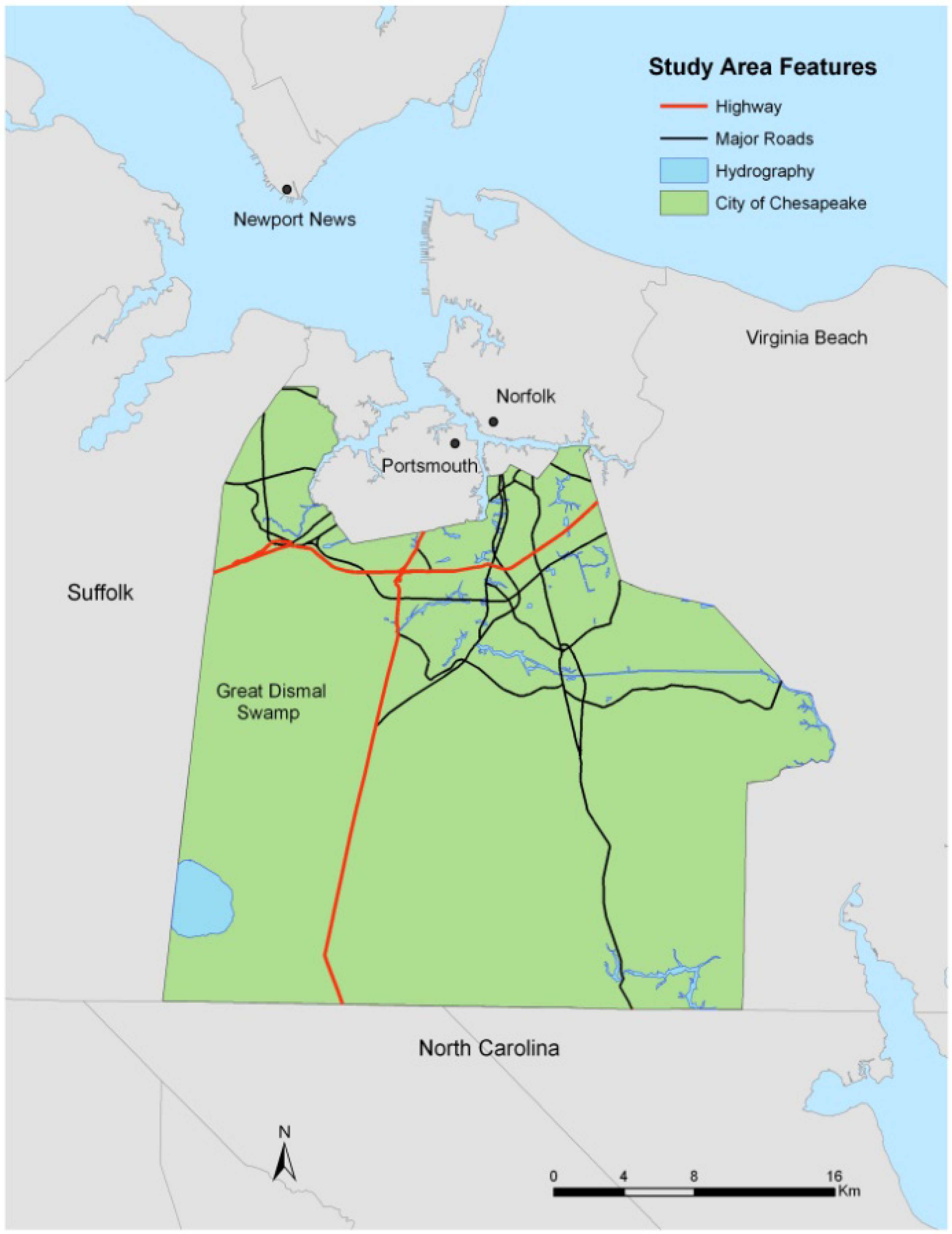
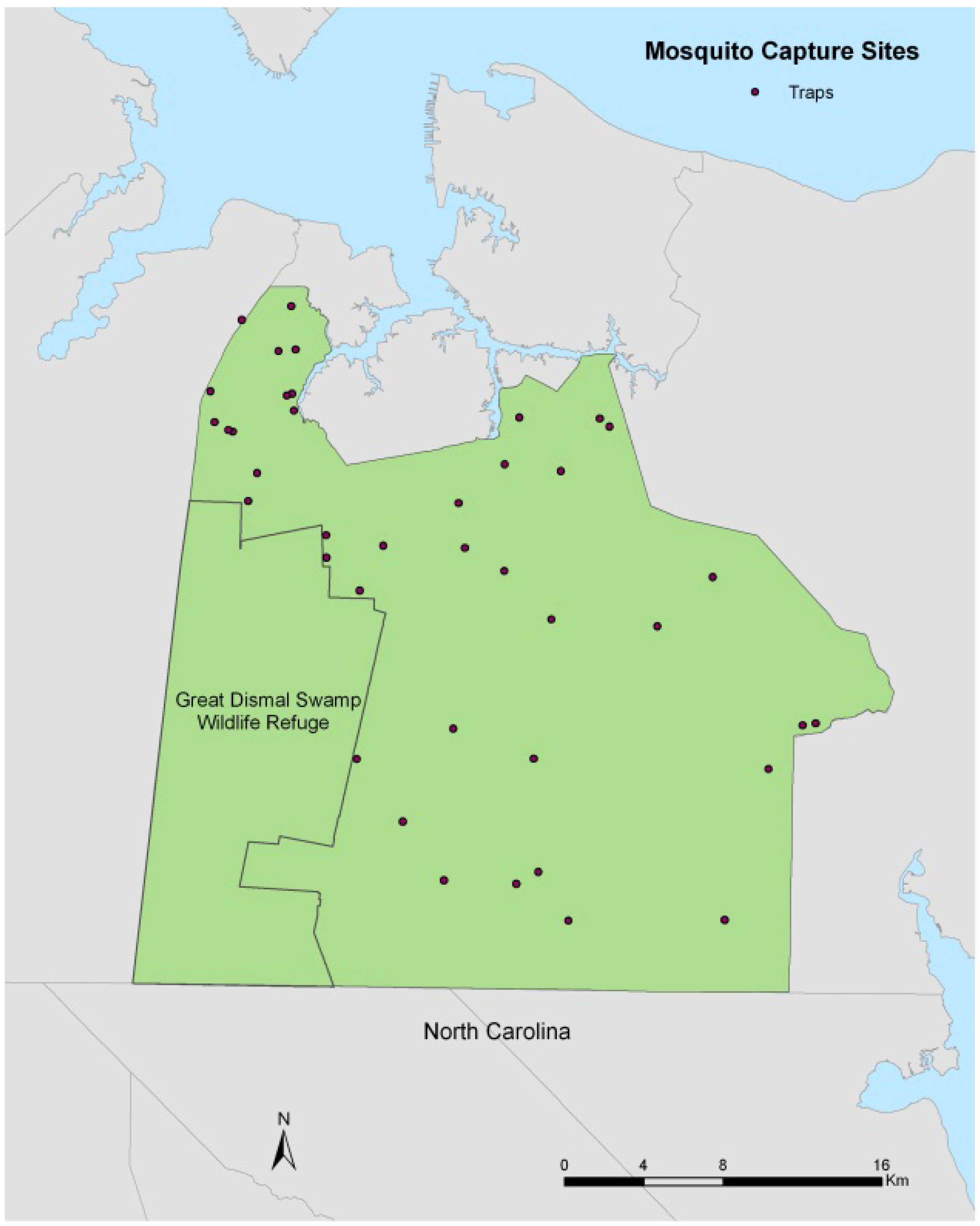
2. Study Area and Data

Chesapeake is an independent city which comprises 340 square miles (2000) of Southeastern Virginia and has a population of 220,111 (2008). The city is located in the low-lying coastal plain of Virginia and contains the northeastern portion of the Great Dismal Swamp (Figure 1). The Great Dismal Swamp serves as a large potential reservoir of avian birds and mosquitoes. Although no permanent human residents live in the swamp, large tracts of former swampland adjoin the present refuge and provide extensive cropland and suburban settlements. Much of this lowland pocosin forested wetland has been drained for agriculture and other development, resulting in extensive networks of ditches and close proximity of rural and suburban human settlements to the local drainage network and swamp alike. Because the abundance results will eventually be used to predict the risk of disease transmission to humans, it would be irrelevant to predict mosquito abundance only in the Great Dismal Swamp. Rather, the extensive wetlands and creeks within Chesapeake are quite conducive to mosquito breeding and therefore provide a suitable habitat for mosquitoes that is amenable to modeling and spatial pattern analysis.

Mosquito trap counts collected by staff in the Mosquito Control Commission were used to predict both the HSI and mosquito abundance across the study area. CO₂-baited CDC light traps were placed at over 40 locations across Chesapeake, Virginia, in 2003 (Figure 2). The year 2003 was selected owing to the greatest availability of trapping data, prior experience monitoring traps from 2001 to 2002, and the onset of subsequent spraying of larvicide and insecticides in 2004. Mosquito numbers were counted weekly at each trapping site from April through November. However, we chose to focus on the summer months, having greatest mosquito abundance June–August, which also captures potentially increased human outdoor activity and exposure. Only female captures were used in this study (male mosquitoes do not blood feed on humans.) Capture data includes the number of each species counted in the traps per week. The cumulative counts of the ephemeral species, A. vexans and P. columbiae were summed for each month as well as for the entire season. Culiseta melanura counts were also aggregated accordingly. To take into account the variation in trap nights (i.e., trapping effort), the capture data were normalized by dividing the total season’s captures by the total number of trap nights. The monthly totals were also divided by the number of monthly trap nights.

Figure 1. Study area location, City of Chesapeake, Virginia, situated on the border of the Great Dismal Swamp and the extensive estuaries of the Chesapeake Bay and its coastal tributaries.

Figure 1. Study area location, City of Chesapeake, Virginia, situated on the border of the Great Dismal Swamp and the extensive estuaries of the Chesapeake Bay and its coastal tributaries.

Figure 2. Mosquito light trap locations throughout City of Chesapeake in 2003.

Figure 2. Mosquito light trap locations throughout City of Chesapeake in 2003.

3. Methodology

3.1. Habitat Suitability Index (HSI)

In order to predict mosquito abundance, a raster spatial model was created that calculates a habitat suitability index (HSI) for both groups of mosquitoes across Chesapeake. Bellows’ modeling framework [9] for integrating habitat suitability and dynamic environmental models was applied in this study. The habitat suitability model uses mosquito trap data along with environmental variables to calculate a city-wide HSI for C. melanura and the ephemeral species, A. vexans and P. columbiae that indicates where these species are most likely to occur. For each group of species, a linear regression model was calculated which uses the season’s total mosquito counts as the dependent variables. Developing habitat suitability models for species, or affinity groups based on similar life cycles and ecotopes, improves subsequent abundance modeling by capture niche-specificity of species [10]. Assuming that mosquito presence is a function of environmental variables, select habitat attributes were used as independent variables to explain the spatial variation in mosquito capture data. Provided this methodology is feasible and valid, the approach may also be applicable to modeling human exposure and ecological interaction with vectors [11]. The habitat variables expected to best predict the spatial variation in mosquito capture data were chosen as the independent variables in the linear regression models (Table 1).

Table 1. Habitat attributes used as independent variables in habitat suitability index regression model.

Variable	Code	Data Type	Source	Description
Landsat Tasseled-cap indices, 2 July 2002	TC1-TC3	Raster: Landsat-7 ETM+	USGS	TC1 (Brightness) TC2 (Greenness) TC3 (Wetness)
Hydrologic	HYD	Vector (polygon)	NRCS	Presence of water
Percent Hydric Composition	HYDRIC	Vector (polygon)	NRCS	Soil meets requirements for hydric soil
Drain Potential	DRAIN	Vector (polygon)	NRCS	Degree of hydraulic conductivity and low water-holding capacity
Runoff Potential	RUNOF	Vector (polygon)	NRCS	Degree of potential water loss by overland flow
Water Table Depth	WTD	Vector (polygon)	NRCS	Minimum value for the range in depth to the seasonally high water table (April-June)
Available Water Storage (25 cm)	AWS25	Vector (polygon)	NRCS	Maximum value for the range of available water in plant root zones

Table 1. Habitat attributes used as independent variables in habitat suitability index regression model.

Variable	Code	Data Type	Source	Description
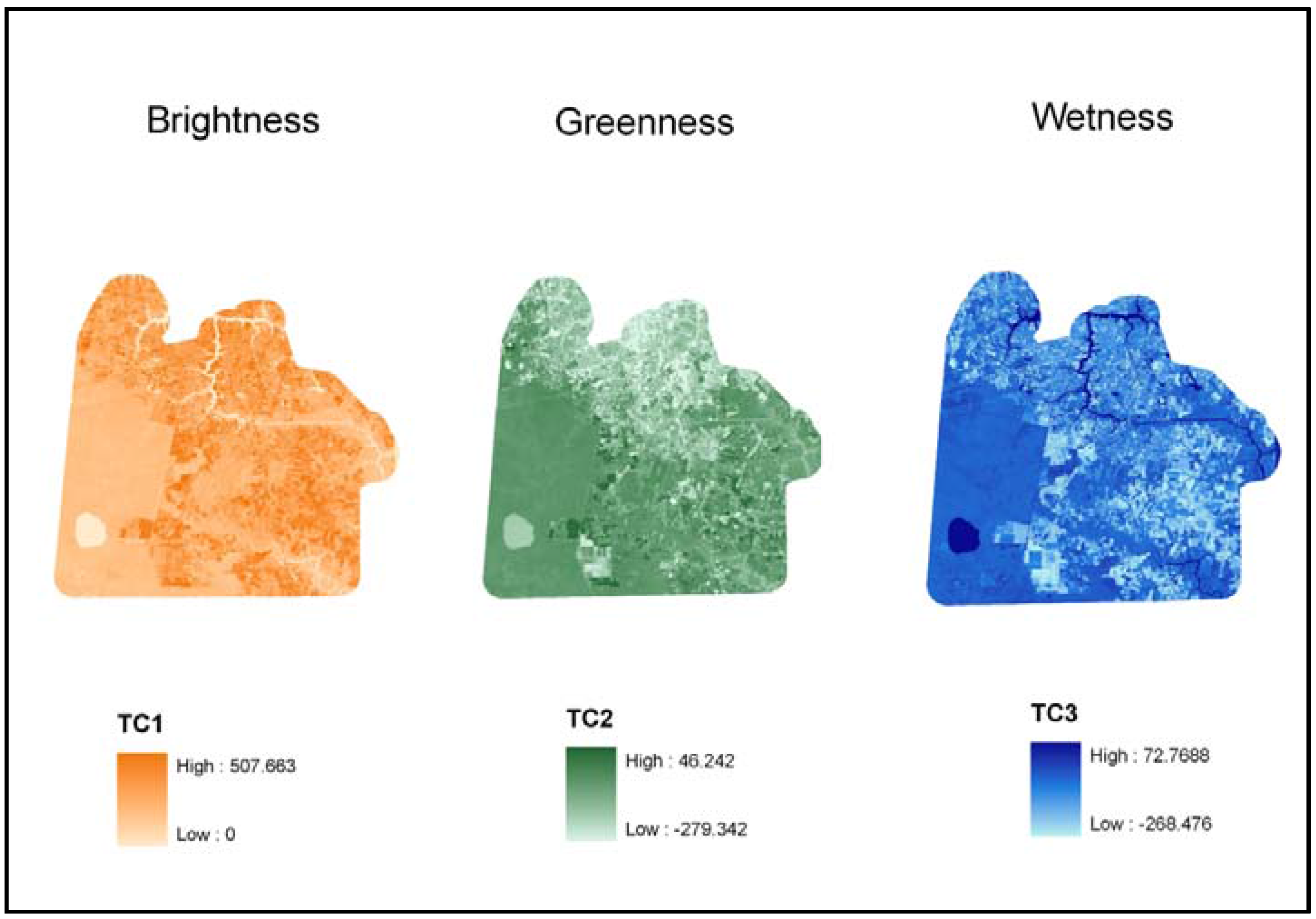
Landsat Tasseled-cap indices, 2 July 2002	TC1-TC3	Raster: Landsat-7 ETM+	USGS	TC1 (Brightness) TC2 (Greenness) TC3 (Wetness)
Hydrologic	HYD	Vector (polygon)	NRCS	Presence of water
Percent Hydric Composition	HYDRIC	Vector (polygon)	NRCS	Soil meets requirements for hydric soil
Drain Potential	DRAIN	Vector (polygon)	NRCS	Degree of hydraulic conductivity and low water-holding capacity
Runoff Potential	RUNOF	Vector (polygon)	NRCS	Degree of potential water loss by overland flow
Water Table Depth	WTD	Vector (polygon)	NRCS	Minimum value for the range in depth to the seasonally high water table (April-June)
Available Water Storage (25 cm)	AWS25	Vector (polygon)	NRCS	Maximum value for the range of available water in plant root zones

Landsat-7 Enhanced Thematic Mapper (ETM+) satellite imagery was used to produce landscape-scale evaluation of habitat suitability. A Tasseled-Cap transformation was calculated from a 5 July 2002, Landsat image acquired from the US Geologic Society (USGS). Although the year of the satellite data predates the year of mosquito data collection used in the abundance data, the study was constrained by availability of cloud-free imagery. In addition, in lieu of (unavailable) cloud-free high-resolution imagery, this July 2002 image data serves as a landscape characterization, or proxy, and emphasizes the typicality of summer season imagery for the region and the application of the satellite data to capture synoptic, landscape-scale spatial and spectral habitat variation. Furthermore, the Tasseled-Cap transformation of Landsat multispectral data is used to separate brightness, greenness, and wetness bands within satellite imagery [12]. Brightness, greenness, and wetness indices are useful for characterizing such biophysical spatial patterns associated with mosquito habitat suitability and were chosen over land cover classification in order to characterize these environmental gradients. Brightness (Tasseled Cap layer 1, TC1) is a measure of reflectance and is correlated to the texture and moisture content of soils [13]. Greenness (TC2) is a measure of the density of green vegetation present, while wetness (TC3) is a measure of the moisture in soils, vegetation, and other surface cover [14,15]. The transformed values are reprojected onto three orthogonal axes (TC1-TC3) which were used as the independent variables in the linear regression equations (Figure 3). Selected soil attributes (Table 1) were chosen as the explanatory variables in the habitat suitability model. The variables were selected based on their relationship to mosquito habitat preferences, particularly soil moisture. According to Tanser, Sharp, and le Sueur [16], soil moisture is an important factor in mosquito survival. Soil survey data was acquired from the US Department of Agriculture (USDA) National Resources Conservation Service’s (NRCS) soil data mart. Chesapeake soil data for 2002 was exported into SSURGO format (Soil Survey Geographic Data) and then converted into grid format. The grid values were reclassified into standard numeric values used by SSURGO. Since the effect of variables influencing landscape and ecosystem-level patterns, processes, and functions is scale-dependent [17], the environmental variables were analyzed for scale dependent correlations with abundance. For each habitat attribute, the spatial scale (grid resolution) that was most strongly correlated with mosquito captures for each species group was retained for the HIS model predictors. ArcGIS Spatial Analyst tools were used to rescale the raster values for each attribute with the focal neighborhood mean of the pixels with the corresponding spatial scale.

Figure 3. Derived Landsat-7 ETM+ Tasseled-cap indices for study area, brightness (TC1), greenness (TC2), and wetness (TC3).

Figure 3. Derived Landsat-7 ETM+ Tasseled-cap indices for study area, brightness (TC1), greenness (TC2), and wetness (TC3).

Because the predictor variable data is time invariant across the year, a single HSI was calculated for each mosquito group to represent the entire breeding season. Linear regression models were used to quantify the HSI for each species group. The habitat attributes (X) are weighted using the corresponding regression coefficient (b) and incorporated into a regression equation to calculate habitat suitability (Equation (1)). The final HSI’s were created on the basis of a 30 m pixel grid, which serves as the unit of observation.

HSI = a + b₁(X₁) + b₂(X₂) … b_p(X_p)

(1)

Using the statistical software PASW Statistics 17.0, linear regression models were calculated for each species group to predict the effect of the independent variables on mosquito counts. For each group of species, the total normalized mosquito count for June through August was regressed upon the corresponding independent variable grid values. Because there are 40 traps and the study period covers three months, ideally the sample size (n) should have been 120 traps. However, not every trap was counted each month, reducing the sample size to 93 traps. Tests for multicolinearity were analyzed using the computed variance inflation factors (VIF), such that variables with collinear relationships were not duplicated in the models if above a threshold (VIF < 5 to retain.) Once the regression models were calculated (Equations (2) and (3)), the regression equations could be encoded into the spatial model using ArcGIS modelbuilder to generate a habitat suitability index for each species group.

HSI_Ep = [−111.719 + 20.7 (RUNOFF) − 0.283 (WTD) + 0.517 (TC2) + 20.807 (HYD) − 7.925 (DRAIN)]

(2)

HSI_Cm = [−532.162 + 510.400 (RUNOF) + 51.574 (AWS25) − 5.357 (TC2) + 0.193 (TC3) + 11.926 (DRAIN)]

(3)

where HSI_Cm = the habitat suitability index for Culiseta melanura and HSI_Ep = the habitat suitability index for the ephemeral species.

3.2. Mosquito Abundance Model

The habitat suitability indices could be used in accordance with other environmental variables to build a model that predicts mosquito abundance both spatially and temporally. Using ArcGIS Model Builder, an equation was constructed for both groups of mosquitoes to predict mosquito abundance for each month from June to August of 2003. Linear regression models were used to quantify the effect of certain climate variables on mosquito trap counts for each month. The model incorporates environmental variables that are known to influence mosquito presence. Topographic soil moisture index (TMI), monthly precipitation, average weekly air temperature (AWAT), and the interactive effects of temperature and precipitation were used as the independent variables in the models. The regression equations were then used to calculate monthly indices to represent the weighted effects of the variables on mosquito captures for both mosquito groups. The indices representing the weighted effects of the environmental variables on abundance were abbreviated as “EEV”. The EEV monthly indices for both groups of species were each overlaid with the corresponding HSI grid to calculate the monthly mosquito abundance.

The predictor variables used in the linear regression models were chosen based on their influence on mosquito presence. Because mosquitoes prefer soils with a high moisture content, a topographic soil moisture index (TMI) was used as a variable to explain the variation in mosquito presence. TMI is a derivative of slope and flow accumulation (Equation (4)). The TMI grid was calculated using an equation derived from Beven [18] which is shown below.

TMI = ln (A/tan β)

(4)

where A = flow accumulation surface and β = slope surface. Raster map algebra was used to calculate this equation on a per pixel basis to create a 30 m TMI grid.

Because mosquito life cycles are affected by temperature, the average weekly air temperature (AWAT) was also used as an explanatory variable in the linear regression models (Equation (5)). Spatially dependent temperature grids for Chesapeake, Virginia, are not available for 2003. AWAT constant-value grids are available from the National Climatic Data Center (NCDC), collected at the NWS Station at Chesapeake Regional Airport (KCPK). Each grid displays the mean weekly temperature in Fahrenheit degrees across Chesapeake. For each month, the weekly average temperatures were averaged and attributed to the grid. The temperature values were normalized and rescaled using the following equation:

$$X_r=\frac{X_O - X_{min}}{X_{max} - X_{min}} \times 100$$

(5)

where X_r = the normalized and rescaled monthly temperature value (0–100), X_O = the observed temperature value, X_min = the minimum monthly temperature value, and X_max = the maximum monthly temperature value.

Precipitation affects mosquito habitats and breeding patterns, therefore, rainfall was used as an independent variable to explain the variation in mosquito trap data. Monthly precipitation grids were obtained from the PRISM Climate Group. The precipitation data sets are created using the Parameter-elevation Regressions on Independent Slopes Model (PRISM) climate mapping system [19]. Chesapeake experienced a particularly wet summer in 2003 due to Hurricane Isabel, which made landfall in North Carolina on 18 September 2003 [20]. PRISM grids display the nationwide average rainfall in millimeters for each month of the study period. Grids were downloaded in ASCII format and converted to raster format. Each monthly grid was clipped to the full extent of the study area and the values were normalized and rescaled from 1 to 100 using the following Equation (6):

X_r = (X_O/X_max) × 100

(6)

where X_r = the normalized and rescaled monthly temperature value (0–100), X_O = the observed value, and X_max = the maximum value.

To account for possible interaction between temperature and precipitation, the product of temperature and precipitation was used as an independent variable in the models. The corresponding monthly precipitation and temperature grids were multiplied to generate monthly grids that display the interactive effects of the two variables.

Spatial Analyst tools were used to extract the independent variable data for each coinciding trap point into a database. The resulting table could then be used in the software program PASW Statistics 17.0 to create a linear regression model for both species groups that use the independent variables to explain the variation in monthly mosquito trap data. In order to normalize the mosquito capture data, the mosquito counts were log transformed to calculate the natural log of the values. A model was created for each species in which the log transformed capture value at each trap site was regressed upon the corresponding monthly independent variables. Once the linear regression equations were calculated for both species groups, the equations could be used to calculate the monthly EEV. The regression coefficients from each equation were used to calculate the weighted influence of the independent variables on the mosquito trap counts. The equations were calculated using raster map algebra on a per-pixel basis and incorporated into each abundance model. Equations (7) and (8) for the linear regression models are shown below:

EEV_Ep = −0.015 (Temperature × Precipitation) + 1.462 (Temperature) + 1.193 (Precipitation) + 0.000 (TMI)

(7)

EEV_Cm = −0.020 (Temperature × Precipitation) + 1.881 (Temperature) + 1.444 (Precipitation) + 0.016 (TMI)

(8)

where EEV_Ep = the effects of the environmental variables on ephemeral species abundance for a particular month, and EEV_Cm = the effects of the environmental variables on C. melanura for a particular month. The results were each represented as a 30 m grid. Within each model, the monthly EEV grids were used along with the HSI grids to predict abundance. Abundance was predicted for each month on a pixel-by-pixel basis using Equations (9) and (10):

Abundance_Cm = HSI_Cm × EEV_Cm

(9)

Abundance_Ep = HSI_E × EEV_E

(10)

where Abundance_Cm = total C. melanura abundance for a particular month and Abundance_Ep = total ephemeral species abundance for a particular month. For each month, the abundance values were rescaled to reflect the season’s overall abundance using the equation:

$${\text{Abundance}}_r=\frac{{\text{Abundance}}_O - {\text{Abundance}}_{min}}{{\text{Abundance}}_{max} - {\text{Abundance}}_{min}}$$

(11)

where Abundance_r = the rescaled abundance for a particular month, Abundance_O = the observed abundance for the month, Abundance_min = the minimum abundance for the month, and Abundance_max = the maximum abundance for all months within the study period.

4. Results and Discussion

4.1. Habitat Suitability Index (HSI)

The habitat suitability maps for both groups of mosquitoes are each unique and representative of the corresponding mosquito preferences (Figure 4). The R² value for the HSI regression model (Table 2) indicates that independent variables explain 35.6% of the variation in ephemeral species trap data. With a regression coefficient of 1.065 (Table 3), TC1 brightness is the most significant variable for predicting the suitable habitat for ephemeral species. The correlation between brightness and habitat suitability is not particularly strong. However, because high brightness values represent a lack of vegetation, this weaker correlation between HSI and TC1 is to be expected. The preferred habitat of A. vexans and P. columbiae is ephemeral pools which do not correspond with regions of high brightness. A few of the highly suitable regions do in fact overlay with bright regions. These regions may represent suburban areas where mosquitoes may be breeding in containers. According to the regression model, TC2 or greenness is another important variable in predicting habitat suitability. The model indicates that greenness is positively correlated with habitat suitability. Like the brightness variable, the regression coefficient for the greenness variable is modest. This coefficient of 0.517 would explain the lack of correlation between HSI and TC2. Overall, the most suitable habitat for A vexans and P. columbiae appear to be regions covered in proximity to high moisture, including open water such as rivers and lakes. The unsuitable regions do not appear to have a strong correlation with any particular type of land cover.

The habitat suitability index for C. melanura differs considerably from the ephemeral species model. The R² value (Table 2) indicates that independent variables explain 33.9% of the variation in C. melanura trap data. With a significance value of 0.004 (Table 3), the soil runoff variable proved to be the most significant attribute in the habitat suitability model for C. melanura. According to the linear regression model, runoff and suitability are positively correlated. Because higher runoff values actually represent potential accumulated runoff and resulting moisture, it is expected that highly suitable areas should overlay with high runoff values. The habitat suitability map affirms the significance of the runoff variable. By overlaying the runoff variable onto the habitat suitability map, it is clear that the regions with the highest suitability appear to have either soils with low runoff potential or are covered by water. Available soil water holding capacity is another significant variable in predicting habitat suitability for C. melanura. The linear regression results indicate that soil water holding capacity and habitat suitability are positively correlated. An overlay of the two variables confirms that as water holding capacity increases, so does habitat suitability. Because C. melanura prefer a moist habitat, it makes sense that a lack of runoff and increase in available water holding capacity are associated with an increase in habitat suitability. In general, the most suitable areas for C. melanura habitation appear to be swamps and marshes. This observation is expected since swamps are the preferred habitat for these species. Unlike the ephemeral species, open water areas such as rivers were predicted to be very unsuitable for C. melanura.

Figure 4. Habitat Suitability Index (HSI) for ephemeral species group and C. melanura. The HSI values were calculated using Equations (2) and (3). Values were classified into 5 equal interval classes.

Figure 4. Habitat Suitability Index (HSI) for ephemeral species group and C. melanura. The HSI values were calculated using Equations (2) and (3). Values were classified into 5 equal interval classes.

Table 2. Summary of the HSI linear regression models.

Species	R2	Adjusted R2	F	Sig.
Ephemeral	0.356	0.238	3.035	0.018
C. melanura	0.339	0.236	3.287	0.017

Table 2. Summary of the HSI linear regression models.

Species	R2	Adjusted R2	F	Sig.
Ephemeral	0.356	0.238	3.035	0.018
C. melanura	0.339	0.236	3.287	0.017

Table 3. Results of the HSI linear regression models.

Species	Variable	B	t	Sig.
Ephemeral	Constant	−111.719	−1.629	0.113
Ephemeral	TC1	1.065	3.106	0.004
Ephemeral	TC2	0.517	1.805	0.080
Ephemeral	HYD	20.807	0.762	0.452
Ephemeral	DRAIN	−7.925	−1.212	0.234
Ephemeral	RUNOFF	20.730	0.904	0.373
Ephemeral	WTD	−0.283	−1.266	0.215
C. melanura	Constant	−532.162	−2.818	0.008
C. melanura	TC2	−5.357	−2.599	0.014
C. melanura	TC3	0.193	0.059	0.953
C. melanura	DRAIN	11.926	0.531	0.599
C. melanura	RUNOFF	510.400	3.096	0.004
C. melanura	AWS25	51.574	1.924	0.063

Table 3. Results of the HSI linear regression models.

Species	Variable	B	t	Sig.
Ephemeral	Constant	−111.719	−1.629	0.113
Ephemeral	TC1	1.065	3.106	0.004
Ephemeral	TC2	0.517	1.805	0.080
Ephemeral	HYD	20.807	0.762	0.452
Ephemeral	DRAIN	−7.925	−1.212	0.234
Ephemeral	RUNOFF	20.730	0.904	0.373
Ephemeral	WTD	−0.283	−1.266	0.215
C. melanura	Constant	−532.162	−2.818	0.008
C. melanura	TC2	−5.357	−2.599	0.014
C. melanura	TC3	0.193	0.059	0.953
C. melanura	DRAIN	11.926	0.531	0.599
C. melanura	RUNOFF	510.400	3.096	0.004
C. melanura	AWS25	51.574	1.924	0.063

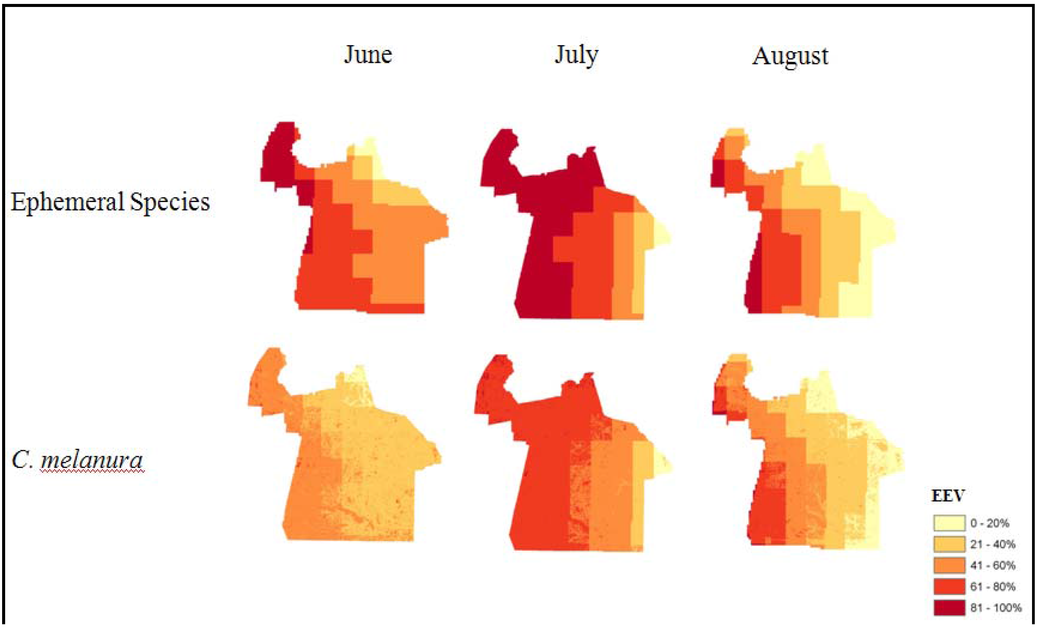
4.2. Effects of the Environmental Variables (EEV)

The results of the EEV linear regression models (Table 4) reveal the relationship between the environmental variables and mosquito trap data. For the ephemeral species, the model indicates that the independent variables explain 27.0% of the variation in ephemeral species counts. Temperature, precipitation, and the combined effects of temperature and precipitation are all significant variables in the ephemeral species and C. melanura abundance model (Table 5). However, the regression results indicate that the TMI variable is not a significant variable in predicting ephemeral species or C. melanura abundance. Temperature and precipitation are both positively correlated with mosquito abundance. This was expected since an increase in these conditions often produces habitats conducive to mosquito breeding. Based on its low regression coefficient, it can be concluded that the combined effects of temperature and precipitation did not have a strong influence on ephemeral species or C. melanura abundance.

Table 4. Summary results of the EEV linear regression models.

Species	R2	Adjusted R2	F	Significance
Ephemeral	0.270	0.235	7.846	0.000
C. melanura	0.405	0.377	14.793	0.000

Table 4. Summary results of the EEV linear regression models.

Species	R2	Adjusted R2	F	Significance
Ephemeral	0.270	0.235	7.846	0.000
C. melanura	0.405	0.377	14.793	0.000

Table 5. Results of the EEV linear regression model.

Species	Variable	B	t	Significance
Ephemeral	Constant	−104.888	−2.875	0.005
Ephemeral	Precipitation	1.193	2.989	0.004
Ephemeral	Temperature	1.462	2.987	0.004
Ephemeral	Precip_Temp	−0.015	−3.108	0.003
Ephemeral	TMI	0.000	−0.006	0.995
C. melanura	Constant	−138.191	−3.298	0.001
C. melanura	Precipitation	1.444	3.295	0.001
C. melanura	Temperature	1.881	3.508	0.001
C. melanura	Precip_Temp	−0.020	−3.498	0.001
C. melanura	TMI	0.016	1.224	0.224

Table 5. Results of the EEV linear regression model.

Species	Variable	B	t	Significance
Ephemeral	Constant	−104.888	−2.875	0.005
Ephemeral	Precipitation	1.193	2.989	0.004
Ephemeral	Temperature	1.462	2.987	0.004
Ephemeral	Precip_Temp	−0.015	−3.108	0.003
Ephemeral	TMI	0.000	−0.006	0.995
C. melanura	Constant	−138.191	−3.298	0.001
C. melanura	Precipitation	1.444	3.295	0.001
C. melanura	Temperature	1.881	3.508	0.001
C. melanura	Precip_Temp	−0.020	−3.498	0.001
C. melanura	TMI	0.016	1.224	0.224

The monthly EEV grids (Figure 5) illustrate the weighted impacts of the environmental variables on mosquito counts. The EEV values were scaled from 0 to 100 to represent the percent influence of the variables on mosquito captures. The EEV results are very similar for both groups of mosquito species. From June through August, WSC values increase moving from east to west. The effect of the independent variables on mosquito counts is particularly high in western Chesapeake across all months. In July, the EEV values are especially high across Chesapeake. The environmental variables were predicted to have more than an 81% influence on mosquito numbers across a large portion of the city. Compared to the EEV values for the ephemeral species, the EEV values for C. melanura are relatively lower. There are very few regions where the independent variables have more than an 80% influence on C. melanura captures.

Figure 5. The effects of the environmental variables on mosquito abundance. Values were separated into five equal interval classes that represent the percent effect on abundance.

Figure 5. The effects of the environmental variables on mosquito abundance. Values were separated into five equal interval classes that represent the percent effect on abundance.

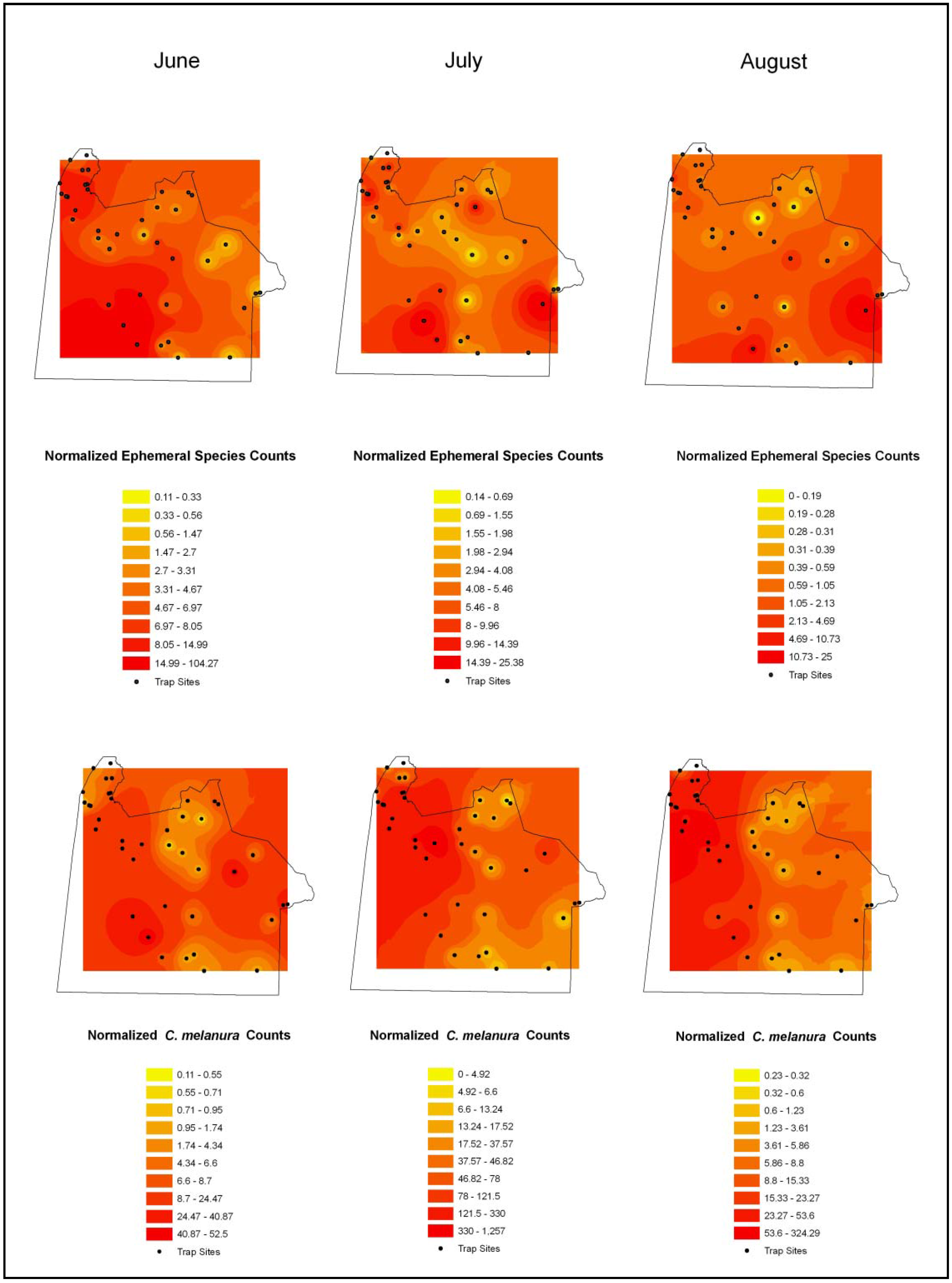
4.3. Mosquito Abundance

The mosquito abundance results (Figure 6) appear to be representative of each species’ breeding and habitat preferences. The rescaled abundance values for both groups of mosquitoes were classified into quantiles to represent different levels of abundance and were rendered on the same scale across all months. Although there is significant variation in abundance between the mosquito groups, similar spatial and temporal patterns can be seen with both groups.

The abundance model results for the ephemeral group strongly reflects the HSI results (Figure 4). As the HSI model suggests, ephemeral species abundance is very high in rivers and open water regions from June through August. In general, abundance values are highly reflective of the EEV grids (Figure 5). Like the EEV values, monthly abundance appears to increase going from east to west across Chesapeake. The abundance results for C. melanura) also show patterns consistent with the HSI results. The HSI model predicted that open water areas such as rivers would be unsuitable for C. melanura. Accordingly, the abundance model predicted that there would be a very small number of these species in open water areas. Based on the HSI results, the model predicted a high abundance of C. melanura in wetlands. The predicted high abundance of this species in wetlands is no surprise since swamps are the preferred habitat of this species.

Based on the EEV indices, we can conclude that temperature, rainfall, and TMI had the greatest impact on mosquito presence in western Chesapeake. Consequently, populations of A. vexans, P. columbiae, and C. melanura were predicted to be very high in western Chesapeake. This western region where abundance is especially high, surrounds the Great Dismal Swamp. It is no surprise that abundance is predicted to be high in this region, as the Great Dismal Swamp is known to be heavily populated with mosquitoes [21]. The wet conditions of the swamp provide an ideal habitat for mosquitoes to breed. These high abundance regions in the west are mostly covered by wetlands or cultivated croplands. Swamps and wetlands are known to be the prime breeding grounds for C. melanura. Cultivated croplands also have been proven to be ideal habitats for mosquitoes. According to [22], agricultural runoff and irrigation from cultivated croplands can support mosquito presence. Ditches and temporary pools of water can also serve as breeding grounds for mosquitoes. In regard to the ephemeral species, the high numbers predicted to reside in rivers and open water was expected. According to Crans [4], the largest numbers of these species are found in flood plains where rivers overflow their banks, but significant numbers can be produced from virtually any area where fresh ground water accumulates on an intermittent basis.

Figure 6. Monthly abundance of the ephemeral species for each month with values classified into quantiles.

Figure 6. Monthly abundance of the ephemeral species for each month with values classified into quantiles.

Comparatively, eastern Chesapeake is predicted to have a low monthly abundance of both types of mosquitoes. These predictions are partially based on the linear regression model which predicted that the environmental variables would have a limiting effect on mosquito presence in central and eastern Chesapeake. This prediction may be partly attributed to the limited number of mosquito captures in eastern Chesapeake. In general, the traps on the eastern side of the city had significantly fewer mosquitoes than the western city (adjoining the Great Dismal Swamp.) Eastern Chesapeake is covered by various types of land cover but overall less area and density of stream and forested wetlands. Agricultural land such as cultivated croplands and pastures cover much of southeastern Chesapeake. Although irrigation and runoff from cultivated land can support mosquito populations, these regions are expected to be a poorer habitat for mosquitoes due to the high drainage potential. One pattern among the abundance results can be seen in northern Chesapeake, particularly on the northern tip of the city. This region was predicted to have a very low abundance of both mosquito types in July and August. The northern portion of Chesapeake is dominated by low and high intensity developed land. Because urban areas are not the primary habitat of the three mosquito species under consideration, these developed areas are not expected to have a large number of mosquitoes. Another obvious trend is the low number of mosquitoes predicted for August. The trap data indicates that August had significantly less mosquito captures in August compared to the other months. The capture data is surprising since Hurricane Isabel struck Chesapeake in September of 2003. The average temperature across Chesapeake was higher in August compared to other months, which would potentially increase the number of mosquitoes.

To determine the predictive nature of the trap data and evaluate the accuracy of the model, the results of the abundance model can be compared to the surfaces interpolated from the trap data. Using the Inverse Distance Weighting (IDW) method, a surface was interpolated for the monthly normalized mosquito trap counts (Figure 7). One similarity between the interpolated surfaces and the model results is the concentration of high abundance regions in western Chesapeake. Like the abundance results, western Chesapeake was interpolated to have a high abundance of C. melanura for all three months. Ephemeral species abundance was also very high across western Chesapeake in June, while trap counts were moderately high in July and August. Overall, the interpolated surfaces show more spatial and temporal variation compared to the model results. The interpolated surfaces show that mosquito abundance varies across the city rather than increasing continuously from east to west. However, using the interpolation method to estimate the distribution of mosquito counts can be limiting. For example, in eastern Chesapeake, ephemeral species abundance was interpolated to be high in July and August, yet based primarily on only one trap site. The high abundance of this particular trap caused a large portion of eastern Chesapeake to have a high abundance of ephemeral species. If the trap data set included more trap sites, the IDW approach could more accurately interpolate the number of mosquitoes across Chesapeake. Another limitation is that many of the trap sites were not counted during certain months. If the trap data included a more even distribution of trap sites and regular count intervals, these surfaces could be a more reliable source for estimating mosquito abundance. The abundance model on the other hand, may be more accurate due to the various determinant variables taken into account and less reliance up on any one point for spatial interpolation.

Figure 7. Interpolated surfaces of the normalized monthly trap counts for the ephemeral species symbolized using a quantile classification.

Figure 7. Interpolated surfaces of the normalized monthly trap counts for the ephemeral species symbolized using a quantile classification.

5. Conclusions

As vector-borne diseases continue to persist and emerge, many researchers and public health officials are concerned with estimating and mapping disease risk, particularly in low-lying coastal zones prone to tropical cyclones. This study has approached and demonstrated risk estimation including relatively static factors (land cover) and dynamic variables (meteorology) for predictive modeling. These models identified potential habitat and predicted mosquito abundance, key factors in the risk of disease transmission. Using only vector presence to estimate risk can be constraining because mosquitoes are influenced by many interacting factors, particularly climatic variables [23]. By incorporating dynamic environmental variables into the mosquito abundance model, the abundance results may be more accurate than relying on vector counts and spatial interpolation alone. A next logical step is a focus on human activity space and relative vulnerability and reservoir populations for the pathogens.

Although this study has attempted to avoid the pitfalls commonly involved with predicting the risk of disease transmission, this study has revealed limitations. One limitation of the abundance model was the uneven distribution of trap sites across the city. Southeastern Chesapeake, in particular, has a limited number of mosquito traps compared to the rest of the city. With a broader range of trap locations, the linear regression model may have more accurately predicted the effects that the environmental variables had on mosquito presence. Another issue with the trap data is the inconsistency in the frequency of trap counts. In other words, trap captures were counted on approximately bi-weekly intervals. Although the trap counts were normalized to take into account the varying number of trap nights (trapping effort), uniform trap counts could potentially have led to more sensitive model results. Some of the environmental variables may have also been limiting to the mosquito abundance model. The temperature dataset, for instance, may have been only modestly helpful to the model because the monthly temperature values were so gradual and slightly variable across the study area. If the temperature values had been more strongly spatially-dependent, the relationship between temperature and the trap data may have been more significant. Other spatially-dependent variables may have been considered for this study. Wind speed or prevailing direction may also have been useful variables for estimating vector abundance. Wind can interact with the flight activity of mosquitoes and help disperse them to new areas [24] and so could provide insights in future research.

The models created in this study could be applied to another city to identify the mosquito vector-borne disease hazard. By predicting areas of high vector abundance, the mosquito abundance model can potentially help officials target where to implement mosquito control efforts. This could reduce the high cost associated with mosquito control practices such as insecticide use. This allows for increased interruption of the disease transmission as well as the saving of resources, personnel and control products, by directing their efficient application and utilizing advances in available remotely sensed high resolution and LiDAR data [25]. The ultimate goal of this study was to incorporate the abundance results for deriving models along with human vulnerability data to quantify the risk of disease transmission from mosquitoes. By identifying high-risk areas in advance, environmental and public health officials can improve the efficacy of disease prevention measures and also minimize pesticide usage by integrated management using satellite data such as Landsat [26]. Specifically, public health and emergency managers can target where to implement surveillance, early-warning systems, abatement, and educational programs. Knowing where infectious diseases are likely to emerge could also aid health workers in diagnosing and treating patients promptly. Our results encourage further studies to employ techniques such as those developed to prevent the occurrence and spread of infectious diseases.

References

1. Toole, M.J. Communicable diseases and disease control. In The Public Health Consequences of Disasters; Noji, E.K., Ed.; Oxford University Press: New York, NY, USA, 1997; p. 81. [Google Scholar]
2. Waring, S.; Zakos-Feliberti, A.; Wood, R.; Stone, M.; Padgett, P.; Arafat, R. The utility of geographic information systems (GIS) in rapid epidemiological assessments following weather-related disasters: Methodological issues based on the Tropical Storm Allison experience. Int. J. Hyg. Environ. Health 2005, 208, 109–116. [Google Scholar] [CrossRef] [PubMed]
3. Mahmood, F.; Crans, W.J. Effect of temperature on the development of Culiseta melanura (Diptera:Culicidae) and its impact on amplification of eastern equine encephalitis virus in birds. J. Med. Entomol. 1998, 35, 1007–1012. [Google Scholar] [CrossRef] [PubMed]
4. Crans, W.G. A classification system for mosquito life cycle: Life cycle types for mosquitoes of the northeastern United States. J. Vector Ecol. 2004, 29, 1–10. [Google Scholar] [PubMed]
5. Centers for Disease Control and Prevention (CDC). Eastern Equine Encephalitis; 2009. Available online: http://www.cdc.gov/EasternEquineEncephalitis/Epi.html (accessed on 29 October 2009).
6. Centers for Disease Control and Prevention (CDC). West Nile Virus: What You Need To Know; 2006. Available online: http://www.cdc.gov/ncidod/dvbid/westnile/wnv_factsheet.htm (accessed on 2 February 2010).
7. Kitron, U. Risk maps: Transmission and burden of vector-borne diseases. Parasitol. Today 2000, 16, 324–325. [Google Scholar] [CrossRef]
8. Ostfeld, R.S.; Glass, G.E.; Keesing, F. Spatial epidemiology: An emerging (or re-emerging) discipline. Trend. Ecol. Evol. 2005, 20, 328–336. [Google Scholar] [CrossRef] [PubMed]
9. Bellows, A.S. Modeling Habitat and Environmental Factors Affecting Mosquito Abundance in Chesapeake, Virginia. Ph.D. Dissertation, Old Dominion University, Norfolk, VA, USA, 2007. [Google Scholar]
10. Hutchinson, G.E. Population studies: Animal ecology and demography. In Cold Spring Harbor Symposia on Quantitative Biology; 1957; Volume 22, pp. 415–427. [Google Scholar]
11. Hardesty, D.L. The niche concept: Suggestions for its use in human ecology. Human Ecol. 1975, 3, 71–85. [Google Scholar] [CrossRef]
12. Crist, E.P.; Cicone, R.C. Application of the Tasseled Cap concept to simulated Thematic Mapper data. Photogramm. Engin. Remote Sensing 1984, 50, 343–352. [Google Scholar]
13. Guerra, M.; Walker, E.; Jones, C.; Paskewitz, S.; Cortinas, M.R.; Stancil, A.; Beck, L.; Bobo, M.; Kitron, U. Predicting the risk of Lyme disease: Habitat suitability for Ixodes scapularis in the north central United States. Emerg. Infect. Disease 2002, 8, 289–297. [Google Scholar] [CrossRef] [PubMed]
14. Crist, E.P.; Laurin, R.; Ciccone, R.C. Vegetation and Soils Information Contained in Transformed Thematic Mapper Data. In Proceedings of IGARSS ’86 Symposium, Zurich, Switzerland, 8–11 September 1986; pp. 1465–1470.
15. Crist, E.P.; Cicone, R.C. A physically-based transformation of Thematic Mapper Data—The TM Tasseled Cap. GeoSci. Remote Sens. 1984, 3, 256–263. [Google Scholar] [CrossRef]
16. Tanser, F.C.; Sharp, B.; Le Sueur, D. Potential effect of climate change on malaria in Africa. Lancet 2003, 362, 1792–1798. [Google Scholar] [CrossRef]
17. Turner, M.G. Landscape ecology: The effect of pattern on process. Ann. Rev. Ecol. Syst. 1989, 20, 171–197. [Google Scholar] [CrossRef]
18. Beven, K.J. Topmodel: A critique. Hydrol. Process. 1997, 11, 1069–1085. [Google Scholar] [CrossRef]
19. PRISM Climate Group. PRISM Data. 2011. Available online http://prism.oregonstate.edu (accessed on 1 August 2011).
20. Smith, C.M.; Graffeo, C.S. Regional impact of Hurricane Isabel on emergency departments in coastal southeastern Virginia. Vet. Res. Commun. 2005, 12, 1201–1205. [Google Scholar] [CrossRef]
21. Pettie, S.T. A classification system for mosquito life cycle: Life cycle types for mosquitoes of the northeastern United States. J. Forest Hist. 1976, 20, 28–33. [Google Scholar]
22. Ward, M.P.; Wittich, C.A.; Fosgate, G.; Srinivasan, R. Environmental risk factors for equine West Nile Virus disease cases in Texas. Acad. Emerg. Med. 2009, 33, 461–471. [Google Scholar] [CrossRef] [PubMed]
23. Gage, K.L.; Burkot, T.R.; Eisen, R.R.; Hayes, E.B. Climate and vector-borne diseases. Am. J. Prevent. Med. 2008, 35, 436–450. [Google Scholar] [CrossRef] [PubMed]
24. Service, M.W. Effects of wind on the behaviour and distribution of mosquitoes and blackflies. Int. J. Biometeorol. 1980, 24, 347–353. [Google Scholar] [CrossRef]
25. Hartfield, K.A.; Landau, K.I.; van Leeuwen, W.J.D. Fusion of high resolution aerial Multispectral and LiDAR data: Land cover in the context of urban mosquito habitat. Remote Sens. 2011, 3, 2364–2383. [Google Scholar] [CrossRef]
26. Maxwell, S.K. Downscaling pesticide use data to the crop field level in California using Landsat satellite imagery: Paraquat case study. Remote Sens. 2011, 3, 1805–1816. [Google Scholar] [CrossRef]