Sky-View Factor as a Relief Visualization Technique

Abstract

Remote sensing has become the most important data source for the digital elevation model (DEM) generation. DEM analyses can be applied in various fields and many of them require appropriate DEM visualization support. Analytical hill-shading is the most frequently used relief visualization technique. Although widely accepted, this method has two major drawbacks: identifying details in deep shades and inability to properly represent linear features lying parallel to the light beam. Several authors have tried to overcome these limitations by changing the position of the light source or by filtering. This paper proposes a new relief visualization technique based on diffuse, rather than direct, illumination. It utilizes the sky-view factor—a parameter corresponding to the portion of visible sky limited by relief. Sky-view factor can be used as a general relief visualization technique to show relief characteristics. In particular, we show that this visualization is a very useful tool in archaeology as it improves the recognition of small scale features from high resolution DEMs.

1. Introduction

Relief characteristics have always been of great importance for the perception of the landscape. Surveyors were excited to learn about the development of aerial photogrammetry a century ago. Aerial photogrammetry enabled fast acquisition of topographic information for large (from several km² to countrywide) areas with a height accuracy usually ranging from 10 cm to 1 m. Recent developments in remote sensing enabled even faster and more systematic acquisition of elevation data. The focus of interest has moved towards automated image matching, the interferometric synthetic aperture radar (InSAR), and airborne laser scanning (ALS). All these techniques allow very fast and dense relief sampling. Furthermore, they are not used only on Earth but also on other space objects where land surveying is impossible; for example, relief data with one meter sampling distance is already available for some areas of Mars [1].

Digital elevation models (DEMs) [2] are a typical result of relief acquisition. A DEM is a digital representation of the relief written as a regular grid. DEMs are available in different scales from local to global. For example ETOPO1 with a coarse 1’ resolution [3] and the newest NASA ASTER DEM with 1” spatial resolution [4] offer global coverage. Resolution of 5–50 m is common for countrywide DEMs and finer than 1 m is used for local or regional areas. A DEM is used often in geographic information systems (GIS), as it is a valuable source of relief information and is simple to process; for example, meteorologists determine the relief slope and aspect for the needs of solar irradiation modeling [5], hydrologist determine sinks and river flow paths [6,7], archaeologist map the sites [8], etc.

An appropriate visualization that will support the understanding of the spatial aspect is essential, if we wish to achieve an effective interpretation of the results. Humans are able to determine spatial relations between visible objects, as well as their shape through the use of a variety of depth cues [9]. For example, shading is a cue that contains enough information to allow the observer to recover the shape. Already in the 17th century, Hans Conrad Gyger employed shading on a map. Hill-shading gained importance in the 19th century with the “Swiss Style” maps. The inventor of the style was Fridolin Becker. The style was further improved in the second half of the 20th century by Eduard Imhof and others. The manual work by tint and pencil was mostly replaced by the end of the 20th century by computers [9].

In the following section we present a short overview of computer based analytical hill-shading. The theoretical background of this technique and its limitations are illustrated. In an attempt to overcome the limitations, we propose a new visualization method based on a relief parameter called sky-view factor. Sky-view factor can be used as a proxy for diffuse illumination of relief which makes it a good alternative to the standard analytical hill-shading. Its definition is described in Section 3 and optimal visualization parameters are analyzed in Section 4. In Section 5 we compare a sky-view factor based visualization, standard analytical hill-shading, and some other visualization techniques. Prior to the conclusion, we argue that sky-view factor is not just an effective visualization method but also a powerful spatial analysis method that can be used in numerous applications.

2. Relief Shading

Relief elevation in the plan view (we do not discuss the 3D perspective view) can be presented with hypsometric colors and elevation contours. However, only the largest geomorphological features are visible from hypsometric colors and they fail to show the exact position of, for example, a ridge in high mountains. It is possible to distinguish between higher and lower levels but not the details. These can be partly revealed by contour lines [9]. Details can also be presented by certain standard spatial analyses (e.g., slope, aspect, curvature, local relief model, etc.) but the best visual impact is obtained with relief shading—a representation of the relief in a natural and intuitive manner. Relief shading, together with vertical hachure, used to be a domain of cartographers who manually drew the shades. Manual shading in the form of a digital brush can be used even today [10,11,12,13]. However, in recent years, relief shading is available to users of cartography, GIS and remote sensing, also in the form of analytical hill-shading. This is a computer-based process of generating a shaded relief from a DEM. It is a description of how the relief surface reflects the incoming illumination based on physical laws or empirical experience. There are numerous analytical hill-shading techniques [14,15,16,17,18]; however only the method developed by Yoëli [19] became a standard feature in most GIS software. Therefore, when we speak about analytical hill-shading, we consider the method developed by Yoëli.

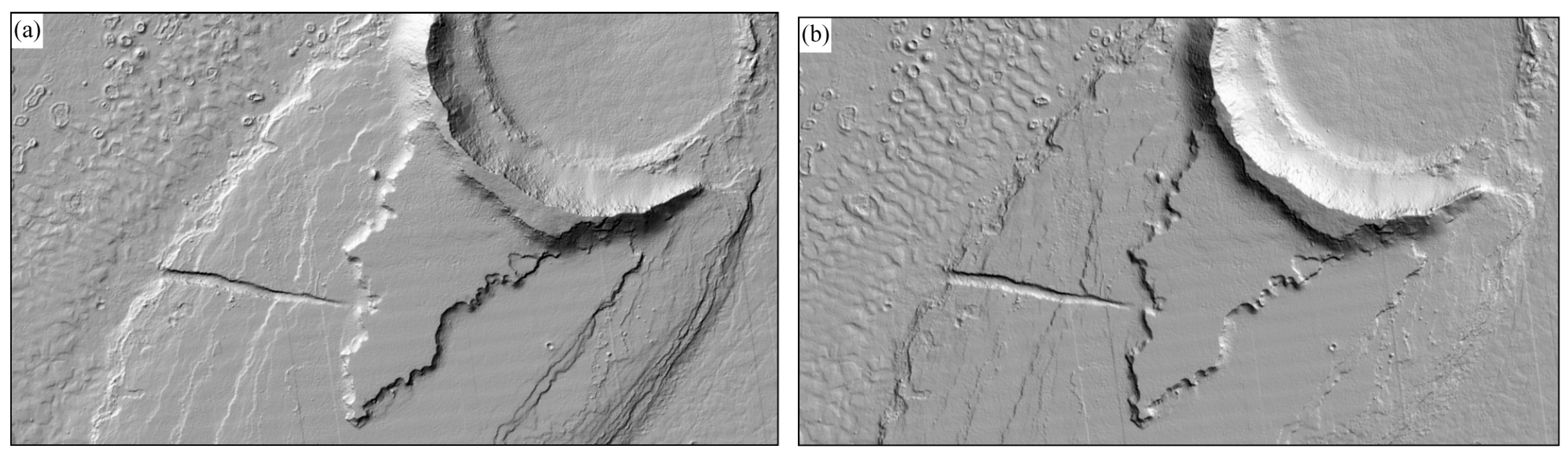
Standard analytical hill-shading is easy to compute and interpret. Its basic assumption is that the relief is a Lambertian surface illuminated by direct light from a fictive light source at an infinitive distance (the light beam has a constant azimuth and elevation angle for the entire area). The computed gray value is proportional to the cosine of the illumination incidence angle on the relief surface—the angle between the surface normal and the light beam. Areas perpendicular to the light beam are the most illuminated, while areas with an incidence angle equal or greater than 90° are in a shade. Direct illumination restricts the visualization in dark shades and brightly lit areas, where no or very little detail can be perceived. A single light beam also fails to unveil linear structures that lie parallel to it (Figure 1) which can be problematic in some applications, for example, in archaeology [20]. As a solution, Brassel [21] proposed to locally adapt the position of the illumination source in problematic areas. Imhof [22] suggested local variations in the aspect and the inclination of the global illumination vector by angles of maximum 30°. This reveals details in ridges and valleys oriented parallel to the primary direction of illumination.

Producing multiple outputs by illuminating a surface from multiple directions enhances visualization of the relief morphology. Hill-shaded images are sometimes used to guide ground surveys, but comparing multiple images in the field is extremely inconvenient. A step towards an improved understanding of the results is combining multiple shadings by considering only the mean [23], or the maximum, for each individual pixel. A common example is also a combination of standard hill-shading (315° azimuth) with vertical illumination [22,23]. Hill-shades from three different directions can also be used to create an RGB image [20,24].

Figure 1. Angle dependence of analytical hill-shading: 315° azimuth illumination (a), and 45° azimuth (b). Note the lower right corner of both plates where the relief structures have a main direction of about 45°. Almost no relief details can be observed in (b) because the structures lie in the direction of shading. The image shows ring and cone structures, and dunes in Athabasca Valles, Mars (data from HiRISE instrument aboard Mars Reconnaissance Orbiter [1]; credits to NASA/JPL/University of Arizona).

Figure 1. Angle dependence of analytical hill-shading: 315° azimuth illumination (a), and 45° azimuth (b). Note the lower right corner of both plates where the relief structures have a main direction of about 45°. Almost no relief details can be observed in (b) because the structures lie in the direction of shading. The image shows ring and cone structures, and dunes in Athabasca Valles, Mars (data from HiRISE instrument aboard Mars Reconnaissance Orbiter [1]; credits to NASA/JPL/University of Arizona).

Another approach to visualize the relief is employing a uniform diffuse illumination. Diffuse illumination was considered in the field of computer graphics (video games, photorealistic rendering) already in the 1990s when Zhukov et al. [25] introduced obscurances. The technique aims at physical representation of diffuse illumination. Ambient occlusion, which is a simplified version of the obscurances, provides more control of the appearance and has been widely used in recent years (e.g., [26,27,28]). Diffuse illumination has also been considered in cartography and GIS. Yokoyama et al. [29] described openness—a method that is based on estimating the mean horizon elevation angle (in eight directions) within a defined search radius. Openness is actually a proxy for a diffuse relief illumination. In the published article, the authors focused on the interpretation of the basic relief features and did not elaborate the physical background and the optimal visualization parameters. Kennelly and Stewart [30] showed that using a uniform sky illumination enhances the perception of the relative height of surface elements.

Both mentioned articles lack a clear explanation on how to set up the diffuse illumination to produce informative and aesthetic relief maps. We therefore advanced the idea of diffuse illumination by:

• elaborating the effect of search radius:
• elaborating the effect of number of search directions;
• elaborating the effect of other possible visualization options like spatial resolution; and
• critically comparing the proposed sky-view factor (SVF) based visualization to the analytical hill-shading.

3. Definition of Sky-View Factor

In order to overcome the drawbacks of the existing visualization techniques, for example, directional illumination problems in analytical hill-shading, we propose a visualization method based on diffuse illumination. We suggest the use of a fictive light source that illuminates the relief surface from a celestial hemisphere. This hemisphere is centered at the point being illuminated. Additionally we assume that:

• the hemisphere is equally bright across its entire area;
• there is no additional directional illumination source;
• the Earth’s curvature is neglected over short (not more than 10 km) distances.

In such a case, the relief illumination is correlated to a portion of the visible sky that is limited by the relief horizon. A point on a ridge is brighter than a point at the bottom of a steep valley because both are illuminated from the bright sky and a larger part of the sky can be seen from the ridge than from the valley. Thus we consider the share of the sky visible from each point to be a proxy for the relief illumination.

The most convenient measure for expressing the part of the visible sky is the solid angle Ω. This is a measure of how large an object appears to an observer. The solid angle of an object is proportional to area A of the object’s projection onto the unity sphere centered at the observation point. The solid angle of the (celestial) hemisphere is:

$$\Omega ={\displaystyle \underset{0}{\overset{2\pi }{\int }}{\displaystyle \underset{0}{\overset{\pi /2}{\int }}\text{cos}\varphi \cdot d\varphi \cdot d\lambda }}=2\pi .$$

(1)

φ stands for the latitude and λ for the longitude angle of the hemisphere. If we assume that above a horizontal surface, the horizon has the same vertical elevation angle in all directions, then the visible sky is limited by the surface of a cone that corresponds to the following solid angle:

$$\Omega ={\displaystyle \underset{0}{\overset{2\pi }{\int }}{\displaystyle \underset{\gamma }{\overset{\pi /2}{\int }}\text{cos}\varphi \cdot d\varphi \cdot d\lambda }}=2\pi \cdot \left(1-\text{sin}\gamma \right).$$

(2)

γ stands for the elevation angle of the relief horizon. If the horizon is not of equal height in all directions, the solid angle can be efficiently computed by observing the horizon vertical elevation angle γ_i in a chosen number of directions (Figure 2):

$$\Omega ={\displaystyle \sum _{i=1}^n{\displaystyle \underset{{\gamma }_i}{\overset{\pi /2}{\int }}\text{cos}\varphi \cdot d\varphi }}=2\pi \cdot \left(1-\frac{{\displaystyle \sum _{i=1}^n\text{sin}{\gamma }_i}}{n}\right).$$

(3)

n stands for the number of directions used to estimate the vertical elevation angle of the relief horizon. The vertical elevation angle γ_i can be computed from the horizontal distance and the elevation difference between the horizon and the vantage point. If we normalize the above defined solid angle by 2π we derive a quantity that we call the sky-view factor (SVF) [31]:

$$SVF=1-\frac{{\displaystyle \sum _{i=1}^n\text{sin}{\gamma }_i}}{n}.$$

(4)

SVF ranges between 0 and 1 (an example is shown in Figure 3). Values close to 1 mean that almost the entire hemisphere is visible, which is the case in exposed features (planes and peaks), while values close to 0 are present in deep sinks and lower parts of deep valleys from where almost no sky is visible. SVF is a physical quantity (if we do not manipulate elevation data by vertical exaggeration), especially relevant in energy balance studies (e.g., [31,32,33,34,35,36]). In general, the surface changes its temperature faster when a high share of the sky is visible; several studies investigated the correlation between SVF and heat islands within a city [37] or between frost and roads [38]. SVF is also important for the estimation of diffuse solar radiation—areas with a high SVF receive more diffuse solar radiation coming from the bright sky than areas that see only a small portion of the sky [39,40].

Figure 2. The sky-view factor is defined by the part of the visible sky (Ω) above a certain observation point as seen from a two-dimensional representation (a). The algorithm computes the vertical elevation angle of the horizon γ_i in n (eight are presented here) directions to the specified radius R (b).

Figure 2. The sky-view factor is defined by the part of the visible sky (Ω) above a certain observation point as seen from a two-dimensional representation (a). The algorithm computes the vertical elevation angle of the horizon γ_i in n (eight are presented here) directions to the specified radius R (b).

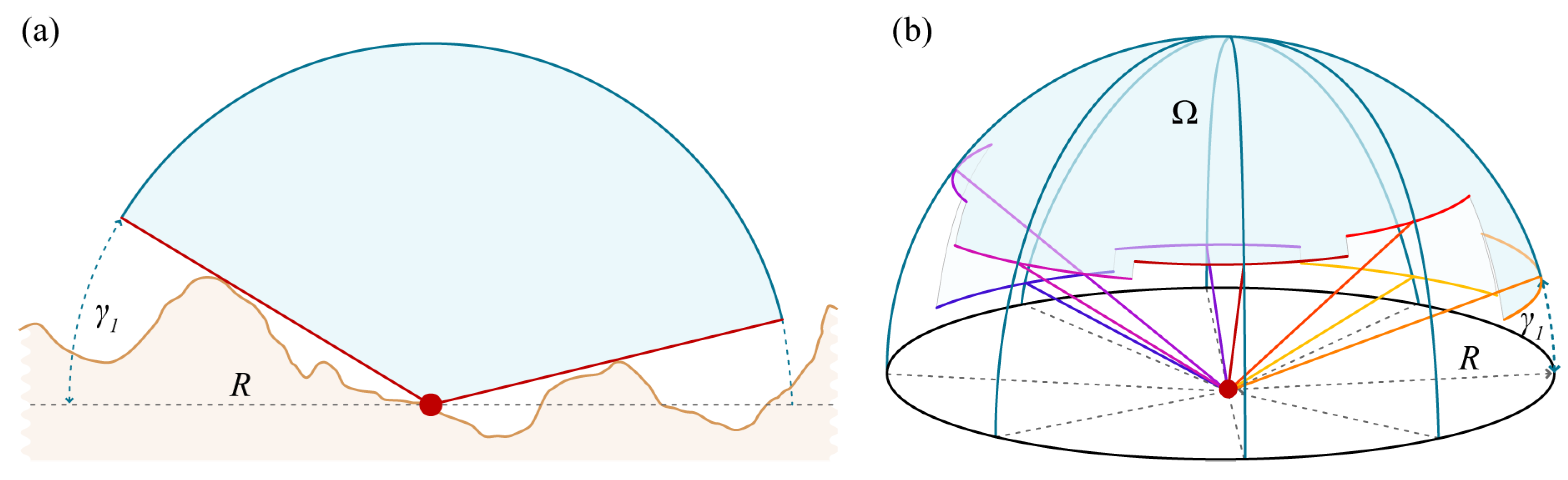
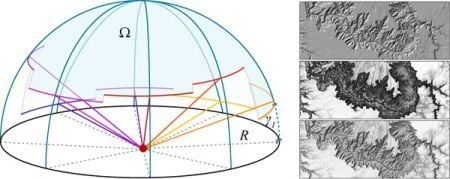
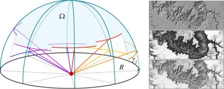
Figure 3. An example of the SVF based visualization for the volcanic region in Tanzania. Olmoti (below left), Embagai (in the middle) and small Kerimasi craters (above right) are visible. We tested visualizations based on a celestial hemisphere (a) and a celestial sphere (b). When considering the whole sphere, the results have an increased range (SVF can theoretically reach a value of 2). This brings improvement in automatic detection of linear structures because the method exposes many edges. The results however, are not intuitive because slopes are visualized in the same manner as a horizontal plane. Therefore, it is difficult to distinguish between them.

Figure 3. An example of the SVF based visualization for the volcanic region in Tanzania. Olmoti (below left), Embagai (in the middle) and small Kerimasi craters (above right) are visible. We tested visualizations based on a celestial hemisphere (a) and a celestial sphere (b). When considering the whole sphere, the results have an increased range (SVF can theoretically reach a value of 2). This brings improvement in automatic detection of linear structures because the method exposes many edges. The results however, are not intuitive because slopes are visualized in the same manner as a horizontal plane. Therefore, it is difficult to distinguish between them.

The SVF based relief visualization is a horizon determination problem similar to the openness proposed by Yokohama et al. [29]. Positive openness equal to the mean zenith angle of all determined horizons (Yokohama et al. [29] suggest also the negative openness which is based on nadir angles). Openness does not limit the estimation of each zenith angle by the mathematical horizon (as SVF does). In other words, openness considers the whole sphere and not only the celestial hemisphere like SVF. Therefore, the maximum value of openness can be greater than 90°. In addition, a plane (a long slope or a horizontal plane) without any obstacles will always have an openness of 90°. Therefore, interpreting the openness results is sometimes difficult because a slope is visualized in the same manner as a horizontal plane. Using an appropriate histogram stretch, it is possible to visualize openness in the same way as SVF, but only in the concave areas (with horizon zenith angles in all search directions less than 90°). In other areas, the methods give significantly different results. For example, Figure 3 gives an example of SVF estimated for the celestial hemisphere (a) and for the whole sphere (b). SVF in Figure 3(b) visualizes the relief as almost identical to openness. We can therefore conclude that openness is not as intuitive as SVF based visualization, but it is more appropriate in automatic detection of linear structures because the method exposes many edges.

4. Optimizing Parameters for SVF Based Visualization

The main parameters that influence an SVF based relief visualization are the number of horizon search directions and the maximum search radius. It additionally depends on the spatial resolution of the DEM, vertical exaggeration and histogram stretch. In this section we analyze how these parameters influence the results. As SVF determination is computationally demanding, the choice of optimal parameters is especially important when working with large datasets.

We implemented the SVF based relief visualization in the remote sensing software ENVI+IDL [41]. The software is publicly available and can be downloaded from [42]. It is fast enough for most visualization purposes (Table 1). For testing, we used a laptop computer running Microsoft Windows 7 (64 bit) with 2.4 GHz Intel i5 processor and 4 GB of RAM. The number of search directions and search radius determine the number of estimated horizons that is linearly correlated to the computation time. The size of the dataset is currently the limiting factor—according to our experience a computer with only 1 GB of RAM can be efficiently used for computing the SVF on the DEM of no more that 20 million pixels. The visualization of larger datasets is about ten-times slower because the computer uses the swap file.

Table 1. Sky-view factor computation speed.

Input DEM	Columns	Lines	Dir. number	Radius[pixels]	Horizons number	Processing time [min:s]
Lidar 0.5 m (Kobarid, SLO)	1,501	841	8	10	82.7 × 106	00:02.1
HiRISE 3 m (Mars)	2,241	2,824	16	20	1715× 106	00:36.5
ASTER 30 m (Ngorongoro)	5,001	5,001	8	10	1687 × 106	00:41.9

Table 1. Sky-view factor computation speed.

Input DEM	Columns	Lines	Dir. number	Radius[pixels]	Horizons number	Processing time [min:s]
Lidar 0.5 m (Kobarid, SLO)	1,501	841	8	10	82.7 × 106	00:02.1
HiRISE 3 m (Mars)	2,241	2,824	16	20	1715× 106	00:36.5
ASTER 30 m (Ngorongoro)	5,001	5,001	8	10	1687 × 106	00:41.9

4.1. Number of Search Directions

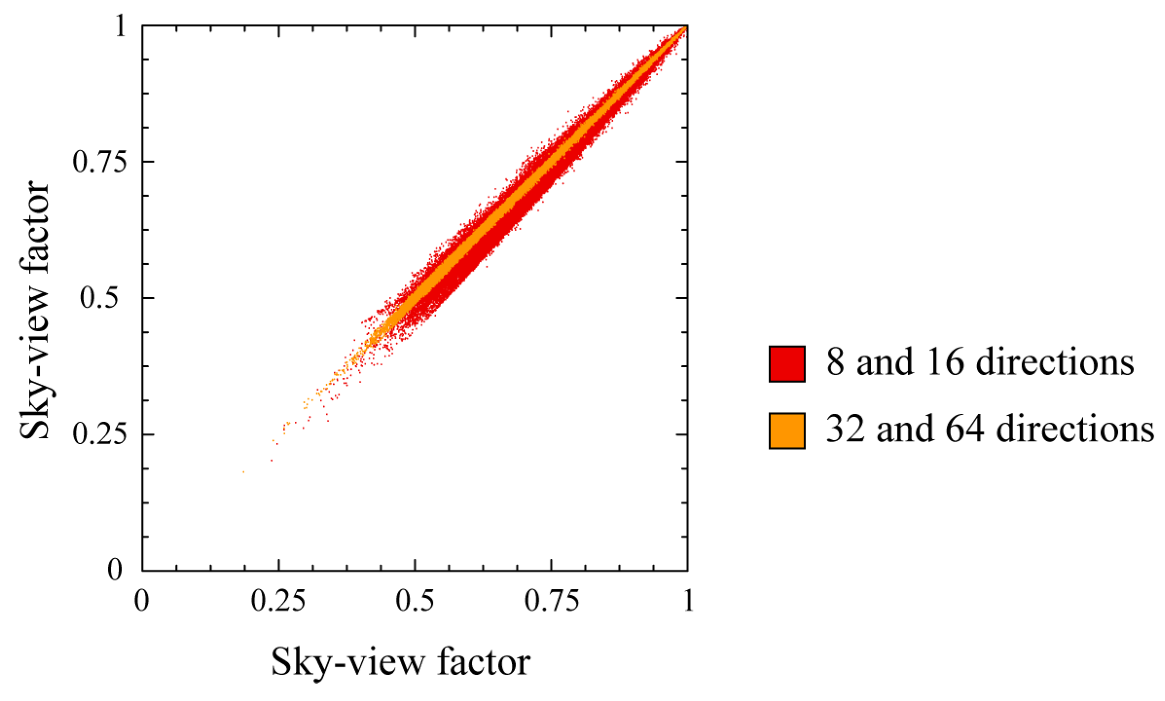
The first parameter in the computation is the number of search directions. We have evaluated SVF determined in 8, 16, 32 and 64 directions, both visually and statistically. A visual comparison reveals that objects are detectable in all results; however some minor differences can be seen on the edges of convex objects when 8 or 64 directions are chosen. The statistical analysis was performed on the area of archaeological site Tonovcov grad in Slovenia, on a DEM with a 0.5 m spatial resolution and vertical accuracy of 20 cm (1,501 × 841 pixels), and a search radius of 10 m (20 pixels).

Scatterplots in Figure 4 show a comparison of SVFs estimated in 8 and 16 directions, and 32 and 64 directions. The scatterplots show that the number of directions has no systematic influence on SVF. With a higher number of search directions the difference decreases and there is no significant deviation between SVF estimated in 32 or 64 directions.

Figure 4. Scatterplots comparing SVF estimated in 8 and 16 directions (red), and 32 and 64 directions (yellow).

Figure 4. Scatterplots comparing SVF estimated in 8 and 16 directions (red), and 32 and 64 directions (yellow).

The optimal number of directions for SVF estimation also depends on the search radius; at a radius of merely 1 pixel, the exact number of directions is 8 and it makes no sense to compute it in more directions. We recommend that at least 8 directions should be chosen at any time. For visualization purposes, more than 32 search directions bring no noticeable improvement. This corresponds to the findings of Dozier et al. [43] who developed a fast algorithm for horizon determination; they suggest that 32 search directions are enough in radiation studies. We also made some simulations to estimate the accuracy of the computed SVF. Considering the error propagation of elevation data accuracy in SVF computation, number of search directions, search radius and computation speed, we additionally suggest that the following rule of thumb should be applied: do not use fewer directions than half of the search radius (in pixels), but also not more than the value of the search radius—e.g., a reasonable number of search directions for a search radius of 20 pixels is between 10 and 20.

4.2. Maximum Search Radius

An SVF based visualization exposes large relief features when a large search radius is chosen and detailed features when a small radius is used. A scatterplot in Figure 5(a) compares SVF estimated for a search radius of 5 m (10 pixels) versus 20 m (40 pixels) (for the same area as in Figure 4). SVF reaches its true (i.e., lowest) value at the real (mathematical) horizon. All obstacles in front of the real horizon are lower than the real horizon. Therefore SVF estimated with a search radius of, for example, 20 m cannot be larger than SVF estimated with a 5 m radius. This is confirmed in Figure 5(b) that compares profiles computed with a radius of 5 m, 10 m, and 20 m; SVF is systematically reduced with an increase in the search radius.

Figure 5. The scatterplot (a) compares sky-view factor estimated for a 5 m (10 pixels) versus 20 m (40 pixels) search radius (for the same area as in Figure 4). Profile (b) across SVF computed with a 5 m, 10 m, and 20 m search radius.

Figure 5. The scatterplot (a) compares sky-view factor estimated for a 5 m (10 pixels) versus 20 m (40 pixels) search radius (for the same area as in Figure 4). Profile (b) across SVF computed with a 5 m, 10 m, and 20 m search radius.

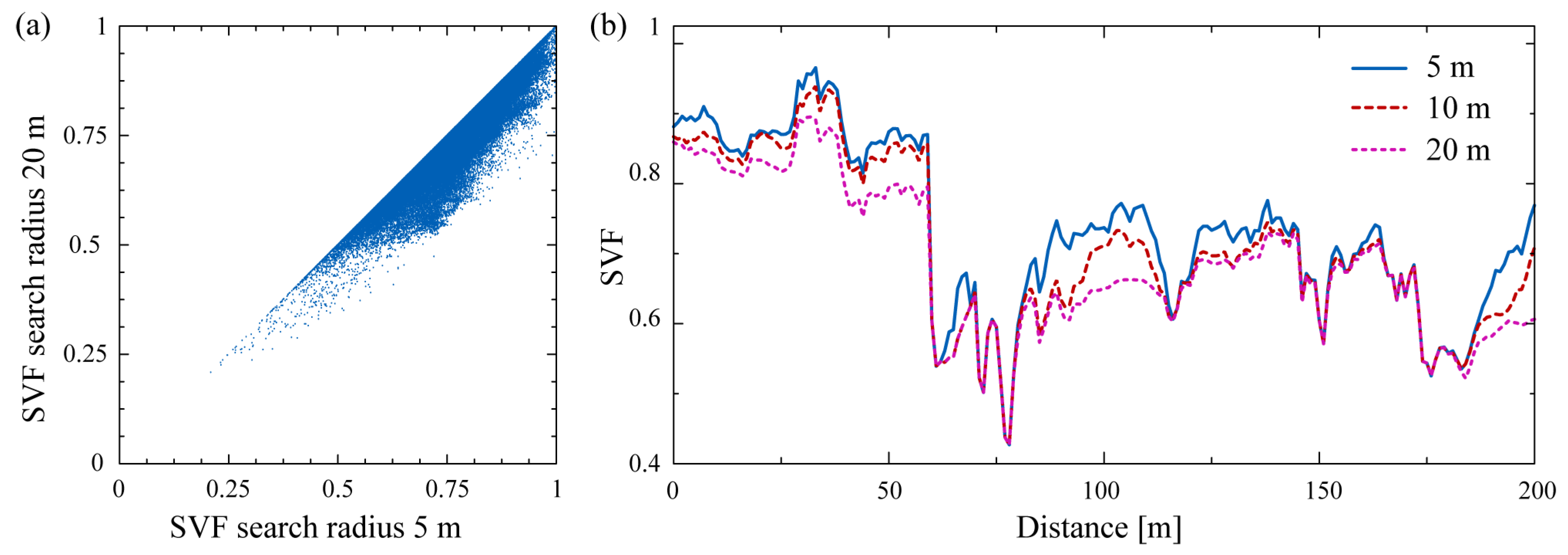
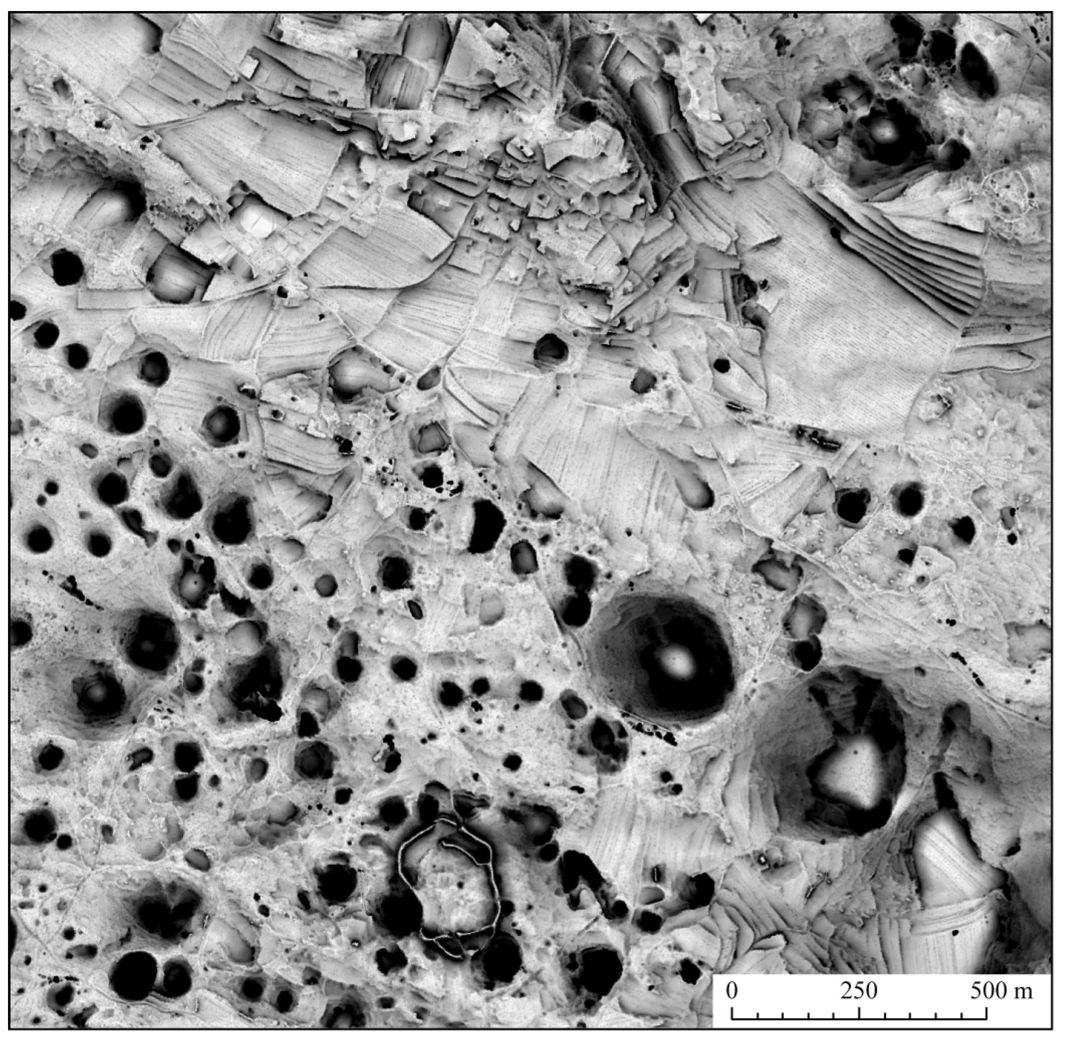
Figure 6 shows an example of how to choose the appropriate search radius. The area lies in the south-western Slovenia and is karstic with numerous dolines. The objective of this visualization was to map all dolines in the area. Most of them have a diameter that does not exceed 50 m and they are approximately 10 m deep. We have therefore chosen a search radius of 30 m (30 pixels) and most dolines can indeed be clearly visible as black spots. The two largest dolines in the lower right have a diameter of almost 100 m and no obstacle can be detected on the flat bottom in their centers, so they are visualized as a “doughnut”. The selected search radius also reveals agricultural terraces (upper right), archaeological remains (lower centre) and some stone walls.

Figure 6. Visualization of dolines in a karstic area (Slovenia). The elevation model has a spatial resolution of 1 m. SVF was computed in 16 directions and a search radius of 30 m was used (similar to the diameter of the dolines).

Figure 6. Visualization of dolines in a karstic area (Slovenia). The elevation model has a spatial resolution of 1 m. SVF was computed in 16 directions and a search radius of 30 m was used (similar to the diameter of the dolines).

In order to choose the optimal search radius one should consider the size of the objects to be visualized or any other characteristic distances in the relief (as described for the example above). A search radius ranging between 10 and 30 pixels is usually a good choice for general visualization purposes. According to our experience, a search radius greater than 50 pixels does not make sense because of the significant increase in computation time.

4.3. Spatial Resolution

Just like every other raster analysis, SVF determination depends on the spatial resolution of the input. Downsampling the input DEM is a preferred option in the case of a large search radius because the lower resolution DEM corresponds (pixel wise) to a smaller search radius. In cases with extremely large search radius (with medium and low resolution data), the Earth’s curvature and projection properties can have a significant effect on the results (at a distance of 10 km, the curvature combined with the atmospheric refraction affects the elevation by about 7 m).

5. Comparison with Other Visualization Techniques

In this section we compare the performance of SVF based visualization with other visualization techniques. We first concentrate on a comparison with analytical hill-shading. According to our experience, this standard visualization method performs best in a moderately hilly relief. Very steep valley slopes lead to problems on the south-eastern slopes (assuming that the illumination comes from the northwest); when the angle between the illumination ray and the normal to the relief is greater than 90°, the cosine of the incidence angle is negative. Just the positive values are accepted in analytical hill-shading and consequently all negative values are presented with the same color as null (black), yielding to saturation. No details can be observed in the case of steep south-eastern slopes. It appears as if all were in a shadow. According to our experience, it is impossible to distinguish relief details (without any significant gray values histogram manipulations) on a slope steeper than 30° if this slope faces a direction opposite to the illumination source. The saturation can be reduced if a higher elevation angle of the light source is used. However, this also decreases the shading effect.

The SVF based visualization performs significantly better than hill-shading when the relief changes gradually, without sharp edges. In this case an analytically shaded image does not reveal enough details; the horizontal surface has an incidence angle that equals the illumination elevation angle while the steepest slopes (e.g., 10°) have an incidence angle only a few degrees larger or smaller. This means that the horizontal area is always in the middle of the gray value range and the resulting image has no contrast. Gray value histogram can always be manipulated but an average GIS user rarely does so, hence it is important that the visualization has an appropriate histogram range. SVF visualizes gradual relief mostly by the light gray values that make the relief features easier to recognize. In addition, all “anomalies”—such as steep valleys—are “marked” by darker color tones.

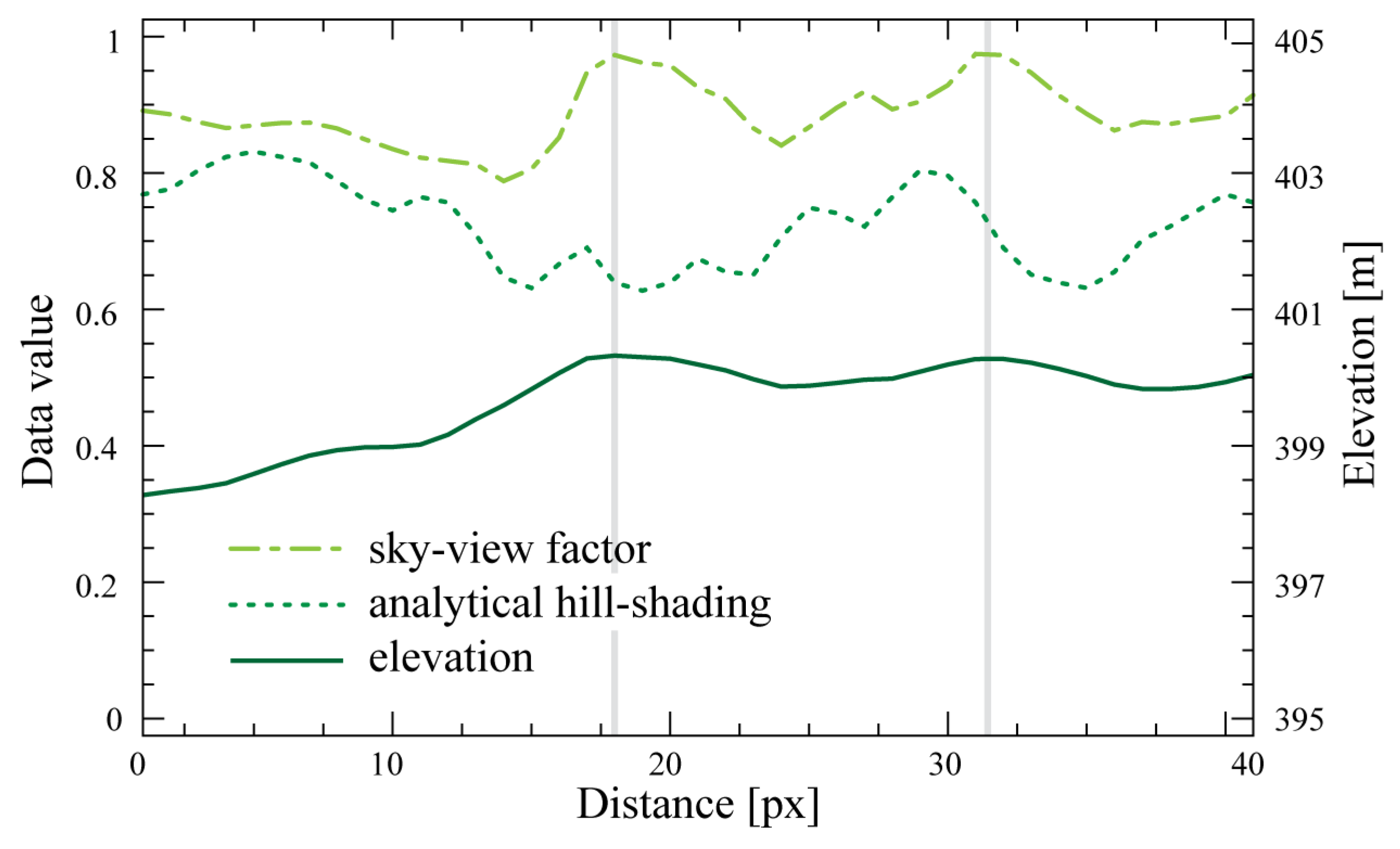
Figure 7 shows transects (profiles) of analytical hill-shading and SVF compared to the elevation data for Tonovcov grad, Slovenia. It can be observed that the relief changes gradually over the entire transect; remains of the building walls, about half a meter high, are marked by vertical lines. The position of the profile can be seen in Figure 8 as a red line. The hill-shading of this profile is relatively noisy; a small change in the relief aspect or slope can significantly change the hill-shading value. It would be possible to estimate the hill-shading from a larger computation window or from a downsampled DEM in order to remove the noise. However, doing this would also likely remove the details we want to see. This is the advantage of SVF based visualization—it is robust because it is estimated from a relatively large computation window but it still preserves many details. SVF contains less noise and thus performs better in visualizing the archaeological remains.

Figure 7. A 20 m long profile of DEM created from laser scanning data over the archaeological site at Tonovcov grad (Slovenia); see Figure 8 for the profile position. We compare values of SVF (range 0 to 1), analytical hill-shading (cosine of incidence angle, 0 to 1) and elevation (395 to 405 m). We also tested transects extending in other directions to consider the effect of directional illumination, but the results of analytical hill-shading were always noisier than the SVF.

Figure 7. A 20 m long profile of DEM created from laser scanning data over the archaeological site at Tonovcov grad (Slovenia); see Figure 8 for the profile position. We compare values of SVF (range 0 to 1), analytical hill-shading (cosine of incidence angle, 0 to 1) and elevation (395 to 405 m). We also tested transects extending in other directions to consider the effect of directional illumination, but the results of analytical hill-shading were always noisier than the SVF.

We have compared both techniques on numerous areas visualizing data with resolution ranging between 0.5 and 200 m. Here we show the following examples: a high-resolution DEM of the archaeological site at Tonovcov grad (Figure 8), and a moderate resolution DEM of the Grand Canyon, USA (Figure 9). As a drawback SVF based visualization does not provide such a plastic representation of the relief surface as hill-shading. In order to achieve the best visual interpretation it therefore makes sense to combine both techniques (e.g., with the use of a transparent overlay; Figure 9). A similar approach was already proposed by Kennelly [44] who combined relief hill-shading and curvature. As curvature considers only the closest pixels, our tests indicate that a combination of hill-shading and SVF based visualization is more effective.

Although the standard analytical hill-shading is the most used technique for relief visualization, it is not the only one. Some applications of solar isolation [45] showed that their results are more efficient because the illumination source (the Sun) moves. This movement partially removes the issue of direct illumination. But the computation is slow and it is thus more appropriate to combine the analytical hill-shading from multiple directions, e.g., equally spaced between 0 and 360°. Combining multiple shading layers by considering only the mean or the maximum of an individual pixel represents a step towards an improved understanding of the results (Figure 10(b)). The results are intuitive and similar to the SVF based visualization, but, in our experience, reveal fewer details.

Figure 8. A comparison of analytical hill-shading (a) and SVF based visualization (b) of a DEM generated from lidar data (0.5 m spatial resolution), for the archaeological site at Tonovcov grad (Slovenia). The remains of the building outlines and defense walls are clearly recognizable on the SVF based visualization. The profile location from Figure 7 is represented by the red line. SVF was computed in 16 directions with a 10 m search radius.

Figure 8. A comparison of analytical hill-shading (a) and SVF based visualization (b) of a DEM generated from lidar data (0.5 m spatial resolution), for the archaeological site at Tonovcov grad (Slovenia). The remains of the building outlines and defense walls are clearly recognizable on the SVF based visualization. The profile location from Figure 7 is represented by the red line. SVF was computed in 16 directions with a 10 m search radius.

Figure 9. Even though the rugged relief is appropriately represented by hill-shading, as shown in (a), the legibility of its features is enhanced with the use of SVF (b), and even more so when both methods are combined (c). The combination is especially suitable for cartographic purposes. Grand Canyon, Arizona, USA. Data source USGS (1” NED). SVF was computed in 16 directions with a 300 m search radius.

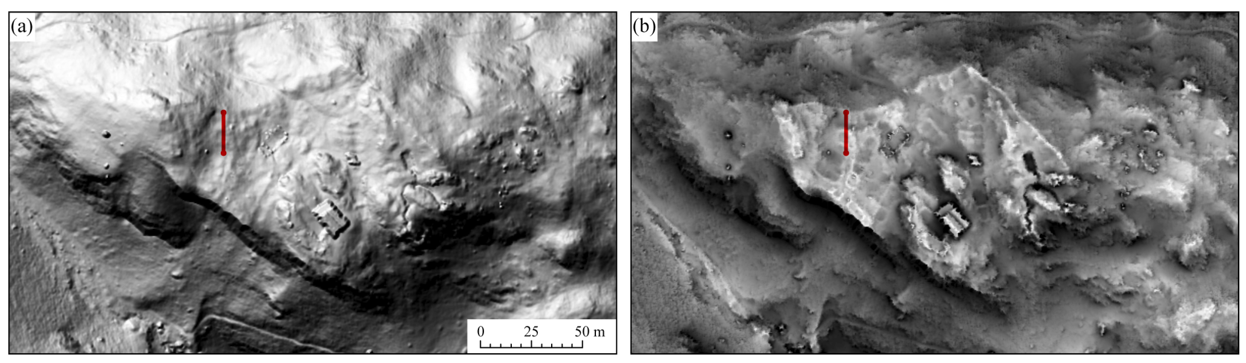
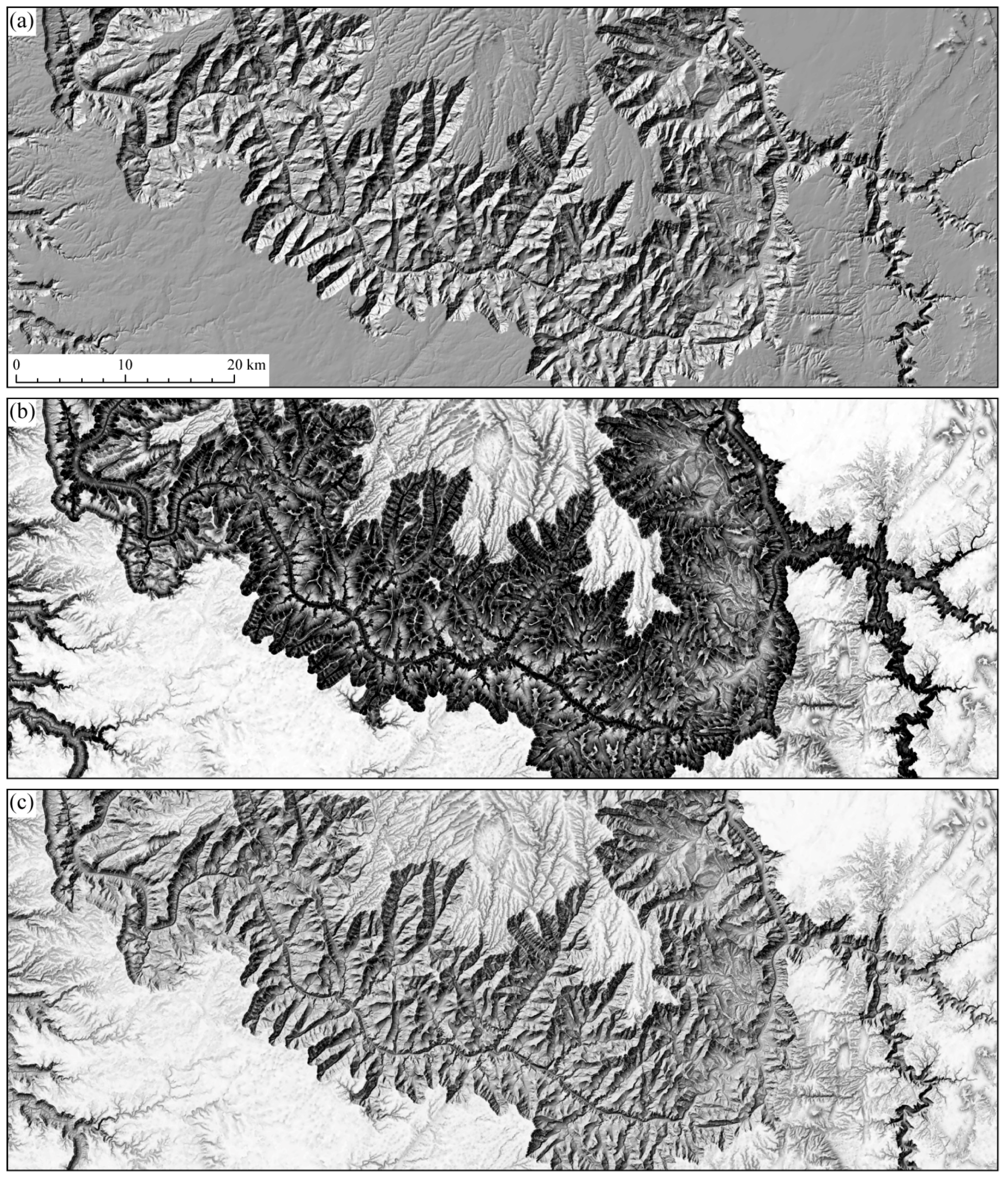
Figure 9. Even though the rugged relief is appropriately represented by hill-shading, as shown in (a), the legibility of its features is enhanced with the use of SVF (b), and even more so when both methods are combined (c). The combination is especially suitable for cartographic purposes. Grand Canyon, Arizona, USA. Data source USGS (1” NED). SVF was computed in 16 directions with a 300 m search radius.

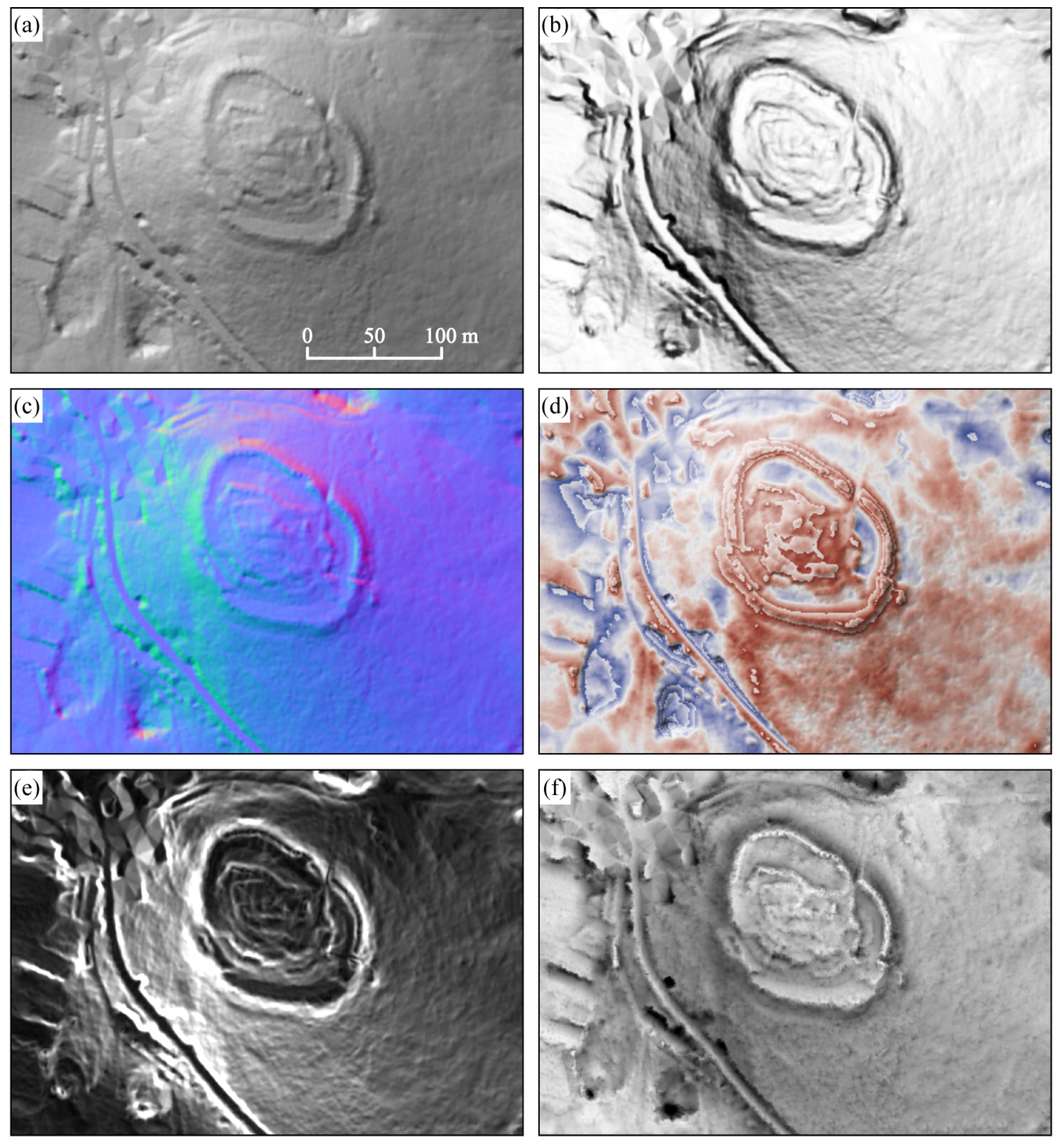
Figure 10. A comparison of visualization techniques used in archaeological interpretation for the area of Zagrajec Hill Fort, near Komen, Slovenia, a known yet un-excavated site. The images are produced by: standard analytical hill-shading (45° zenith angle, 315° azimuth; (a)); the mean of analytical hill-shadings from 16 directions (b); a RGB composite of the first three components of the principal component analysis of analytical hill-shadings from 16 directions (c); trend removal and height coding by modulo distribution (±1 m, (d)); Sobel edge detection (e); sky-view factor (10 m search radius in 16 directions, (f)).

Figure 10. A comparison of visualization techniques used in archaeological interpretation for the area of Zagrajec Hill Fort, near Komen, Slovenia, a known yet un-excavated site. The images are produced by: standard analytical hill-shading (45° zenith angle, 315° azimuth; (a)); the mean of analytical hill-shadings from 16 directions (b); a RGB composite of the first three components of the principal component analysis of analytical hill-shadings from 16 directions (c); trend removal and height coding by modulo distribution (±1 m, (d)); Sobel edge detection (e); sky-view factor (10 m search radius in 16 directions, (f)).

Because images created by illumination from several angles are highly correlated (the same scene is viewed) it is possible to mathematically transform them with the Principal Component Analysis (PCA) that “summarized” the information [20]. The first three components usually contain a high percentage (typically over 99 %) of the information or variability in the original dataset. They can thus be expected to provide a basis for the visualization of all the shade direction data with minimal loss of archaeological features. The PCA components analysis—especially the combination of the first and second principal components, or the RGB composite of the first three components—simplifies the interpretation of the multiple shading data (Figure 10(c)). However it does not provide consistent results with different datasets and is less appropriate than SVF based visualization on those datasets where, e.g., circular (especially concave, i.e., quarries) features are questionable [8].

Height coding with modulo distribution [46] dissects the area into equally high elevation bands and colors them according to the height within each band. The color coding interval scheme is repeated in every band interval. This technique reveals the small differences within a flat landscape, while the bands can be interpreted as contours on a steep and diverse terrain. It is very illustrative for the discrimination of, for example, palaeochannels, especially when preceded by trend removal (Figure 10(d)). If the trend is removed, the method gives similar results as the local relief model technique [47]. The problem of both methods is that although they reveal many features they are less intuitive than SVF and analytical hill-shading because larger landscape features are not presented [8].

For the problem of unintuitive results, the Sobel filter (Figure 10(e)) can be used to search perceptible edges in DEM. Other spatial analyses can be used to enhance the concave or convex features, and edges of morphological features. For interpretation purposes, the visualization usually combines the results with analytically shaded relief.

6. Applications of SVF

SVF can be efficiently used in numerous studies where digital elevation model visualizations and automatic feature extraction techniques are indispensable, e.g., in geography, geomorphology, cartography, hydrology, glaciology, forestry and disaster management. It can be used even in engineering applications, such as, predicting the availability of the GPS signal in urban areas. In this section three possible applications outside the visualization field will be briefly described.

The first example is relief morphology classification. Using SVF estimated with multiple search radii, one can relatively easily determine the rank of relief features as regards their importance: from globally important structures to local structures. If this is combined with the results of Yokohama et al. [29], who proposed to compute also the mean depression angle, all significant relief structures can be extracted.

SVF is also extremely important for estimating the effect of topography on the solar irradiation received by the surface (e.g., [48,49]). The diffuse part of solar irradiation is linearly correlated to the SVF of the true horizon (assuming isotropic diffuse irradiation). In order to estimate the true horizon, a larger search radius has to be considered. Due to the average visibility (considering fog or smog) and relief morphology (in general only peaks and ridges have a more distant horizon), the radius can generally be limited to 10 km. With a longer search radius, the effect of the Earth’s curvature has to be considered.

In numerous cities, the effect of an urban heat island (UHI) [37] is an important issue. UHI is correlated to the radiative and convective cooling. The radiative cooling is more efficient in areas with large SVF because these areas can radiate their energy unobscured into the space. The convective cooling depends on the urban geometry. In general it is more efficient in the areas with large SVF because they are exposed to the large volume of (usually cooler) surrounding air. In order to study this, UHI scientists retrieved SVF from fish-eye lens images that are only suitable for estimating SVF at a single point [31]. With this proposed method, SVF can be computed from a digital surface model (e.g., laser scanning based). A small search radius can be used for convective cooling studies. In addition, the SVF range can be extended from the hemisphere to the entire sphere, thus increasing the range from 0–1 to 0–2.

7. Conclusion

Analytical hill-shading is a visualization method that considers the neighboring (closest) pixels to estimate the relief slope and aspect that are required to compute the incidence angle of the light source. It is therefore mostly useful for representing sharp relief edges. However, the optimal way to describe the gradual elevation anomalies is not through the use of a method that describes a pixel by its local slope and aspect, but a method that shows the context of the pixel within its further surroundings. In these cases, it and its derivatives (e.g., PCA visualization of hill-shading from different azimuths), are not as successful as SVF based visualization. The ability to consider the neighbourhood context makes SVF an outstanding tool also when compared to other visualization techniques used in archaeology. Some of them also consider the larger neighborhood (e.g., local relief model) but are not intuitive. This is because all the larger features are removed so one can see only anomalies in respect to the relief trend.

SVF is appropriate for general visualizations of natural heritage. The concave forms (e.g., dolines in karstic relief, impact or volcanic craters) stand out as dark regions. SVF based visualization gives a much better impression on the relative elevation of each point. It is therefore also possible to see all small ridges in a relatively flat relief. The search radius is the parameter that determines how relief features will be visualized using SVF. One can choose a large search radius and the most important features on the global scale will be clearly visible. In visualizations of cultural heritage, large search radii (over 20 pixels assuming lidar DEM with 1 m spatial resolution) are a good option to visualize mining traces, hollow ways and agricultural terraces. These line features are usually narrower than the suggested search radius, so they stand out in the visualization as dark lines. If a small search radius is chosen, the local details will stand out. In the lidar data it is even possible to see the noise in the data if a radius of 2–5 pixels is chosen (assuming a DEM with a resolution of about 1 m). For the remote sensing of cultural heritage it is more important that burial mounds, remains of ancient buildings, and ridge-and-furrow can be successfully visualized using a small radius, especially when vertical exaggeration of 2–3 is used. However, these features—visualized as white lines surrounded by gray values—are not as clear as the concave ones.

References

- Kirk, R.L.; Howington-Kraus, E.; Rosiek, M.R.; Anderson, J.A.; Archinal, B.A.; Becker, K.J.; Cook, D.A.; Galuszka, D.M.; Geissler, P.E.; Hare, T.M.; et al. Ultrahigh resolution topographic mapping of Mars with MRO HiRISE stereo images: Meter-scale slopes of candidate Phoenix landing sites. J. Geophys. Res. 2008, 113, E00A24. [Google Scholar] [CrossRef]
- Burrough, P.A.; McDonnell, R.A. Principles of Geographical Information Systems, 2nd ed.; Oxford University Press: Oxford, UK, 1998. [Google Scholar]
- Amante, C.; Eakins, B. ETOPO1 1 Arc-Minute Global Relief Model: Procedures, Data Sources and Analysis; Technical Memorandum NESDIS NGDC-24; NOAA: Boulder, CO, USA, 2009. Available online: http://www.ngdc.noaa.gov/mgg/global/global.html (accessed on 9 July 2010).
- ASTER GDEM Validation Team. ASTER GDEM Validation Summary Report; 2009. Available online: https://lpdaac.usgs.gov/lpdaac/content/download/4009/20069/version/3/file/ASTER+GDEM+Validation+Summary+Report.pdf (accessed on 9 July 2010).
- Zakšek, K.; Podobnikar, T.; Oštir, K. Solar radiation modelling. Comput. Geosci. 2005, 31, 233–240. [Google Scholar] [CrossRef]
- Jain, M.K.; Singh, V.P. DEM-based modelling of surface runoff using diffusion wave equation. J. Hydrol. 2005, 302, 107–126. [Google Scholar] [CrossRef]
- Chaplot, V. Impact of DEM mesh size and soil map scale on SWAT runoff, sediment, and NO3-N loads predictions. J. Hydrol. 2005, 312, 207–222. [Google Scholar] [CrossRef]
- Kokalj, Ž.; Zakšek, K.; Oštir, K. Application of sky-view factor for the visualization of historic landscape features in lidar-derived relief models. Antiquity 2011, 85, 263–273. [Google Scholar] [CrossRef]
- Horn, B. Hill shading and the reflectance map. Proc. IEEE 1981, 69, 14–47. [Google Scholar] [CrossRef]
- Jenny, B. An interactive approach to analytical relief shading. Cartographica 2001, 38, 67–75. [Google Scholar] [CrossRef]
- Patterson, T. A desktop approach to shaded relief production. Cartogr. Perspect. 1997, 28, 38–40. [Google Scholar] [CrossRef]
- Patterson, T.; Hermann, M. Creating value-enhanced shaded relief in Photoshop. Available online: http://www.shadedrelief.com/value/value.html (accessed on 9 July 2010).
- Price, W. Relief presentation: Manual airbrushing combined with computer technology. Cartogr. J. 2001, 38, 107–112. [Google Scholar] [CrossRef]
- Phong, B.T. Illumination for computer generated pictures. Commun. ACM 1975, 18, 311–317. [Google Scholar] [CrossRef]
- Blinn, J.F. Models of light reflection for computer synthesized pictures. SIGGRAPH Comput. Graph. 1977, 11, 192–198. [Google Scholar] [CrossRef]
- Batson, R.; Edwards, E.; Eliason, E. Computer generated shaded relief images. J. Res. US Geol. Surv. 1975, 3, 401–408. [Google Scholar]
- Minnaert, M. Photometry of the moon. In Planets and Satellites; Kuiper, G.P., Middlehurst, B.M., Eds.; The University of Chicago Press: Chicago, IL, USA, 1961; pp. 213–248. [Google Scholar]
- Yoëli, P. Analytische Schattierung. Ein kartographischer Entwurf. Kartographische Nachrichten 1965, 15, 141–148. [Google Scholar]
- Devereux, B.J.; Amable, G.S.; Crow, P. Visualisation of LiDAR terrain models for archaeological feature detection. Antiquity 2008, 82, 470–479. [Google Scholar] [CrossRef]
- Brassel, K. A model for automatic hill-shading. Cartogr. Geogr. Inf. Sci. 1974, 1, 15–27. [Google Scholar] [CrossRef]
- Imhof, E. Cartographic Relief Presentation; Walter de Gruyter: Berlin, Germany, 1982. [Google Scholar]
- Hobbs, K.F. The rendering of relief images from digital contour data. Cartogr. J. 1995a, 32, 111–116. [Google Scholar] [CrossRef]
- Hobbs, K.F. An investigation of RGB multi-band shading for relief visualisation. Int. J. Appl. Earth Obs. Geoinf. 1999b, 1, 181–186. [Google Scholar] [CrossRef]
- Zhukov, S.; Iones, A.; Korin, G. An Ambient Light Illumination Model. In Proceedings of Eurographics Rendering Workshop on Rendering Techniques, Vienna, Austria, 29 June–1 July 1998; pp. 45–55.
- Méndez-Feliu, À.; Sbert, M. From obscurances to ambient occlusion: A survey. Visual Comput. 2009, 25, 181–196. [Google Scholar] [CrossRef]
- González, F.; Sbert, M.; Feixas, M. Viewpoint-based ambient occlusion. IEEE Comput. Graph. Applications 2008, 28, 44–51. [Google Scholar] [CrossRef]
- Ruiz, M.; Szirmay-Kalos, L.; Umenhoffer, T.; Boada, I.; Feixas, M.; Sbert, M. Volumetric ambient occlusion for volumetric models. Visual Comput. 2010, 26, 687–695. [Google Scholar] [CrossRef]
- Yokoyama, R.; Shlrasawa, M.; Pike, R.J. Visualizing topography by openness: A new application of image processing to digital elevation models. Photogramm. Eng. Remote Sensing 2002, 68, 251–266. [Google Scholar]
- Kennelly, P.J.; Stewart, A.J. A uniform sky illumination model to enhance shading of terrain and urban areas. Cartogr. Geogr. Inform. Sci. 2006, 33, 21–36. [Google Scholar] [CrossRef]
- Steyn, D. The calculation of view factors from fisheye-lens photographs. Atmos. Ocean 1980, 18, 254–258. [Google Scholar] [CrossRef]
- Häntzschel, J.; Goldberg, V.; Bernhofer, C. GIS-based regionalisation of radiation, temperature and coupling measures in complex terrain for low mountain ranges. Meteorol. Appl. 2005, 12, 33–42. [Google Scholar] [CrossRef]
- Richards, K. Sky view and weather controls on nocturnal surface moisture deposition on grass at urban sites. Phys. Geogr. 2006, 27, 70–85. [Google Scholar] [CrossRef]
- Oke, T.R. Boundary Layer Climates, 2nd ed.; Routledge: London, UK, 1988. [Google Scholar]
- Marks, D.; Dozier, J.; Davis, R. A clear-sky longwave radiation model for remote alpine areas. Arch. Met. Geoph. Biokl. Serie B 1979, 27, 159–187. [Google Scholar] [CrossRef]
- Eliasson, I. Urban nocturnal temperatures, street geometry and land use. Atmos. Environ. 1996, 30, 379–392. [Google Scholar] [CrossRef]
- Bourbia, F.; Awbi, H.B. Building cluster and shading in urban canyon for hot dry climate: Part 1: Air and surface temperature measurements. Renewable Energy 2004, 29, 249–262. [Google Scholar] [CrossRef]
- Blennow, K. Modelling minimum air temperature in partially and clear felled forests. Agr. Forest Meteorol. 1998, 91, 223–235. [Google Scholar] [CrossRef]
- Robinson, D. Urban morphology and indicators of radiation availability. Solar Energy 2006, 80, 1643–1648. [Google Scholar] [CrossRef]
- Yard, M.D.; Bennett, G.E.; Mietz, S.N.; Coggins, L.G., Jr.; Stevens, L.E.; Hueftle, S.; Blinn, D.W. Influence of topographic complexity on solar insolation estimates for the Colorado River, Grand Canyon, AZ. Ecol. Model. 2005, 183, 157–172. [Google Scholar] [CrossRef]
- ITT Visual Information Solutions. ENVI Software: Image processing & analysis solutions. 2010. Available online: http://www.ittvis.com/ProductServices/ENVI.aspx (accessed on 9 November 2009).
- IAPS ZRC SAZU, Institute of Anthropological and Spatial Studies ZRC SAZU. Sky-View Factor. 2010. Available online: http://iaps.zrc-sazu.si/index.php?q=en//node/138 (accessed on 9 December 2010).
- Dozier, J.; Bruno, J.; Downey, P. A faster solution to the horizon problem. Comput. Geosci. 1981, 7, 145–151. [Google Scholar] [CrossRef]
- Kennelly, P.J. Terrain maps displaying hill-shading with curvature. Geomorphology 2008, 102, 567–577. [Google Scholar] [CrossRef]
- Challis, K.; Forlin, P.; Kincey, M. A generic toolkit for the visualisation of archaeological features on airborne lidar elevation data. Archaeol. Prospect. 2011. in print. [Google Scholar] [CrossRef]
- Wood, J. The Geomorphological Characterization of Digital Elevation Models. Ph.D. Thesis, University of Leicester, Leicester, UK, 1996. Available online: http://www.soi.city.ac.uk/~jwo/phd (accessed on 7 December 2009). [Google Scholar]
- Hesse, R. LiDAR-derived Local Relief Models—A new tool for archaeological prospection. Archaeol. Prospect. 2010, 17, 67–72. [Google Scholar] [CrossRef]
- Corripio, J.G. Vectorial algebra algorithms for calculating terrain parameters from DEMs and solar radiation modelling in mountainous terrain. Int. J. Geogr. Inf. Sci. 2003, 17, 1–23. [Google Scholar] [CrossRef]
- Revfeim, K.J.A. A simple procedure for estimating global daily radiation on any surface. J. Appl. Meteorol. 1978, 17, 1126–1131. [Google Scholar] [CrossRef]
© 2011 by the authors; licensee MDPI, Basel, Switzerland. This article is an open access article distributed under the terms and conditions of the Creative Commons Attribution license (http://creativecommons.org/licenses/by/3.0/).
Share and Cite
MDPI and ACS Style
Zakšek, K.; Oštir, K.; Kokalj, Ž. Sky-View Factor as a Relief Visualization Technique. Remote Sens. 2011, 3, 398-415. https://doi.org/10.3390/rs3020398
AMA Style
Zakšek K, Oštir K, Kokalj Ž. Sky-View Factor as a Relief Visualization Technique. Remote Sensing. 2011; 3(2):398-415. https://doi.org/10.3390/rs3020398
Chicago/Turabian StyleZakšek, Klemen, Kristof Oštir, and Žiga Kokalj. 2011. "Sky-View Factor as a Relief Visualization Technique" Remote Sensing 3, no. 2: 398-415. https://doi.org/10.3390/rs3020398