Roughness Mapping on Various Vertical Scales Based on Full-Waveform Airborne Laser Scanning Data

Abstract

Roughness is an important input parameter for modeling of natural hazards such as floods, rock falls and avalanches, where it is basically assumed that flow velocities decrease with increasing roughness. Seeing roughness as a multi-scale level concept (i.e., ranging from fine-scale soil characteristics to description of understory and lower tree layer) various roughness raster products were derived from the original full-waveform airborne laser scanning (FWF-ALS) point cloud using two different types of roughness parameters, the surface roughness (SR) and the terrain roughness (TR). For the calculation of the SR, ALS terrain points within a defined height range to the terrain surface are considered. For the parameterization of the SR, two approaches are investigated. In the first approach, a geometric description by calculating the standard deviation of plane fitting residuals of terrain points is used. In the second one, the potential of the derived echo widths are analyzed for the parameterization of SR. The echo width is an indicator for roughness and the slope of the target. To achieve a comparable spatial resolution of both SR layers, the calculation of the standard deviation of detrended terrain points requires a higher terrain point density than the SR parameterization using the echo widths. The TR describes objects (i.e., point clusters) close but explicitly above the terrain surface, with 20 cm defined as threshold height value for delineation of the surface layer (i.e., forest floor layer). Two different empirically defined vegetation layers below the canopy layer were analyzed (TR I: 0.2 m to 1.0 m; TR II: 0.2 m to 3.0 m). A 1 m output grid cell size was chosen for all roughness parameters in order to provide consistency for further integration of high-resolution optical imagery. The derived roughness parameters were then jointly classified, together with a normalized Digital Surface Model (nDSM) showing the height of objects (i.e., trees) above ground. The presented approach enables the classification of forested areas in patches of different vegetation structure (e.g., varying soil roughness, understory, density of natural cover). For validation purposes in situ reference data were collected and cross-checked with the classification results, positively confirming the general feasibility of the proposed vertical concept of integrated roughness mapping on various vertical levels. Results can provide valuable input for forest mapping and monitoring, in particular with regard to natural hazard modeling.

1. Introduction

For the modeling of natural hazards, such as avalanches [1], rock falls [2] and floods [3], information about the roughness of the Earth’s surface is an essential input. Basically, it can be assumed that flow velocities decrease with increasing roughness [4]. However, for all of these different processes, roughness can be seen in various scale levels, ranging from fine-scale soil characteristics to terrain and landscape features. On the micro-level, roughness is described in a range of millimeters to centimeters. Relevant parameters in that context are land cover types, such as herbaceous and grass vegetation. Relevant meso-level roughness features include objects and vegetation in a range of decimeters to meters, such as shrubs and boulders. The macro-level is determined by topography and terrain features, where the scale ranges from one to hundred meters [5].

In state-of-the-art avalanche modeling approaches, empirically developed roughness schemes based on a set of varying land cover types are implemented [6,7,8]. Such land cover classification can consist of, for example, (1) screes and boulders, (2) shrubs or mountain pines, (3) herbaceous and grass vegetation including low bushes, and (4) compact grassland or solid rock. Depending on the exposition, various skid factors are derived from these surface types (see Table 1) [8]. Surface roughness is relevant for glide avalanches on micro-level as well as for snow slabs on meso- and macro-level. The estimated skid factors are introduced in snow gliding and snow pressure modeling [9].

In the field of hydrology, surface roughness is introduced in runoff models for detecting superficial flow velocities and water depths [10,11]. The practical assessment of roughness is thereby typically based on a coarse surface and vegetation classification. Markart et al. [12] identified six thematic classes ranging from very smooth to very rough. Different types of vegetation can span several roughness classes. In particular this applies to forest locations, where surface roughness is dependent on specific low-vegetation cover.

Table 1. Skid factors assigned to land cover types featuring varying roughness characteristics [8].

Land cover class		Range	Skid factor
1	Screes and boulders	>30 cm	1.2–1.3
2	Shrubs or mountain pines Mounds with vegetation cover Cattle treading Screes	>1 m >50 cm 10–30 cm	1.6–1.8
3	Grass vegetation incl. low bushes Fine debris mixed with vegetation Small mounds with vegetation cover Grass vegetation incl. superficial cattle treading	<1 m <10 cm <50 cm	2.0–2.4
4	Compact grassland Solid rock Fine debris mixed with soil Moist sinks		2.6–3.2

Table 1. Skid factors assigned to land cover types featuring varying roughness characteristics [8].

Land cover class		Range	Skid factor
1	Screes and boulders	>30 cm	1.2–1.3
2	Shrubs or mountain pines Mounds with vegetation cover Cattle treading Screes	>1 m >50 cm 10–30 cm	1.6–1.8
3	Grass vegetation incl. low bushes Fine debris mixed with vegetation Small mounds with vegetation cover Grass vegetation incl. superficial cattle treading	<1 m <10 cm <50 cm	2.0–2.4
4	Compact grassland Solid rock Fine debris mixed with soil Moist sinks		2.6–3.2

Accordingly, further parameters are needed for classification. For example, for virgin soils the dominance of migrating plants is relevant. For grassland roughness characteristics are strongly affected by land use (e.g., pasturing, ski slopes, hay meadows). In moist locations the moss rate is crucial, while for areas with bushes particularly, the type of plant cover is relevant.

The current standard way of assessing surface roughness is using empirical methods based on data collected in the field [12]. Taking the macro-level as example, terrain features are described approximately via wavelength and amplitude of sinusoids [13]. Roughness assessment on meso- and micro-level can be carried out by fitting ductile slats to the surface [14]. All these methods require on-site inspections which becomes extremely time-consuming and costly for large-area assessments.

In general, remote sensing offers the advantage of an area-wide standardized survey and is expected to deliver roughness assessments in comparable accuracy. Especially airborne laser scanning (ALS), also referred to as airborne LiDAR, has been proven as the state of the art technology for the acquisition of high precision topographic information. As an active remote sensing technique, ALS is able to capture the topography with high precision even for densely forested areas. The transmitted nanosecond-long (e.g., 4 ns) laser pulses in the near-infrared range of wavelengths (e.g., 1.0 μm or 1.5 μm) have a typical beam divergence of 0.5 mrad, resulting in footprint diameters of 0.2 m to 0.5 m for typical flying heights above ground of 400 m to 1,000 m. Due to the high pulse repetition frequency of up to 400 kHz a high sampling rate on the ground can be achieved, which allows the description of the terrain surface in decimeter scale. For example, Smith, et al. [15] have shown that terrain or landscape roughness in the macro-level can be determined from digital terrain model (DTM) analyses. Furthermore, Straatsma and Baptist [16] have demonstrated the potential of ALS in combination with multi-spectral remote sensing data for floodplain roughness parameterization in the meso-level.

This special issue paper is based on two conference papers of Aubrecht et al. [17] and Hollaus and Höfle [18] and aims at assessing the full potential of ALS points cloud and full-waveform (FWF) data for assessing two different roughness parameters, i.e., the terrain roughness (TR) and the surface roughness (SR). For the parameterization of the SR, two different approaches are analyzed using the 3D point distribution and the echo width derived from FWF-ALS data respectively. As described in Wagner et al. [19], the echo width is an indicator for roughness and the slope of the target. Therefore, the potential of the derived echo widths are analyzed for roughness characterization. For the parameterization of the TR 3D, points close, but explicitly above, the terrain surface are analyzed to assess the near terrain vertical vegetation structure. For the mapping of the vertical vegetation structure, the calculated roughness layers are used as input. We see roughness as a multi-scale level concept, i.e., ranging from fine-scale soil characteristics to description of understory and lower tree level. Results of the presented ‘vertical roughness mapping’ concept can be valuable input for forest monitoring, in particular with regard to natural hazard modeling. The derived terrain roughness layers as well as the vertical roughness maps are presented and discussed.

2. Study Areas and Data

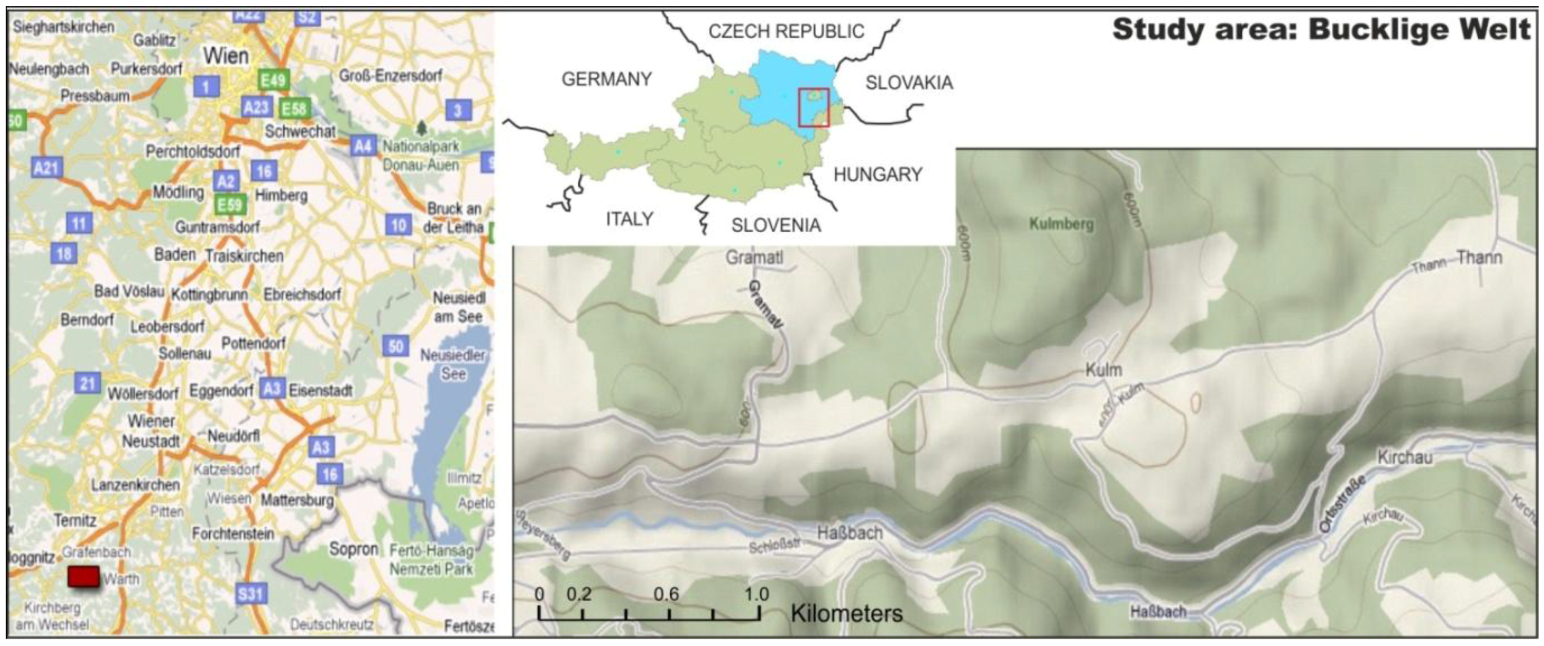
2.1. Study Areas

The study area Bucklige Welt, covering approximately 10 square kilometers, is located in the so-called Bucklige Welt, a hilly region in the south-eastern part of Lower Austria (about 70 km south of the Vienna basin) also known as ‘land of the 1,000 hills’ (Figure 1). Widely dominated by forest of varying characteristics (i.e., deciduous, coniferous, and mixed forest), Bucklige Welt is a typical rural area dominated by agricultural land interrupted by a few small settlements (e.g., Haßbach, Kirchau, Kulm). In line with the overall characteristics of the Bucklige Welt region, the study site, which belongs to the municipal area of Warth, features hilly terrain conditions with maximal 300 meters elevation difference.

The study area Wienerwald is located in the western part of Vienna (Figure 2), in the so-called Wienerwald (Vienna Woods), and covers about 200 hectares forest and a small part of an urban area. The study area is part of the UNESCO biosphere reserve Wienerwald, which was defined by the provinces of Lower Austria and Vienna in 2005.

Figure 1. Study area Bucklige Welt, Lower Austria (UTM33N, LE: 578100, 5277900, UR: 582800, 5279900).

Figure 1. Study area Bucklige Welt, Lower Austria (UTM33N, LE: 578100, 5277900, UR: 582800, 5279900).

Figure 2. Overview of the study area Wienerwald located at the western border of the city Vienna (UTM33N, LE: 590450, 5341300, UR: 592450, 5342350). In the subareas 1–4 additional analyses are done (see Section 3.1).

Figure 2. Overview of the study area Wienerwald located at the western border of the city Vienna (UTM33N, LE: 590450, 5341300, UR: 592450, 5342350). In the subareas 1–4 additional analyses are done (see Section 3.1).

Since the 19th century, the Vienna Woods region has been used as a traditional recreation area for Viennese and residents of Lower Austria, living in the vicinity. In general, the landscape of the Vienna Woods is characterized by individual deciduous forest stands, which are closely interlinked with meadows while the forests are dominated by oak and hornbeam, beech at higher altitudes, and ash in the peak region of north-facing slopes. The forests are characterized by a balanced age class distribution (tree ages vary between 5 and 180 years) and with tree heights varying between 2 m and 45 m. The clearings are partly covered by very dense brushwood, i.e., blackberry. Furthermore, there are some young forest stands covered with very dense red beech (Fagus sylvatica). Further details of the study area can be found in Hollaus, et al. [20].

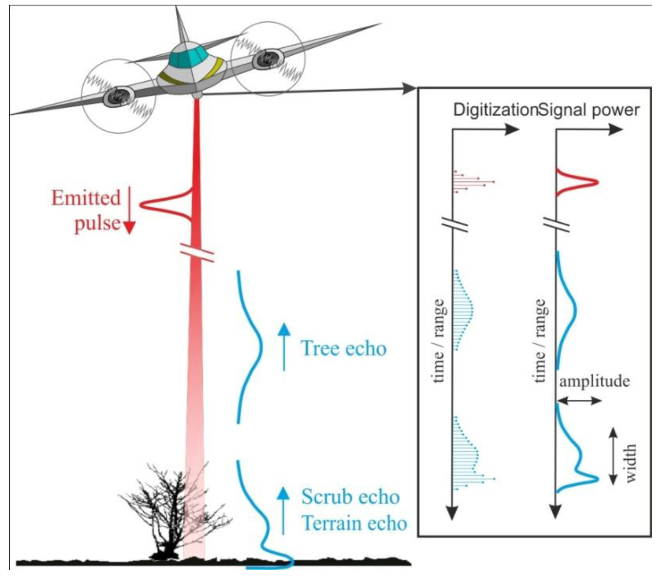
2.2. Airborne Laser Scanning Data

For both study areas a full waveform Airborne Laser Scanning (FWF-ALS) system (Riegl LMS-Q560) was used to acquire the topographic data. The data acquisitions were done in the framework of commercial terrain mapping projects, fully covering the Federal State of Lower Austria and the city of Vienna. The ALS data was provided by the “Amt der Niederösterreichischen Landesregierung, Gruppe Baudirektion, Abteilung Vermessung und Geoinformation“ and by the city of Vienna (MA41 Stadtvermessung) for the study area Bucklige Welt and Wienerwald respectively. For both study areas the FWF-ALS data was captured under leaf-off conditions and without snow cover.

For the study area Bucklige Welt, the FWF-ALS data was delivered as XYZ coordinate triples organized in tiles. Originally, ALS-inherent information on scan geometry, radiometric information and the trajectory was not available for this study. Therefore, the calculations of the FWF attributes echo width and amplitude were not possible. For the Wienerwald study area, strip-wise FWF-ALS data was delivered including the entire full-waveform information as well as the trajectories. For the study area Wienerwald, the pre-processing of the FWF-ALS data was done by the company AREA Vermessung ZT GmbH using Riegl software.

For the current study the geo-referenced 3D echo points and the determined attributes for each echo, i.e., the echo width and the amplitude, serve as input for the following analyses. For both study areas, the digital terrain models (DTM) were calculated using SCOP++ [21] software. For the determination of the digital surface models (DSM) the approach described in Hollaus et al. [22] was applied using the OPALS [23] software. Finally, the normalized digital surface models (nDSM) were calculated by subtracting the DTM from the DSM (Figure 2). The derived topographic models (DTM, DSM, nDSM) have a spatial resolution of 1.0 m and 0.5 m respectively (Table 2). The DTMs are used for normalizing the 3D echo points (d_z) and therefore, for the selection of terrain and near-terrain echoes. Further details of the used FWF-ALS data are summarized in Table 2.

Table 2. Characteristics of the used FWF-ALS data.

ALS data characteristics	Study Areas
	Bucklige Welt	Wienerwald
Avg. echo density (m−2)	~30	~34
Available point cloud data format	xyz	full-waveform
Period of acquisition	Spring 2007	January 2007
laser wavelength (nm)	1,550	1,550
Laser scanner system	Riegl LMS-Q560	Riegl LMS-Q560
Avg. flying height above ground (m)	~500	~500
Data acquisition company	Diamond Airborne Sensing	Diamond Airborne Sensing
DTM, DSM, nDSM resolution (m)	1.0	0.5

Table 2. Characteristics of the used FWF-ALS data.

ALS data characteristics	Study Areas
	Bucklige Welt	Wienerwald
Avg. echo density (m−2)	~30	~34
Available point cloud data format	xyz	full-waveform
Period of acquisition	Spring 2007	January 2007
laser wavelength (nm)	1,550	1,550
Laser scanner system	Riegl LMS-Q560	Riegl LMS-Q560
Avg. flying height above ground (m)	~500	~500
Data acquisition company	Diamond Airborne Sensing	Diamond Airborne Sensing
DTM, DSM, nDSM resolution (m)	1.0	0.5

2.3. Reference Data

To validate the results of the ALS based vertical roughness mapping, in situ reference data was collected during a field survey on 16 April 2009. Locations of reference points were stored using a Garmin eTrex GPS handheld model. Extensive photo documentation was an essential part of the data collection allowing capturing a certain neighborhood around fixed reference point locations. A total of 24 points were collected in the course of the field survey with focus on getting a representative point set featuring different types of vegetation including scrubs and brushwood.

3. Methods

Looking at roughness from the ALS sensing technique point of view, the spatial scale of observation plays a crucial role. Roughness with a spatial scale of up to a few decimeters cannot be determined directly by using the ALS range measurements (i.e., XYZ of point cloud) because of the range accuracy [24], which generally lies far above the given laser wavelength of a few micrometers. Hence, micro-structures can only be determined indirectly, for example, by using the strength of reflection of a laser echo (i.e., amplitude), which is correlated with target reflectivity [25] but also surface roughness [19].

Therefore, the focus of the current paper is on the derivation of roughness parameters of the meso-structure with a spatial scale of decimeters to meters using the ALS point cloud directly. Using the 3D point cloud, guarantees the maximum information content, while preserving the highest data density and not introducing any biasing decisions on suitable target raster resolution, filter or aggregation strategies [26,27]. On the end-user side however, it is much more convenient and applicable to deal with pre-processed roughness images, i.e., featuring substantially reduced amount of data and simple raster data structure, which can be processed operatively in standard GIS and remote sensing software packages. Computations of additional point cloud attributes and subsequent generalized raster layers require a sophisticated software implementation, including both the mathematical definitions and intelligent management of the large amount of data which arises when working with high density laser point data.

In the following paragraphs two different roughness parameters calculated on the basis of the initial ALS point cloud are described and the resulting raster layer products are illustrated. The first roughness parameter is named surface roughness (SR). For its calculation, all ALS terrain points within a defined height range to the terrain surface are considered. For the parameterization of the SR, two approaches are investigated. In the first approach a geometric description of the 3D point distribution of terrain points is used. In the second, the potential of the derived echo widths are analyzed for the SR characterization. The second roughness parameter is named terrain roughness (TR) and describes objects (i.e., point clusters) close but explicitly above the terrain surface, with 20 cm defined as threshold height value for delineation of the surface layer (i.e., forest floor layer). Two different empirically defined vegetation layers below the canopy layer were analyzed for this paper: (1) very low brushwood or undergrowth from 0.2 m to 1.0 m, such as bushes and shrubs (TR I), and (2) understory vegetation from 0.2 m to 3.0 m, e.g., being indicative of different tree types (TR II).

Finally, an approach is presented to map the vertical vegetation structure (i.e., roughness on various height levels inside the forest), where non-forested regions were masked out using a previously derived forest mask. This mask had been produced implementing an integrated analysis approach, considering aerial imagery and ALS data (i.e., Object-based Image Analysis, OBIA). Seeing roughness as a multi-scale level concept important for various issues in forest monitoring, the presented concept facilitates complex data handling and analysis for forest managers.

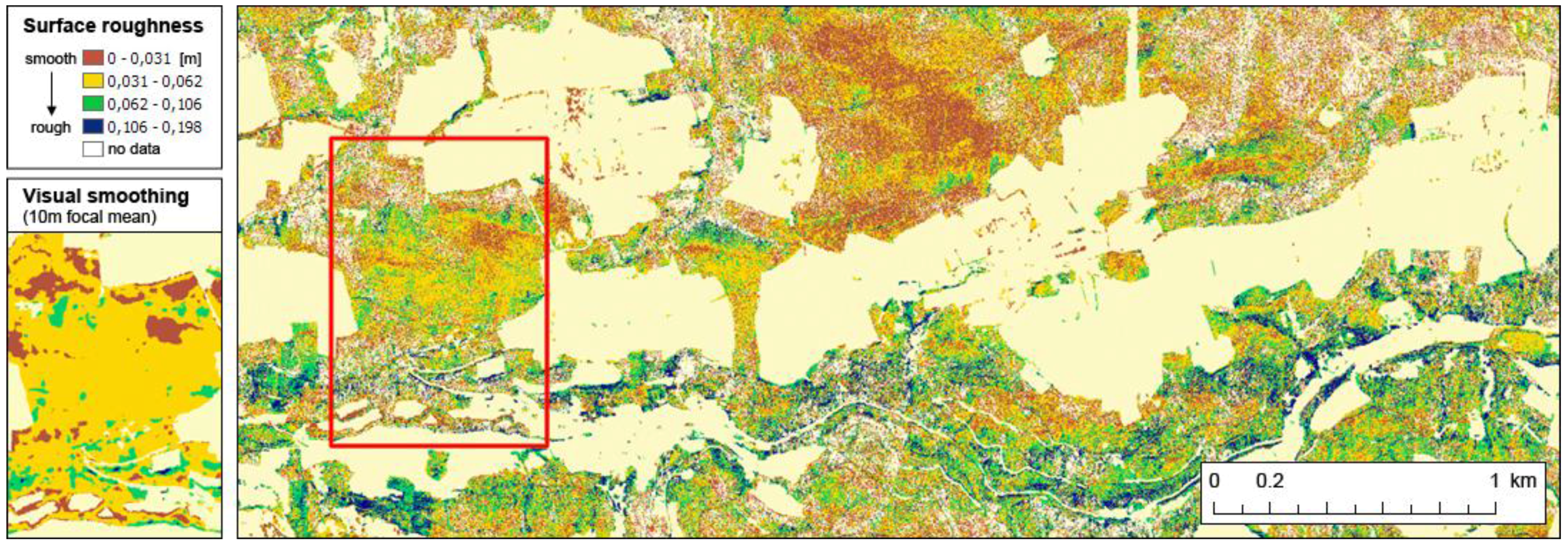
3.1. Surface Roughness

The surface roughness (SR) is parameterized (i) by the standard deviation of the plane fitting residuals of all echoes within a raster cell or a certain distance, which are located below a defined normalized height (d_z) threshold (Figure 3(a)), and (ii) by the mean echo width of the selected terrain echoes. For the current study different height thresholds (d_z = 0.20 m, 0.25 m, 0.5 m, 1.0 m) are analyzed and the results from both approaches were compared to each other. The comparison of the SR images was done for the Wienerwald test site as only here the full-waveform information of the ALS data is available.

Surface roughness was defined as small scale height variations up to a few decimeters above ground. Algorithmically, simply the standard deviation of orthogonal regression plane fitting residuals is chosen. Taking the residuals to a best fit plane can be compared to a prior detrending of the heights. The detrending of the ALS heights is important for slanted surfaces, where otherwise the computed standard deviation would increase with increasing slope (i.e., height variation), even with the surface being plane. The orthogonal regression plane fitting (Figure 3(b)) is favored over vertical fitting because for very steep surfaces, the vertical residuals can become very large, even though the plane fits very well to the points. In this sense orthogonal fitting means that the orthogonal distances from plane to points are minimized. In practice, for every laser echo the orthogonal plane fitting is performed in a local neighborhood (i.e., considering all terrain echo neighbors in a certain distance for plane computation; e.g., <1.0 m) and stored as an additional attribute to the original laser echo. Finally, the SR images were generated by averaging the standard deviations of all echoes within the raster cell with a raster size of 1.0 m. The unit of the derived SR images is in meters and can be compared between different flight epochs and ALS systems.

Figure 3. Schematic representation of roughness calculation using ALS data. (a) Predefined cube or cylinder for selecting terrain or off-terrain echoes used for plane fitting. (b) Principle of orthogonal regression plane fitting (modified from www.mathworks.com).

Figure 3. Schematic representation of roughness calculation using ALS data. (a) Predefined cube or cylinder for selecting terrain or off-terrain echoes used for plane fitting. (b) Principle of orthogonal regression plane fitting (modified from www.mathworks.com).

To improve the visual impression of the SR data, a focal neighborhood function (i.e., averaging within a circular neighborhood with a radius of 10 m) is applied to the original raster data of the Bucklige Welt test site. Using focal operations is a common form of generalization smoothing the visual impression of raster data. It is particularly valuable for identifying hot spot regions and spatial patterns in heterogeneous raster data. It is very important to decide first how to deal with existing ‘no data’ values in the input data. They can either be ignored or ‘no data’ is assigned to the output grid cell in case any of the considered neighboring cells has a ‘no data value’.

For parameterizing the SR using the echo width, one must consider that the meso-structure is defined to be smaller than the footprint diameter which is in the range of 0.5 m to 2.0 m. Such structures can be obtained either directly, if a high point density with overlapping footprints is given, or if the range resolution of the scanner system allows distinguishing multiple echoes in the magnitude of few decimeters, with the latter currently not achieved by state-of-the-art scanners. The maximum sampling interval is typically 1.0 ns, which corresponds to approximately 15.0 cm (30.0 cm for both ways) [28] of the measured range. For objects a few times larger than the sampling interval, the widening of the echo (i.e., larger echo width) indicates a certain vertical extent of the illuminated object, which can be assigned to roughness in a broader sense. For the FWF-ALS data used, the full-waveforms received were digitized with an interval of 1 ns (Figure 4). A Gaussian decomposition method was applied to estimate, in addition to the 3D position, the scattering properties of the targets i.e., the amplitude and the echo width [28]. Therefore, the derived echo width of each single echo is representative for the roughness within the illuminated footprint (Figure 4). For a laser beam with multiple echoes, the illuminated footprint area contributing to one echo decreases depending on the collision area of the previous reflected echoes.

Figure 4. Schematic representation of a FWF-ALS system. A Gaussian decomposition is applied to derive echo widths, which are used for the parameterization of surface roughness. [adapted from 29].

Figure 4. Schematic representation of a FWF-ALS system. A Gaussian decomposition is applied to derive echo widths, which are used for the parameterization of surface roughness. [adapted from 29].

Only single echoes are selected for the terrain roughness parameterization, in order to guarantee that solely extended targets with similar footprint sizes are investigated. This restriction was chosen because multiple echoes exhibit a different effective area illuminated by the laser beam contributing to the backscatter compared to area-extended targets. For this study the influence of varying flying heights and consequently varying ranges, as well as the local incidence angle are neglected because (i) the study area is small and therefore the variation in the ranges is small, (ii) the effect of the local incidence angle on the echo width is small and (iii) especially for forest floors, the estimation of the local incidence angle is associated with relative large uncertainties.

Finally, the terrain roughness layers are generated by aggregating the selected echo widths per raster cell (e.g., mean value) with a raster size of 1.0 m. The unit of the SR images is in nanoseconds and could be converted to meters. To compare the SR images derived from the standard deviation of plane fitting residuals and the mean echo widths, linear regression analyses between the SR images are applied and correlation coefficients are calculated, in order to derive a measure for the comparability of the two SR images.

For validating the surface roughness parameters for the test site Wienerwald, the derived surface roughness layers are compared to each other. A linear regression from both roughness images was calculated.

In addition to the entire image, subareas were selected, each representing an individual land cover type (see subareas in Figure 2), i.e., grass (1), bushes (2), young (3) and old (4) forest, to calculate the linear regression. Finally, a plausibility check was done carrying out field investigations. To exclude effects of varying footprint sizes caused by multiple echoes on the derived echo widths only extended targets are used. Therefore, only single echoes (i.e., extended targets) below the defined height thresholds were selected for generating additional roughness layers. It is expected that this investigation provides information about the comparability of roughness layers derived from single and multiple echoes respectively.

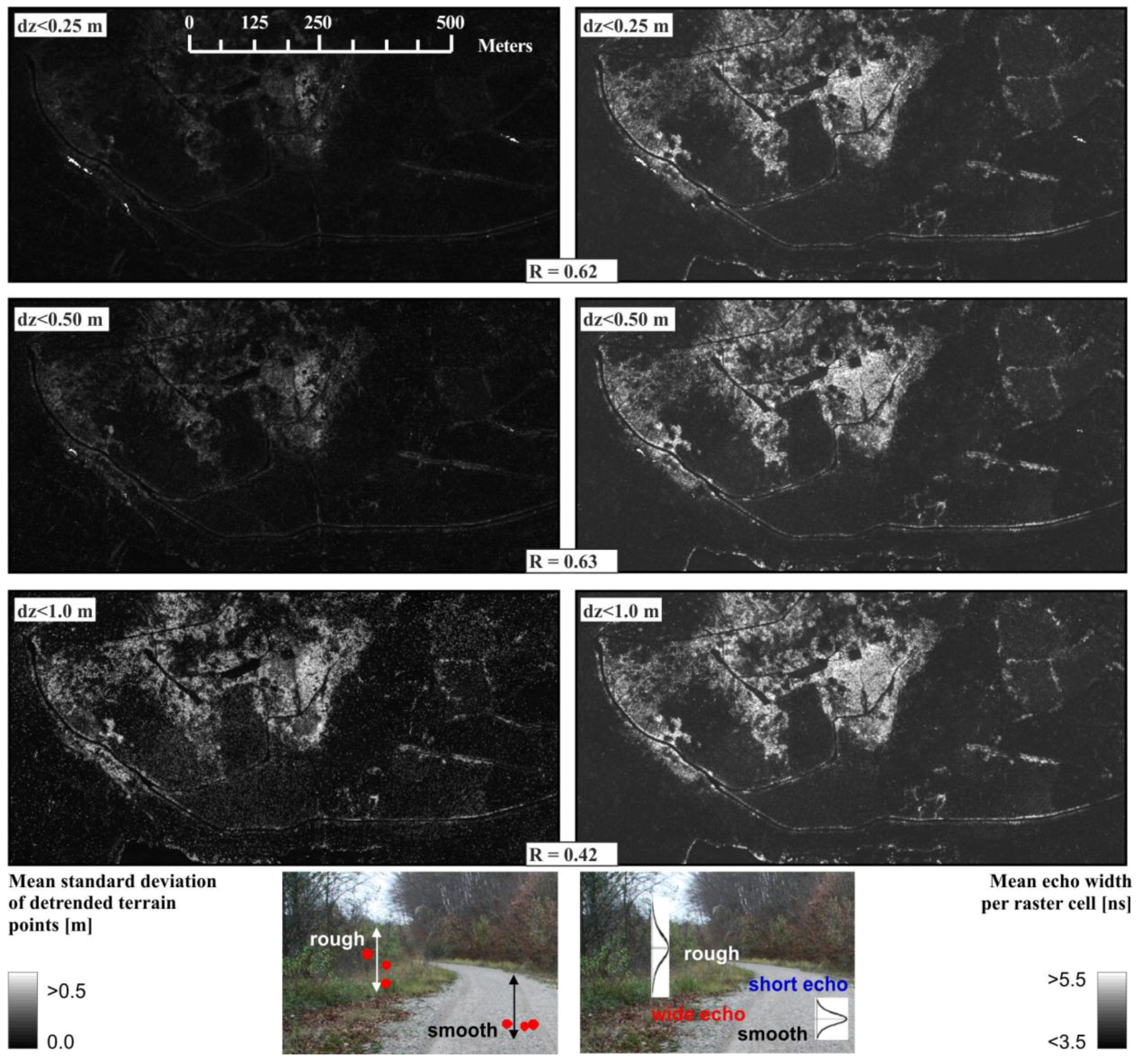
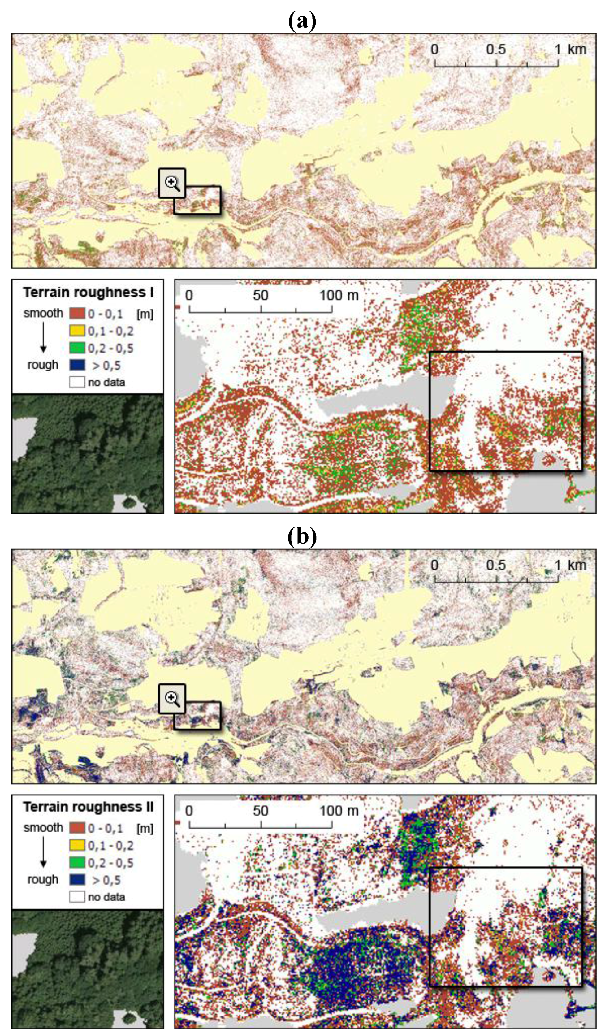
3.2. Terrain Roughness (TR)

Terrain roughness (TR) is defined as the unevenness of the terrain surface (including rocks and low vegetation) at scales of several meters. In mathematical terms this implies calculation of the standard deviation of normalized heights of non-terrain echoes within boxes of predefined size. In contrast to the SR computation, only echoes close to, but above, terrain (d_z > 0.2 m) are considered for the TR derivation. Two different vegetation layers are analyzed in this context, one considering very low brushwood or undergrowth between 0.2 m and 1.0 m (e.g., bushes and shrubs; TR I; Figure 3(a)) and the other considering understory vegetation between 0.2 m and 3.0 m (TR II; Figure 3(a)). The second layer is particularly valuable for identifying different types of trees, such as large coniferous trees with few, mostly cut branches in the lower levels or broadleaf trees with just stem and crown compared to smaller trees with branches hanging down to the ground.

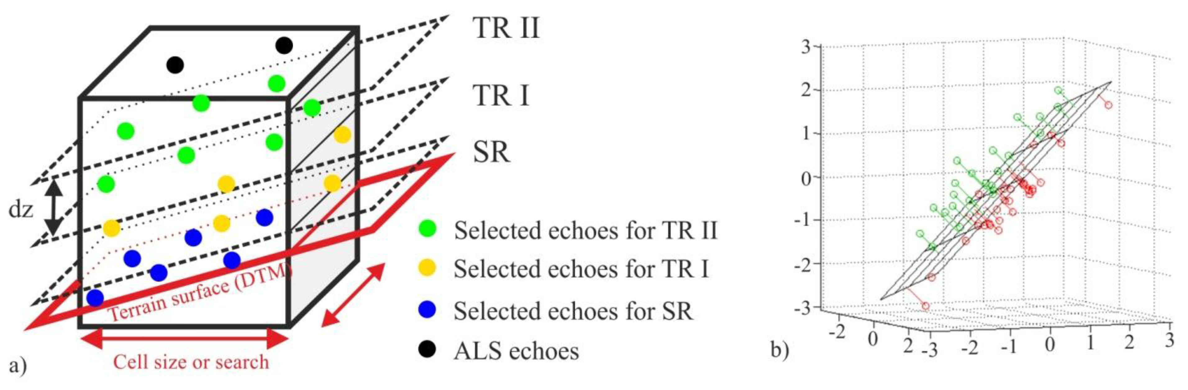
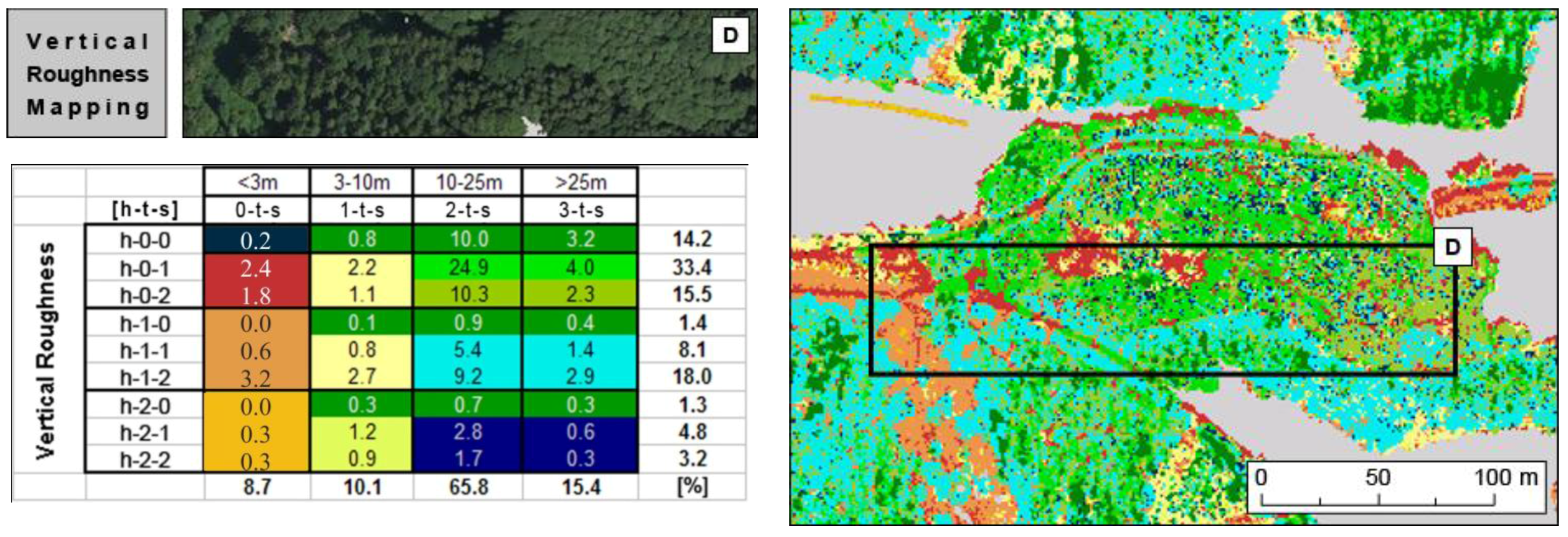
3.3. Vertical Roughness Mapping

After computing the ALS point cloud based roughness raster layers, as described above, they were jointly analyzed and combined, whereas a novel roughness classification scheme was developed, further referred to as ‘vertical roughness’. This roughness mapping concept incorporates information from various vegetation height layers using the capability of FWF-ALS, i.e., recording the entire backscatter spectrum from treetop to ground. Thus, it does not only give an indication of surface roughness patterns (limited to a very small height threshold above ground), but also includes information on the spatial distribution of brushwood (such as bushes and shrubs) and understory vegetation (up to 3.0 m).

The following paragraphs describe the advanced classification and analysis of the ALS-derived roughness raster products for the test site Bucklige Welt. First, SR and TR layers were jointly analyzed with regard to identification of significant spatial patterns with similar roughness characteristics. Adding yet another dimension to this integrated classification process—vegetation height as illustrated by a nDSM—rounds off a novel approach of mapping roughness in wooded areas on multiple vertical levels, from now on called ‘vertical roughness mapping (VRM)’. According to the basic objective of distinguishing smooth and rough surfaces, the SR raster was binary recoded (SR_bin → s) with the threshold defined at SR = 0.05 m plus one additional ‘no data’ category (s = 0). Grid cells featuring SR values larger than 0.05 m were thus considered rough (s = 2), while all records below that threshold were considered smooth (s = 1).

Regarding the structural undergrowth information inherent in the two TR raster layers a slightly different, but yet binary classification approach was chosen (TR_bin → t). One class of pixels (t = 1) depicts areas where echoes are recorded in both the lower vegetation layer TR I (very low brushwood or undergrowth up to 1.0 m, i.e., TR I: 0.2 ≤ d_z < 1.0 m) and the layer of understory vegetation up to 3.0 m TR II (i.e., TR II: 0.2 ≤ dz < 3.0 m). The second category (t = 2) includes regions where echoes were just recorded in the layer of TR II, but no recorded echoes exist in the lower layer of TR I (i.e., 0.2 ≤ d_z < 1.0). Again an additional class for ‘no data’ cells was appended (t = 0).

The combination of these binary SR and TR products with each layer featuring three value facets (1, 2, no data) resulted in a set of nine possible new classes (3 × 3 categories) describing different multi-level roughness characteristics.

In order to get an overall picture of the vertical vegetation structure, the nDSM was included as third input variable, i.e., height above terrain surface information classified in four forest layers (nDSM_4classes → h). Integrating this additional variable with four possible values results in 36 (3 × 3 × 4) classes eventually describing the full vertical vegetation structure. The 36 classes in the classification scheme and matrix described in Section 4.3. have to be interpreted as ‘h-t-s’ (h → nDSM_4classes, t → TR_bin, s → SR_bin). The first category (‘0-t-s’) is defined as ‘vegetation up to 3.0 m’ covering about 9% of the total area. As this class boundary coincides with the upper boundary of TR II, the nDSM integration does not expand the vertical roughness information content. The biggest part of the test site’s wooded area (65.8%) is however covered by trees which are between 10 m and 25 m high (category ‘2-t-s’). For validating the results of the ALS based vertical roughness mapping the in situ reference data (see Section 2.3) was used.

4. Results and Discussion

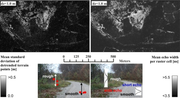
4.1. Surface Roughness (SR)

Figure 5 shows a derived SR raster layer for the test site Bucklige Welt featuring a terrain related variation of d_z < 0.2 m. All laser echoes within a 1.0 m neighborhood were considered in the plane fitting and standard deviation calculation process. The finally derived SR raster layer has a spatial resolution of 1.0 m. Distinguishing four classes based on natural groupings inherent in the data (‘natural breaks’ defined in the histogram) gives a good first impression of regional surface roughness variations in the study area. More than 50% of the total forested area is thus classified as having a very smooth surface (red, yellow) and around 25% show slightly higher deviations (green, blue). White pixels display ‘no data’ areas, i.e., areas where no laser echoes are available for the height layer of d_z < 0.2 m. Typically these areas are covered by very dense forest canopy preventing the laser beam from reaching the ground.

The detail image displayed in Figure 5 is the result of applying a focal neighborhood function (‘focal mean’, i.e., averaging within a circular neighborhood with a radius of 10 m) to the SR raster. For the displayed SR raster the option of ignoring ‘no data’ values in the calculation was chosen. With just around 15% of the pixels in forested areas featuring ‘no data’ values, it was decided to accept uncertainties entailed by ignoring those pixels and looking rather at the resulting generalized regional spatial patterns.

It becomes clear that in the northern woods of the study area very smooth surfaces prevail, while in the more heterogeneous southern parts surface in general tends to be rougher.

Figure 5. Surface roughness raster layer (1.0 m resolution) for the test site Bucklige Welt, classified in four roughness categories from smooth (red) to rough (blue). Non-wooded areas are masked out (in light yellow). Detail: Smoothed visual impression through applying a focal mean operator.

Figure 5. Surface roughness raster layer (1.0 m resolution) for the test site Bucklige Welt, classified in four roughness categories from smooth (red) to rough (blue). Non-wooded areas are masked out (in light yellow). Detail: Smoothed visual impression through applying a focal mean operator.

For the test site Wienerwald, Figure 6 shows on the left (1) the standard deviation of the detrended terrain echoes, and on the right (2) the mean echo widths using all selected terrain and near terrain echoes. High standard derivation (bright areas) indicates a high surface roughness. Large echo widths (bright areas) are caused by a certain vertical distribution of scatterers within a laser footprint and hence large echo widths indicate high surface roughness. The visual comparison of the derived roughness layers derived from the SR definitions, clearly shows similar spatial patterns of areas with high values of surface roughness (Figure 6). It can also be shown that this similarity is apparent for all applied height thresholds. The highest correlation coefficients (R = 0.62–0.63) between the two SR parameterizations are available for the roughness layers derived from echoes with heights (d_z) less than 0.25 m and 0.50 m, respectively. The linear regression between the standard deviation of the plane fitting residuals of terrain echoes and the mean echo widths derived from extended targets only show a slight decrease of the correlation coefficients, e.g., for echoes with d_z < 0.5 m from R = 0.63 to R = 0.58. This indicates that varying footprint sizes of single and multiple echoes have a negligible influence on the surface roughness parameterization. For the young forest subarea (see Figure 2, region 3) the correlation coefficient increases, e.g., to 0.68 for echoes with d_z < 0.25 m. For all other subareas (see Figure 2, region 1, 2, 4) the correlation coefficients decrease. Because a decrease was not expected, further statistics were calculated. For the grassland subarea, the standard deviation of the mean echo width is 0.03 ns and for the old forest stand subarea the standard deviation is 0.02 ns. Also the standard deviations of the mean standard deviation per raster cell of detrended terrain echoes are small and are in the range of 0.4 to 1.9 centimeters. This means that there is only a constant shift between the two roughness layers. Furthermore, this indicates very homogeneous and smooth surfaces, which corresponds to the information derived during the field check. Moreover, these small standard deviations can be interpreted as measurement noise from the FWF-ALS system used.

With such systems it is possible to acquire a sufficient amount of elevation measurements of the forest terrain surface even in very dense forest areas. As shown in Figure 7, areas indicated by high roughness values are mainly covered by low vegetation (e.g., bushes) or exhibit a very dense distribution of tree stems, which also account for terrain roughness as defined in this study. High roughness values are also available at the borders of forest roads and tracks where discontinuities (e.g., breaklines) commonly exist.

Figure 6. Surface roughness raster layer (1.0 m horizontal resolution) for the test site Wienerwald derived from FWF-ALS data. Left: Mean standard deviation per raster cell of detrended terrain and near terrain echoes for different height thresholds. Right: Mean echo width per raster cell calculated from terrain and near terrain echoes, respectively.

Figure 6. Surface roughness raster layer (1.0 m horizontal resolution) for the test site Wienerwald derived from FWF-ALS data. Left: Mean standard deviation per raster cell of detrended terrain and near terrain echoes for different height thresholds. Right: Mean echo width per raster cell calculated from terrain and near terrain echoes, respectively.

The majority of results indicate that FWF-ALS echo width information enables identifying areas with high terrain roughness without the need of a highly detailed geometrical representation of the ground surface (i.e., very dense point clouds).

However, there are still some uncertainties related to the use of the echo width for surface roughness parameterization. While pulse width estimates are relatively stable at high amplitudes, there is significant scattering at low amplitudes [28,30,31]. This needs to be taken into account in future studies. Furthermore, the comparison of the derived roughness layers has shown that small (i.e., in relation to the footprint size) terrain surface discontinuities, i.e., breaklines which are not covered by vegetation or stems lying on the terrain, are better represented in the geometry-based roughness layer than in the mean echo width approach (Figure 8). This can either be explained by the small laser footprints or by the fact that an object can only be covered partly by the laser footprint, and therefore, only minor vertical variations are available within the illuminated area.

Figure 7. Shading of the standard deviation of the detrended terrain echoes (d_z < 1.0 m) overlaid with pictures from different features.

Figure 7. Shading of the standard deviation of the detrended terrain echoes (d_z < 1.0 m) overlaid with pictures from different features.

Figure 8. Shading of the geometry-based roughness (left) and of the mean echo widths (right); d_z < 0.5 m. Black areas are ‘no data’ raster cells.

Figure 8. Shading of the geometry-based roughness (left) and of the mean echo widths (right); d_z < 0.5 m. Black areas are ‘no data’ raster cells.

4.2. Terrain Roughness (TR)

For the test site Bucklige Welt, the derived terrain roughness images TR I and TR II are shown in Figure 9. It can be seen that the two TR images, which are representative of two different height layers, contain much more ‘no data’ values than the previously described SR parameter (>70% for TR I, >60% for TR II compared to ~15% for SR).

Figure 9. Terrain roughness: (a) TR I and (b) TR II for the test site Bucklige Welt.

Figure 9. Terrain roughness: (a) TR I and (b) TR II for the test site Bucklige Welt.

Besides the same potential causes mentioned above, being (1) data errors or (2) very dense tree crowns preventing the laser beam reaching the analyzed height layer, no information in the ALS data can also signify open space without vegetation cover in reality. So, in fact even ‘no data’ values can provide valuable information in that context. Looking at the study site overview (top images in Figure 9) it is apparent that there is more TR data recorded in the southern parts of the study site. Anyhow, at this level of detail also in those areas just very little variation is detected in TR I. Values in TR II show a slightly different picture, with (1) featuring a somewhat higher information density (i.e., 37% vs. 27% for TR I) and (2) featuring more variation (i.e., mean value of 0.22 vs. 0.05 in TR I). The latter is also related to the larger vertical focus of this specific parameter (0.2 < d_z < 3.0). Looking at the TR raster layers in more detail (details in Figure 9), local fine-scale roughness variations become visible. The spatial distribution of available information is very similar. The slightly higher data density in TR II can indicate: (1) very dense vegetation in this forest layer, again preventing the laser beam from reaching lower layers; or (2) higher vegetation with branches starting somewhere around eye level, but not having any undergrowth beneath.

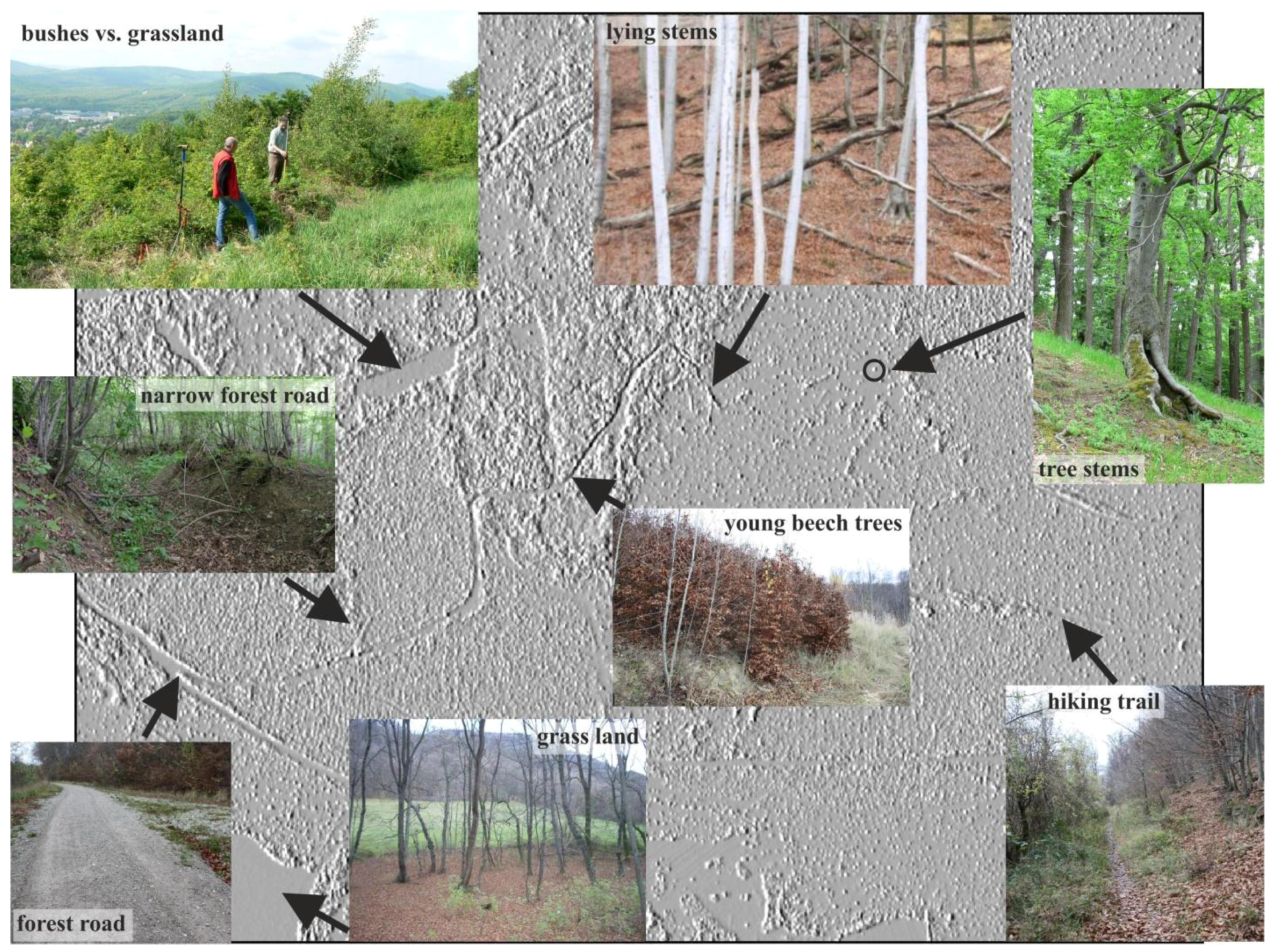
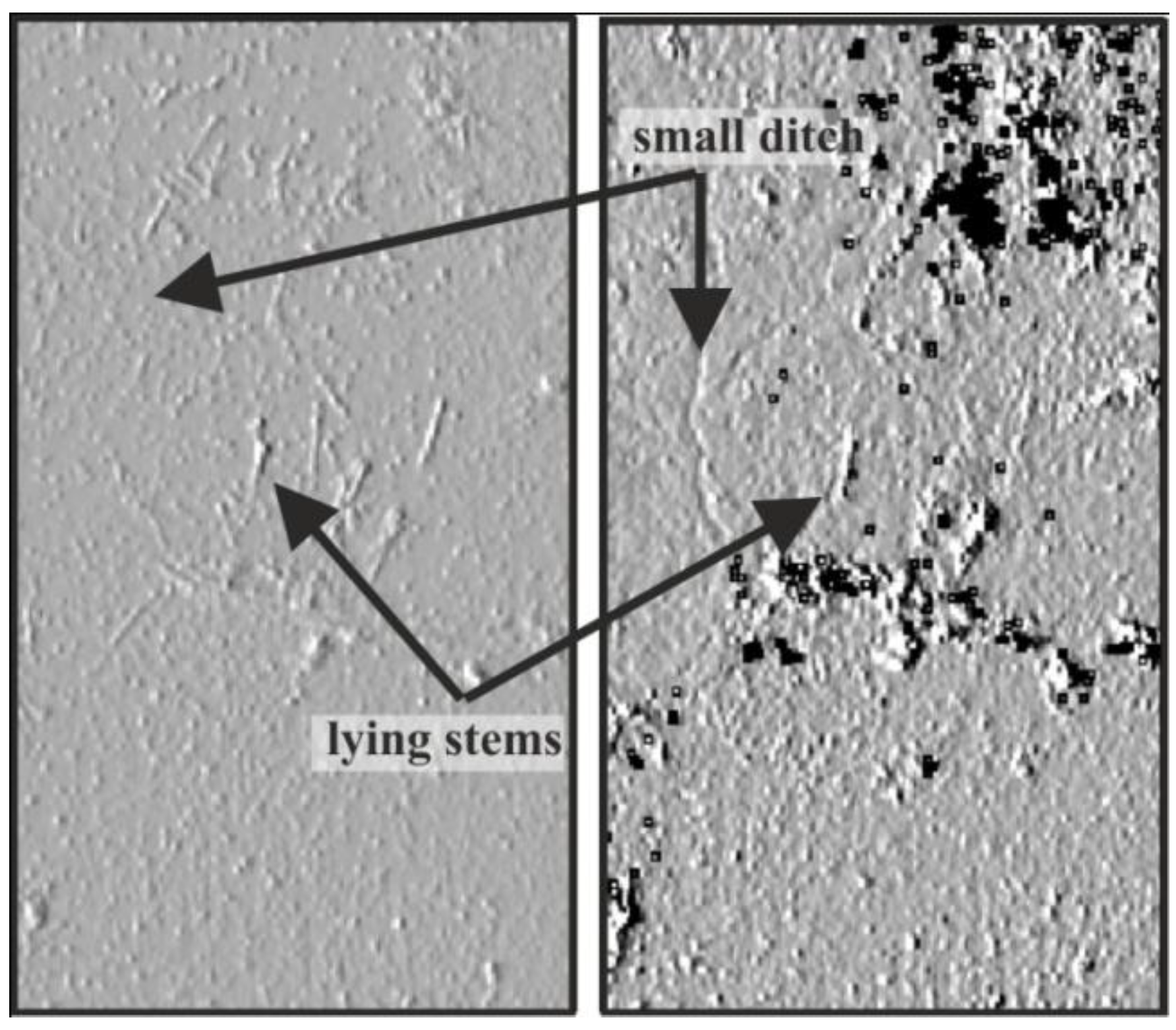
4.3. Vertical Roughness Mapping

For the test site Bucklige Welt, most frequent classes considering the vertical roughness mapping classification scheme are the categories with t = 0 (h-0-s), i.e., having no TR data records, with 0-1 particularly standing out. This class covering about one third of the study area (33.4%) delineates areas with smooth surface and no recorded echoes in both layers of understory vegetation (TR I: 0.2 m ≤ d_z < 1.0 m, and TR II: 0.2 m ≤ d_z < 3.0 m). In fact five classes out of the 36 categories stand out, each featuring more than 5% and in total covering about 60% of the test site. 22 of the remaining classes only account for less than 2% each. The, by far, most dominant class (24.9%) is ‘2-0-1’ (light green in Figure 10) featuring an overall height of between 10 m and 25 m, smooth surface, and no echo records regarding undergrowth.

Figure 10. Vertical roughness map and classification scheme for a detailed area of the test site Bucklige Welt, and aerial image for comparison (D).

Figure 10. Vertical roughness map and classification scheme for a detailed area of the test site Bucklige Welt, and aerial image for comparison (D).

In general, nearly 65% of the total forest area shows no backscatter records in the mid-vegetation layer (i.e., the ‘h-0-s’ category group). In that case some kind of undergrowth is present, most of the times it spans both the whole vertical range between 0.2 m and 3.0 m above ground (t = 1, i.e., echoes recorded in both TR I and TR II) and ‘rough’ surface conditions (s = 2) → ‘h-1-2’ pixels summing up to 18%. When looking at the ‘h-1-s’ type, thus ignoring surface roughness variation, these regions even cover 27.5% of the total study area. Classes with TR information exclusively recorded in the higher level of understory vegetation between 1.0 m and 3.0 m (t = 2, i.e., the ‘h-2-s’ category) occur only very sparsely covering a total of less than 10% of the study area. Pixels assigned to these classes can mainly be attributed to large trees with branches reaching down to the 3.0 m range but not all the way down to the ground.

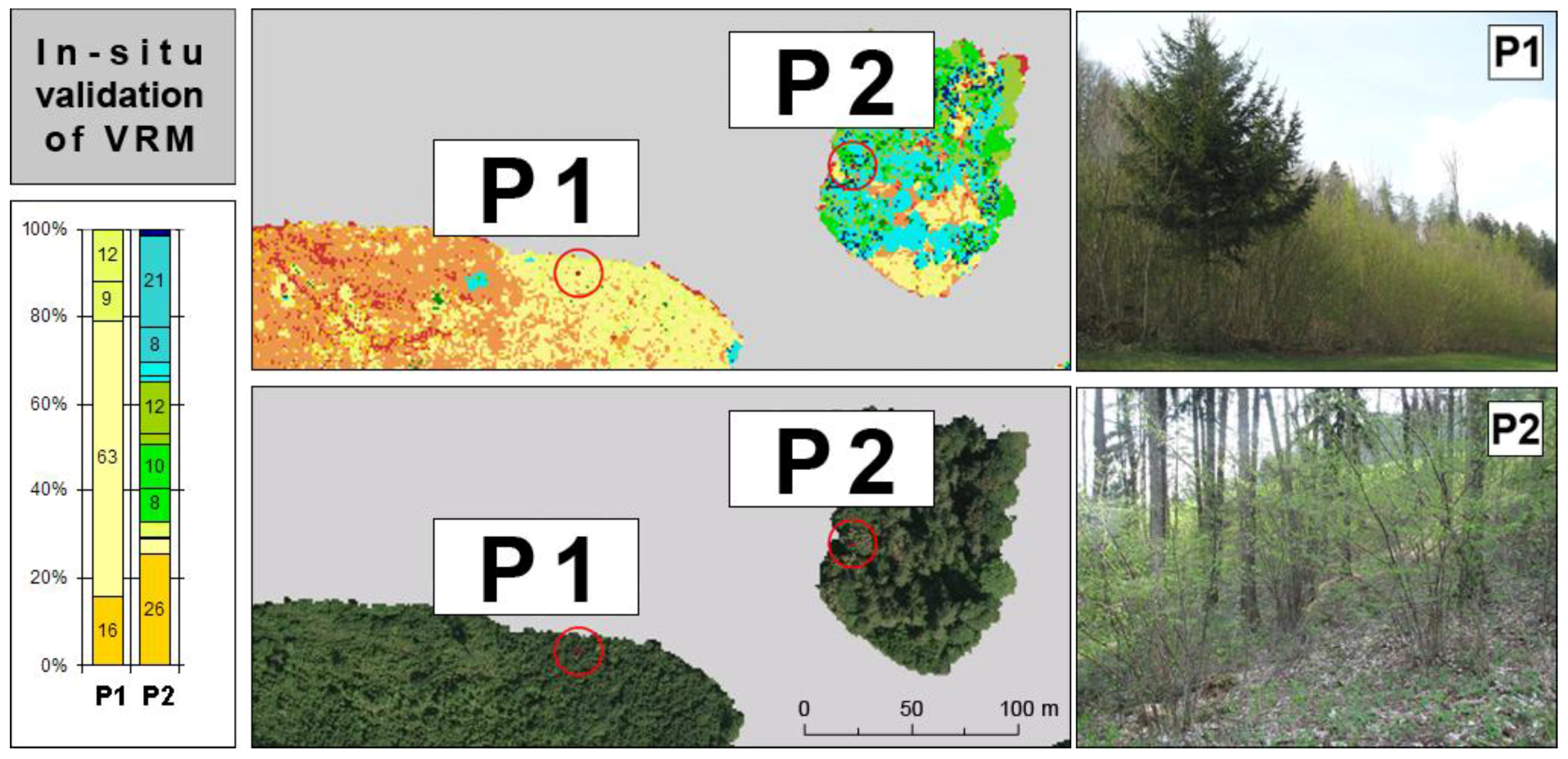
4.5. Validation of the Vertical Roughness Map

For the test site Bucklige Welt, two selected reference points of varying characteristics will be presented in detail, serving as examples for cross-validating ALS derived roughness and reality conditions. Figure 11 shows the VRM for the examined area with the aerial image included for comparison and orientation reasons.

Figure 11. In situ validation of VRM for a detail of the test site Bucklige Welt.

Figure 11. In situ validation of VRM for a detail of the test site Bucklige Welt.

For each of the two reference points (P1, P2), a vertical-bar graph is presented illustrating the VRM pattern (class ratios) within a 10 m neighborhood (marked with red circles in the map). To illustrate reality conditions, pictures from the field survey are shown in the bottom part of Figure 11. First, spatial roughness patterns as illustrated in the raster map and class ratio numbers are analyzed. For reference point P1, a good portion of its immediate neighborhood (63%) is classified as ‘1-1-2’ (light yellow in Figure 11), i.e., overall rather low vegetation height <10 m (h = 1), recorded echoes in both terrain layers TR I and TR II (t = 1), along with ‘rough surface’ (s = 2). With respect to the entire study area, this is a very untypical picture with ‘1-1-2’ just covering less than 3% in total. These ALS-based ratio values shown in the vertical-bar graph are confirmed by looking at the collected reference data, with photo P1 showing dense low-level deciduous vegetation with branches and leaves throughout the vertical range. Also in an additionally available reference data set (provided by the Research and Training Centre for Forests, Natural Hazards and Landscape, BFW) this region is qualitatively described as ‘young and very dense deciduous forest including undergrowth’. 21% are classified as ‘1-2-s’ (light green) while the remaining 16% are assigned to ‘0-2-s’ (orange), i.e., no recorded echoes in TR I (t = 2) at slightly varying overall tree height (h = 0 or 1). As surface information is available anyhow (either smooth or rough), it is unlikely that too dense top-level vegetation prevented the laser beam from ‘seeing’ the lower level. As during the field campaign indeed some parts of this specific forest patch were observed not featuring any low-level brushwood the classified VRM information is expected to be correct and significant. Reference point P2 shows a completely different picture. Photo P2 in Figure 11 displays mixed and rather loose vegetation including for example, large coniferous trees, small broadleaf bushes and leaf-covered surface.

This is confirmed and even emphasized by the ALS based VRM. Looking at the class ratio values shown in the vertical-bar graph and at the raster layer, no predominant category can be detected, but rather a heterogeneous mix of various roughness classes in the immediate neighborhood of the reference point. From bare soil (‘0-0-1’) to the largest trees (3-t-s) the entire range of roughness categories is present. Photo documentation not necessarily delivers representative results, also because of possible varying characteristics around the view point. However, during data collection attention was paid to that issue. As the field survey was carried out about two years after the ALS data had been recorded, data mismatches can be due to the different acquisition dates. Summing it up, results are very encouraging and it seems that advanced vertical roughness mapping is possible at a certain spatial level of detail based on ALS information.

5. Conclusions

In addition to the 3D coordinates, FWF-ALS delivers laser point attributes (e.g., signal amplitude, echo width) providing further quantities to characterize surface properties. The presented analyses have shown that the FWF-ALS echo width derived surface roughness layer, indicates areas with high roughness similarly to the geometric definition requiring very high laser point densities. The analyses have further shown that the echo width can be used as a surface roughness parameter even with low terrain point densities compared to the geometry-based computation.

Furthermore, a novel approach of data classification and revaluation was presented with the focus on identifying ‘roughness’ on various vertical layers in forested areas. Previously calculated roughness raster layers were jointly analyzed in order to develop a novel roughness classification scheme considering the entire vertical structure of vegetation from surface to treetop. This classification procedure is introduced as vertical roughness mapping (VRM). Results of the roughness classification were cross-validated against collected in situ reference data indicating a high level of thematic accuracy. As follow-on analysis, several ways of smoothing the VRM raster files (i.e., information-preserving ‘intelligent’ generalization) will be tested in order to derive areal roughness hot spots useful for terrain related hazard assessments (e.g., water hazards, mass movements).

In future research, the influence of varying flying heights and incidence angles on the echo width will be investigated. Furthermore, the increasing uncertainty of the echo width with weak signals, resulting in low amplitudes, will be studied.

References

1. Margreth, S.; Funk, M. Hazard mapping for ice and combined snow/ice avalanches—Two case studies from the Swiss and Italian Alps. Cold Regions Sci. Technol. 1999, 30, 159–173. [Google Scholar] [CrossRef]
2. Dorren, L.K.A.; Heuvelink, G.B.M. Effect of support size on the accuracy of a distributed rockfall model. Int. J. Geogr. Inf. Sci. 2004, 18, 595–609. [Google Scholar] [CrossRef]
3. Govers, G.; Takken, I.; Helming, K. Soil roughness and overland flow. Agronomie 2000, 20, 131–146. [Google Scholar] [CrossRef]
4. Gómez, J.A.; Nearing, M.A. Runoff and sediment losses from rough and smooth soil surfaces in a laboratory experiment. Catena 2005, 59, 253–266. [Google Scholar] [CrossRef]
5. Jutzi, B.; Stilla, U. Waveform Processing of Laser Pulses for Reconstruction of Surfaces in Urban Areas. In Proceedings of 3th International Symposium: Remote Sensing and Data Fusion over Urban Areas, URBAN 2005, Tempe, AZ, USA, 14–16 March 2005; Volume 36, Part 8 W27. p. 6.
6. Ghinoi, A.; Chung, C.-J. STARTER: A statistical GIS-based model for the prediction of snow avalanche susceptibility using terrain features—Application to Alta Val Badia, Italian Dolomites. Geomorphology 2005, 66, 305–325. [Google Scholar] [CrossRef]
7. McClung, D.M. Characteristics of terrain, snow supply and forest cover for avalanche initiation caused by logging. Ann. Glaciol. 2001, 32, 223–229. [Google Scholar] [CrossRef]
8. Margreth, S. Lawinenverbau im Anbruchgebiet; Bundesamt für Umwelt BAFU, WSL Eidgenössisches Institut für Schnee- und Lawinenforschung SLF: Bern, Germany, 2007. [Google Scholar]
9. Höller, P.; Fromm, R.; Leitinger, G. Snow forces on forest plants due to creep and glide. Forest Ecol. Manag. 2009, 257, 546–552. [Google Scholar] [CrossRef]
10. Lavee, H.; Kutiel, P.; Segev, M.; Benyamini, Y. Effect of surface roughness on runoff and erosion in a Mediterranean ecosystem: the role of fire. Geomorphology 1995, 11, 227–234. [Google Scholar] [CrossRef]
11. Rai, R.K.; Upadhyay, A.; Singh, V.P. Effect of variable roughness on runoff. J. Hydrol. 2010, 382, 115–127. [Google Scholar] [CrossRef]
12. Markart, G.; Kohl, B.; Sotier, B.; Schauer, T.; Bunza, G.; Stern, R. Provisorische Geländeanleitung zur Abschätzung des Oberflächenabflussbeiwertes auf alpinen Boden-/Vegetationseinheiten bei konvektiven Starkregen (Version 1.0). BFW-Dokumentation. 2004, 3, 83. [Google Scholar]
13. Cord, A.M.; Baratoux, D.; Mangold, N.; Martin, P.D.; Pinet, P.C.; Costard, F.; Masson, P.; Foing, B.; Neukum, G. Surface roughness and geological mapping at sub-hectometer scale from the High Resolution Stereo Camera onboard Mars Express. Icarus 2007, 191, 38–51. [Google Scholar] [CrossRef]
14. Jester, W.; Klik, A. Soil surface roughness measurement—Methods, applicability, and surface representation. Catena 2005, 64, 174–192. [Google Scholar] [CrossRef]
15. Smith, M.J.; Asal, F.F.F.; Priestnall, G. The Use of Photogrammetry and LIDAR for Landscape Roughness Estimation in Hydrodynamic Studies. In Proceedings of International Society for Photogrammetry and Remote Sensing XXth Congress, Istanbul, Turkey, 12–23 July 2004; Volume XXXV, WG III/8. p. 6.
16. Straatsma, M.W.; Baptist, M.J. Floodplain roughness parameterization using airborne laser scanning and spectral remote sensing. Remote Sens. Environ. 2008, 112, 1062–1080. [Google Scholar] [CrossRef]
17. Aubrecht, C.; Höfle, B.; Hollaus, M.; Köstl, M.; Steinnocher, K.; Wagner, W. Vertical Roughness Mapping—ALS Based Classification of the Vertical Vegetation Structure in Forested Areas. In Proceedings of ISPRS TC VII Symposium: 100 Years ISPRS, Vienna, Austria, 5–7 July 2010; Volume XXXVIII, Part 7B. pp. 35–40.
18. Hollaus, M.; Höfle, B. Terrain Roughness Parameters from Full-Waveform Airborne LiDAR Data. In Proceedings of ISPRS TC VII Symposium: 100 Years ISPRS, Vienna, Austria, 5–7 July 2010; Volume XXXVIII, Part 7B. pp. 287–292.
19. Wagner, W.; Ullrich, A.; Melzer, T.; Briese, C.; Kraus, K. From Single-Pulse to Full-Waveform Airborne Laser Scanners: Potential and Practical Challenges. In Proceedings of International Society for Photogrammetry and Remote Sensing XXth Congress, Istanbul, Turkey, 12–23 July 2004; Volume XXXV, Part B/3. p. 6.
20. Hollaus, M.; Mücke, W.; Höfle, B.; Dorigo, W.; Pfeifer, N.; Wagner, W.; Bauerhansl, C.; Regner, B. Tree Species Classification Based on Full-Waveform Airborne Laser Scanning Data. In Proceedings of 9th International Silvilaser Conference, College Station, TX, USA, 14–16 October 2009; pp. 54–62.
21. SCOP++—Programpackage for Digital Terrain Models. Tuwien: Vienna, Austria; Available online: http://www.inpho.de (accessed on 1 June 2010).
22. Hollaus, M.; Mandlburger, G.; Pfeifer, N.; Mücke, W. Land Cover Dependent Derivation of Digital Surface Models from Airborne Laser Scanning Data. In Proceedings of ISPRS Technical Commission III Symposium: Photogrammetric Computer Vision and Image Analysis, Paris, France, 1–3 September 2010; Volume 39, p. 6.
23. OPALS—Orientation and Processing of Airborne Laser Scanning Data. Tuwien: Vienna, Austria. Available online: http://www.ipf.tuwien.ac.at/opals/ (accessed 1 June 2010).
24. Kraus, K. Photogrammetry: Geometry from Images and Laser Scans, 2nd ed; Walter de Gruyter: Berlin, Germany, 2007; p. 459. [Google Scholar]
25. Höfle, B.; Pfeifer, N. Correction of laser scanning intensity data: Data and model-driven approaches. ISPRS J. Photogramm. Remote Sens. 2007, 62, 415–433. [Google Scholar] [CrossRef]
26. Höfle, B. Detection and Utilization of the Information Potential of Airborne Laser Scanning Point Cloud and Intensity Data by Developing a Management and Analysis System. Ph.D. Thesis, Faculty of Geo- and Atmospheric Sciences, University of Innsbruck, Innsbruck, Austria, 2007. [Google Scholar]
27. Geist, T.; Höfle, B.; Rutzinger, M.; Pfeifer, N.; Stötter, J. Laser scanning—A paradigm change in topographic data acquisition for natural hazard management. In Sustainable Natural Hazard Management in Alpine Environments; Veulliet, E., Stötter, J., Weck-Hannemann, H., Eds.; Springer: Berlin, Germany, 2009; pp. 309–344. [Google Scholar]
28. Wagner, W.; Ullrich, A.; Ducic, V.; Melzer, T.; Studnicka, N. Gaussian decomposition and calibration of a novel small-footprint full-waveform digitising airborne laser scanner. ISPRS J. Photogramm. Remote Sens. 2006, 60, 100–112. [Google Scholar] [CrossRef]
29. Doneus, M.; Briese, C.; Fera, M.; Janner, M. Archaeological prospection of forested areas using full-waveform airborne laser scanning. J. Archaeol. Sci. 2008, 35, 882–893. [Google Scholar] [CrossRef]
30. Lin, Y.; Mills, J. Factors influencing pulse width of small footprint, full waveform airborne laser scanning data. Photogramm. Eng. Remote Sensing 2010, 76, 49–59. [Google Scholar] [CrossRef]
31. Mücke, W. Analysis of Full-Waveform Airborne Laser Scanning Data for the Improvement of DTM Generation. M.Sc. Thesis, Institute of Photogrammetry and Remote Sensing, Vienna University of Technology, Vienna, Austria, 2008; p. 67. [Google Scholar]