1. Introduction
With the rapid worldwide increase in demand for palm oil and lumber, Borneo’s rain forests are under heavy deforestation pressure [
1,
2]. The rate at which forests are being cut down [
3] is such that policymakers at all levels are actively seeking solutions with a variety of approaches to the impending losses of this vital resource [
4,
5,
6,
7]. The consequences of the extensive deforestation of Borneo are felt both at the local and global scale, and it is essential to acknowledge and understand the phenomenon through frequent and efficient monitoring.
The vast expanse of Borneo, the third largest island of the world, and the inaccessibility of many of its regions make remote sensing one of the few viable options for monitoring deforestation for the whole island. However, abundant year-round cloud cover presents a considerable challenge to remote sensing programs [
4]. Large parts of a typical single remotely sensed image of the island are completely obscured by clouds. No single period of the year stands out as optimal for image acquisition: the island is one of the wettest parts of the world and it rains throughout the year. Although cloudiness diminishes in the drier months of May, June and July, fire-aided land clearing emits large amounts of haze creating atmospheric contaminants during that time [
5,
6]. These complicate assessments and need to be taken into account in studies of Borneo using remotely sensed data.
We have developed strategies for employing high-resolution Google Earth [
8] images as validation data, using them to construct a spatially explicit training and testing database for Moderate-Resolution Imaging Spectroradiometer (MODIS) image classification. Although relatively rare in Borneo, the coverage of high-resolution Google Earth images is rapidly increasing. Unlike daily MODIS data, those images are mostly cloud free and of a resolution high enough to very easily distinguish land covers and land uses of many types. Yet because the images are captured at a wide variety of dates in this region, their use for validation data is not straightforward.
Using MODIS and Google Earth data, we have produced a time series of nine maps showing likely deforestation. Each of the maps represents hotspots for an entire year, between year 2000 and 2009. The methodology employed to produce this time series demonstrates techniques that can be used to circumvent the obstacles that typically hinder systematic remote sensing in Borneo and other heavily clouded areas.
2. Methods
2.1. MODIS Data and Annual Composites
The problem of persistent cloud coverage in remotely sensed images can be overcome by using image compositing techniques [
7,
9], and such techniques have been used in the past to obtain suitable coverage of Borneo [
6,
10,
11]. Since Borneo is highly affected by cloud cover, we needed a very high redundancy in our images as well as an extended compositing period.
Images acquired by the Terra satellite with the MODIS instrument were our deforestation detection data source. For this work, MODIS-Terra presents several useful characteristics. Firstly, Terra acquires almost-global daily coverage of the Earth’s surface and it has done so since early 2000 [
12]. Second, Terra passes over Borneo in the morning, when fewer clouds are present than in the afternoon [
13]. Third, key vegetation indices are systematically developed to produce relatively cloud-free, atmospherically corrected, and nadir-adjusted vegetation maps [
14,
15]. As a result, no additional calibration is needed prior to the compositing of the images. Finally, MODIS data is distributed in a variety of data products with per-pixel quality assessment flags. In our case, we use the Vegetation Indices 16-Day L3 Global 250 m datasets (short name MOD13Q1).
To detect changes in land cover from year to year, we used the Enhanced Vegetation Index (EVI) [
13] a vegetation index optimized for the enhanced capabilities offered by the MODIS sensor. Compared to other well-known indices like NDVI, EVI is less prone to saturation in high biomass environments such as rain forests, and is particularly resilient to variation in illumination and atmospheric composition [
13,
15]. The MOD13Q1 dataset that contains the EVI data is intended for the study of vegetation and is comprised of twelve data layers that have a spatial resolution of 250 m. Also included in the dataset is a metadata layer giving a per-pixel detailed quality assessment of the vegetation index [
13].
When producing a single MOD13Q1 dataset, the MODIS compositing algorithm picks the best pixels from sixteen days of images in order to reduce the amount of pixels that are partially or completely obscured by clouds, cloud shadows or other atmospheric contaminants [
13]. However, due to the exceptionally persistent cloud cover over Borneo, a sixteen-day period is insufficient to produce obstruction-free images. This motivated us to create annual composite images formed from a full year of MOD13Q1 16-day composites. We were able to assemble images taken throughout the year since Borneo’s forests are evergreen and receive precipitation year-round. As a result, intra-annual variation in phenology and spectral variation in vegetation indices throughout the year over most of the forest cover is relatively minor [
4]. Furthermore, the mean compositing method used here minimizes the impact of reflectance variations that, although small, are still present [
9,
11].
To properly implement the mean compositing method, we made sure to remove all pixels in the source images whose quality could be overly affected by atmospheric contaminants. We used the detailed quality assessment data layer to identify the highest-quality usable pixels with which to form the annual composite. We assembled our annual images using only pixels with a quality level of at least 11 out of 13, the highest possible quality level. This quality screening retained about 30% of the highest-quality composite pixels in a given 16-day image, and avoided visible artifacts in yearly assembled images when this strict criterion was not used. Pixels with quality values lower than 11 often displayed visual evidence of atmospheric contamination and cloud shadows.
Once composited, a full year of imagery gives an almost complete image of the island. Individual yearly composites covered between 96.2% and 98.7% of the island. A small percentage of the island remained unfilled in each year because, even after compositing a full year of MODIS imagery, we could not find any source images in which those blank areas were not overly affected by cloudiness. Therefore, our assembled images must be considered more like an exhaustive sampling than a true wall-to-wall census of the island’s surface. The resulting images span a decade, from early 2000 until the end of 2009. Consequently, the composited EVI images were employed for detection of deforestation hotspots.
2.2. Image Differencing
We used simple image differencing, one of the most common methods of change detection [
16], to identify major changes in surface reflectance that were likely due to deforestation. Because we are looking for drops in the EVI from one year to the next, we deliberately restricted that change detection to potential forest clearings. Ideally, the time span between the subtracted EVI images should be relatively short; otherwise the cleared areas that should have been detected might have become revegetated, either through human intervention or through forest regrowth, which can be considerable [
17]. The resulting increase of the EVI value would therefore have hindered our ability to effectively detect the clearings. For this reason, we could not use our method solely with a composite image for 2000 and another one for 2009 because a lot of deforestation events would have gone unnoticed. Consequently, we implemented our method by subtracting a composited image of a given year from the composited image of the subsequent year to produce a chronological series representing the annual changes in EVI values from the year 2000 through the year 2009. Negative values in this series of nine images represent drops in EVI values that correspond to a loss of vegetative cover. It is the substantial drops in EVI we aimed to detect in order to identify pixels where deforestation happened from one year to the next.
2.3. Creating a Google Earth Ground-Truth Database
High-resolution data from Google Earth is a relatively untapped new source of validation data for remote sensing studies [
18,
19]. The spatial resolution of the images is high enough to allow clear visual interpretation of the land cover. As such, they can be used as training and validation data to aid and evaluate classifications in coarser datasets. Yet the imagery is not available everywhere (
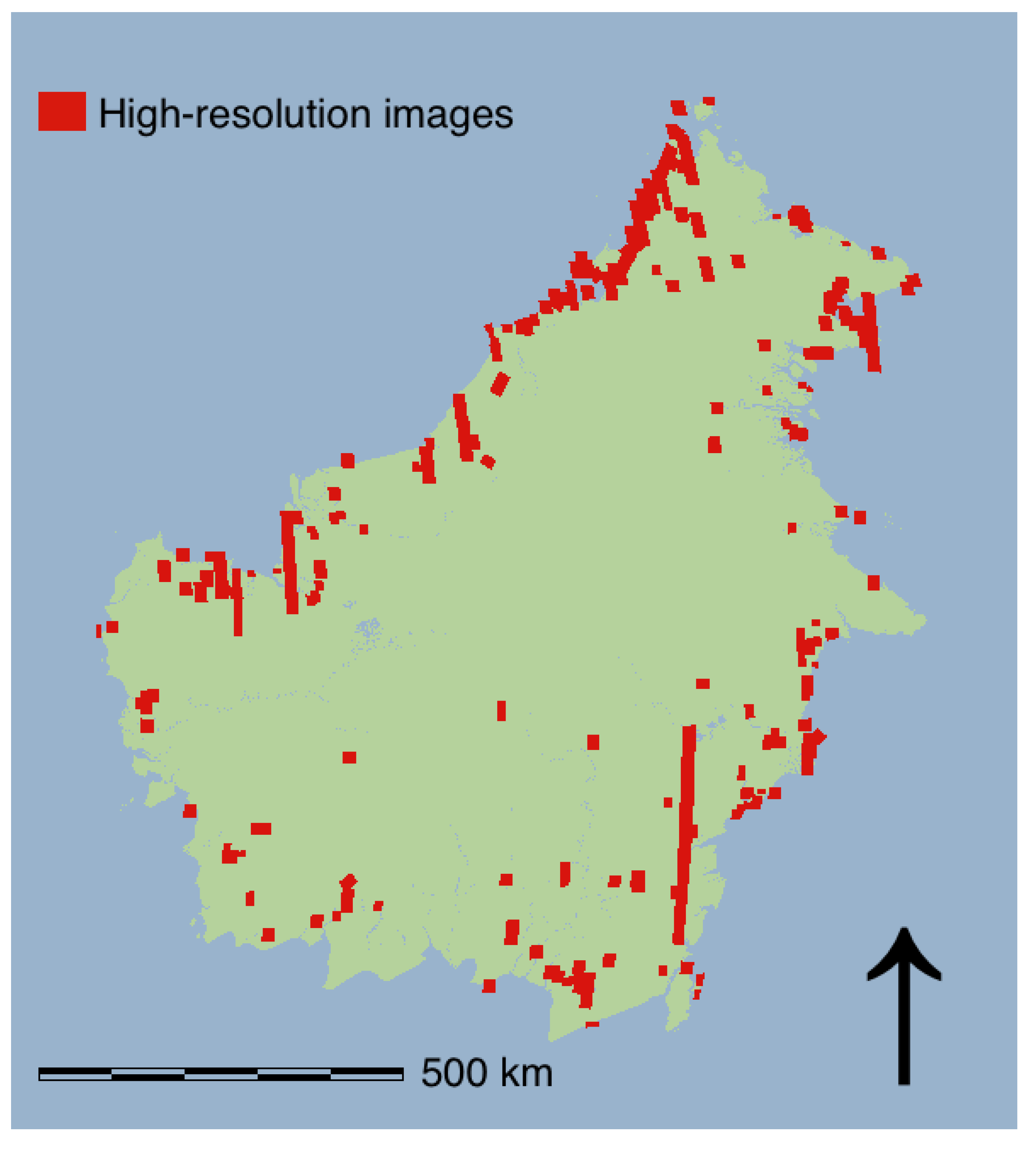
Figure 1) and can be captured at a wide variety of times in a given study period. At the present time, the database of available imagery in Google Earth in Borneo is mostly limited to a single snapshot in time, with very little repeat high-resolution imagery. Its use in a validation database is rewarding but requires carefully attention, as described below.
An initial step in the creation of the spatial database was to digitize, from within Google Earth, a polygon layer of the areas where high-resolution imagery is available for Borneo. We imported that vector layer in GRASS GIS [
20], the GIS we used to composite and differentiate the MODIS data, and converted it to a raster layer. We matched the resolution and projection of this raster layer to those of our MODIS images (
Figure 1). We generated 500 random raster points within the areas with high-resolution images. Each of these points corresponds to a pixel matching the 250 m resolution of the MODIS data. Because areas that had been deforested between 2000 and 2009 was a small percentage of the overall land area, we identified the subset of random points in which the largest drop of EVI during the period was among the 1% most extreme of all pixels. The training and testing data set were roughly balanced between purely random pixels and those pixels that were more likely to contain evidence of deforestation.
The random raster sample points were converted to polygons. Because of the resolution of the raster layer, each of the converted polygons has the same size and alignment as single pixels in the MODIS images. By linking this vector layer to an SQLite database, we produced a spatial database (
Table 1).
The spatial database was built in order to store validation data. To populate our database, we generated a KML file from our validation vector layer. We labelled the polygons in the KML file with the corresponding index numbers of the matching GRASS GIS vector layer. In Google Earth, we visually interpreted each of the validation polygons of the KML layer and we recorded the results in the SQLite database.
Figure 1.
Island of Borneo showing location of Google Earth high-resolution imagery from between 2000 and 2009.
Figure 1.
Island of Borneo showing location of Google Earth high-resolution imagery from between 2000 and 2009.
Table 1.
SQLite spatial database excerpt.
Table 1.
SQLite spatial database excerpt.
| Polygon ID | Type of event | Year |
|---|
| 1 | Non-change | 2002 |
| 2 | Change | 2005 |
| 3 | Non-change | 2002 |
| 4 | Discarded | |
| 5 | Non-change | 2008 |
| 6 | Change | 2004 |
| … | … | … |
2.4. Effects of Image Timing on Use of Google Earth Imagery for Ground Truthing
While navigating in Google Earth, the program displays the capture date of the imagery being shown. In addition, Google Earth version 5 introduced the ability to see a timeline of images in a given area, and move quickly between image dates [
21]. When using Google Earth imagery as a ground-truth indication of a deforestation event, this timeline presents considerable strengths: one can move through a timeline of imagery and quickly view the interval in which a major deforestation event happened. Yet the irregular intervals between images present considerable challenges as well. In effect, because coverage is irregular and infrequent, it is generally not possible to use these Google Earth high-resolution images to pinpoint exactly when a specific change event took place: if one image from mid-2002 shows an intact forest but the subsequent image shows a deforested landscape in mid-2005, when did the change occur? There are several potential reasonable answers, each of which could affect the validation dataset’s ability to be matched with the MODIS change image. With this in mind, we developed the following algorithm to populate the database. We interpreted the high-resolution Google Earth images delimited by the polygon samples of our validation layer and we recorded the results in the database. The characteristics and implication of this database are described in the Results section.
Figure 2 illustrates the step-by-step iterative process of interpreting the sampled polygons of validation data and the populating of the validation database:
In Google Earth, navigate to the sampled polygon. This polygon delimits a single pixel of the MODIS data grid.
Sometimes there is more than one high-resolution image available for a given area. A slider enables the verification of whether or not such is the case.
Decide whether the pixel can be interpreted. For this to be the case, it is necessary that either clear clues of recent deforestation are present, or that it is obvious land use has remained undisturbed since the beginning of the time series being produced (in our case the year 2000). Furthermore, if the area sampled is outside the scope of our study, such as a pixel over farmland or wetlands, note it for discard in step 7.
Check for clues of recent deforestation, such as bare lands or recently planted oil palm.
If the result of the sample interpretation (step 4) is that the sample has been subject to deforestation, it is noted in the spatial database. The year of the image acquisition is noted in the database as well.
Otherwise, if the result of the sample interpretation (step 4) is that the sample has not been subject to deforestation, it is noted in the spatial database. The year preceding the image acquisition is noted in the database as well.
If a pixel cannot be used, mark it as discarded in the validation database.
For Borneo, a few areas sampled have multiple high-resolution images available. In those cases, a slider in Google Earth enables one to view in succession each of these images. In such a situation, the first step is to check whether or not any of the high-resolution images can be interpreted using the criteria of step 3.
Check to see if any of the interpretable high-resolution images show clues of deforestation using the criteria of step 4.
If there is a change event present on one or some of the high-resolution images (corresponding to deforestation), select the oldest high-resolution image where traces of the change event can be seen for the interpretation of the sample. This oldest image is the nearest one in time to the effective time the event actually happened.
If no change can be detected on the high-resolution images, choose the high-resolution image that is the newest one for interpretation, as it will validate the absence of change for a longer period.
Continue to the next sampled pixel for interpretation.
Figure 2.
Validation sample interpretation and validation database building workflow.
Figure 2.
Validation sample interpretation and validation database building workflow.
2.5. Detecting an Optimal Threshold of Annual Difference in EVI
We used PEST software [
22] to determine the threshold indicating the level of change in EVI values that corresponded to a deforestation event. PEST is a black-box parameter estimation tool that accepts a model of any type with text input, output, and parameter files, and uses results from model runs to adjust parameter values, seeking an optimal fit with observations. As described above, the observed data used for validation is the spatial sampling database of Google Earth high-resolution images. The parameter of estimation was the EVI difference between MODIS composites that estimated that a land clearing had occurred in the interim. This EVI difference threshold was iteratively tested to find the best agreement among pixels of change and non-change in high-resolution Google Earth samples. Given that the EVI product is produced consistently from Level 3 MODIS data that has undergone calibration and atmospheric correction, it makes sense to determine a single detection threshold for all the year-to-year EVI difference images.
Figure 3.
Threshold determination workflow using the PEST software package.
Figure 3.
Threshold determination workflow using the PEST software package.
Figure 3 illustrates the steps by which PEST estimates the best possible detection threshold in the context of this study:
An initial detection threshold is fed into PEST for the first run of the model. This estimate should be reasonable but does not need to be particularly near the optimum value.
For a given threshold, PEST launches our model. Nine change / non-change maps showing potential hotspots are produced. These nine maps cannot be validated as is by PEST. To that end, we built our model so that a number of by-products are generated from those maps in steps 3 to 7.
A cumulative map of all the change detected between the year 2001 and the year 2006 is produced from the maps created in step 2. In this maps, one class represents areas where change was detected in at least one of the map produced in the previous step for the 2001 to 2006 period. The other class represents areas where change was never detected during that time.
As in step 3, a cumulative map of all the change detected is produced but from all the maps created in step 2.
Concordance between the non-change classes of the hotspots maps created in step 2 and the validation data is estimated. For each of the maps, the number of pixels of the non-change class that correspond to the samples of non-change in the validation database is computed. The maps have to match the sample data both in class (i.e., they must both be classified as non-change) and in time. For example, if the sample of a high-resolution image taken in 2005 is classified as non-change, hotspots maps for each of the years preceding 2005 should show no change at that location. Therefore, this sample would be used to check concordance of the 2001, 2002, 2003 and 2004 maps with the validation data.
The Kappa coefficient is estimated for each of the two classes of the map created in step 3. We chose to estimate concordance of both classes for the cumulative map up to the year 2006 because we had a fairly balanced number of samples for each of the classes (66 samples for the non-change class and 57 samples for the change class). The Kappa coefficient estimated here evaluates the concordance between our validation data and the change detection maps produced by PEST that might be the result of chance. As such, it is a complement to the per class concordance that is estimated in steps 5 and 7 which disregard chance.
The cumulative map of change produced in step 4 enabled us to check concordance between all the change events sampled in our validation data and all the change detected in the maps of step 2. Here, the number of pixels of the change class that correspond to the samples of change in the validation database is computed.
In this step, PEST evaluates the correctness of the detection threshold parameter. To do so, it must compare the results of the model output to the real world data we stored in our validation database. Steps 5, 6 and 7 and the validation data together produce the value for the objective function. This function is the squared sum of the weighted differences between the outputs produced by the model in steps 5, 6 and 7 and their optimal values determined from our validation data. The possibility to weight the various output minus observation differences is a central feature of PEST. For example, in our case it allowed us to give more weight to the part of the objective function formed from evaluating the concordance between the change detected and the validation data (step 7) than to the many “no-change” observations (step 5). We also used weights to emphasize the importance of per-class Kappa coefficients for the years 2000–2006, in which there were enough observations to build the Kappa value correctly.
PEST compares the objective function of the current run with the ones produced in previous runs. There are two possible scenarios. Either PEST believes that it can compute an objective function that is lower than any of the ones produced in the iterations attempted so far. In that case, it will go to step 10. Otherwise, PEST believes the objective function can be lowered no further, and will go to step 11.
The detection threshold is adjusted and a new iteration of the model is attempted. Thus, the process starts over one more time from step 2 with the new threshold.
Since PEST assumes the objective function cannot be lowered any further than on the best iteration executed so far, the detection threshold of the iteration that produced the lowest objective function is selected. PEST runs the model a final time with this threshold. Consequently, the nine change/non-change maps generated in this final run produce the best possible match with our validation data.
3. Results and Discussion
3.1. Google Earth Database
Construction of the validation spatial database (
Figure 4) revealed three types of scenarios for interpreting the land-use history of a given location with high-resolution data. Of the 500 MODIS pixels randomly selected for inspection with Google Earth, 80 indicated deforestation at some time during the study period; 227 did not, and 193 were rejected for various reasons (as in
Table 1). These three types of pixels are described below:
“Change pixel”: If we viewed the presence of a change event prior to the image acquisition date, such as a recently cut forest, we considered the sample to represent change and we noted it as such in the database. For example, the sampled polygon of the hi-resolution image of
Figure 4(a) covers an area that was recently cut down. The high-resolution image is dated 27 February 2005. Therefore we know that the change event that occurred for the sampled pixel happened before this date. Thus, we record “2005” and “change” in the spatial database to note that there is a change event for that sampled pixel and that this event happened sometime before the beginning of the year 2006. This period, from the year 2001 through 2005 inclusively is the period within which the change event is likely to have happened, and is highlighted in yellow on
Figure 4(a). From the series of MODIS image differences, it is clear that the year-by-year MODIS detection algorithm should infer that the area was deforested some time during the year 2004.
“Non-change pixel”: This type of pixel in the high-resolution database illustrated no deforestation in the high-resolution imagery. This scenario was the absence of change (
Figure 4(b)). We marked the samples as such when the high-resolution imagery revealed pristine forest or a mature palm plantation. For example, the sample of the high-resolution image of
Figure 4(b), which was taken on 4 July 2007, covers an area that is forested. As a result, the database records that no change events should be detected by our MODIS imagery for that pixel in any year before 2007. This period is highlighted in yellow in
Figure 4(b).
Figure 4.
Three examples of sampled high-resolution imagery and their matching series of MODIS imagery. Each square MODIS image represents the difference between two consecutive (e.g., year 2005 minus year 2004) EVI annual composites. On the difference images, pale colours represent a drop in EVI (which is a likely sign of deforestation) while dark colours represent an increase. Each region marked in yellow indicates years for which a given Google Earth high-resolution image, of varying dates around Borneo, can indicate whether a deforestation (or non-change) event appears to have happened [
8,
23,
24,
25,
26].
“Discarded pixel”: The third type of pixel is comprised of those rejected for any of a variety of reasons. The first, a given high-resolution Google Earth image can show land cover changes that are occasionally difficult to interpret or masked by clouds. Indeed, although the high-resolution imagery is chosen from among relatively clear days and goes through quality control before it is selected for inclusion in Google Earth, there are often some areas of obvious cloud cover that veil part of the images. Another reason for discarding a pixel is that the area sampled can also correspond to a type of land cover that inherently generates large variation in EVI values through time, such as land used for agriculture. In agriculture cases, the EVI for a patch of land used for agriculture starts off very low, when the soil is bare. The EVI then increases as the plants grow and eventually drops drastically during harvest. The identification of agricultural areas in particular (as opposed to the deforestation events that are the focus here) is outside the scope of this study; such pixels were not used as part of the interpreted Google Earth database. Humid land such as peat swamps and mangroves can also produce EVI values that vary a lot. A final reason for discarding a pixel is that the value of the EVI can fluctuate because of variations in the water table level. For example, the sample of the high-resolution image in
Figure 4(c) represents humid land. As expected, the EVI value of the sample fluctuates erratically so we rejected this sample. The high prevalence of clouds and the abundance of wetlands in Borneo are largely responsible for the high rejection rate of samples in our validation database.
3.2. Identifying the Threshold of EVI Change
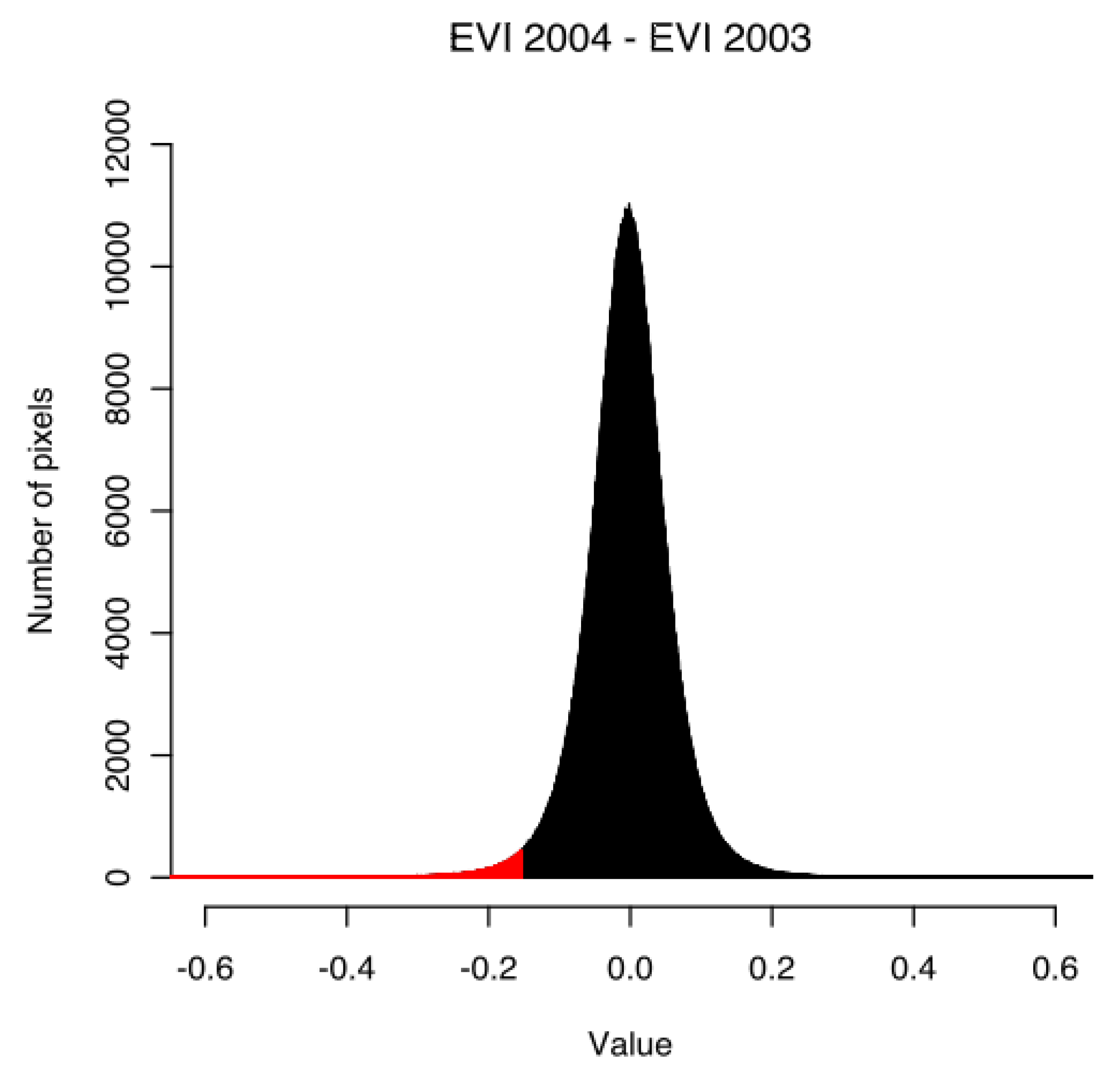
We were able to automatically determine the threshold that yielded the highest concordance between interpreted and modelled deforestation events. After 33 iterations, PEST estimated that the best detection threshold had a value of −0.1570. This meant that if the EVI value of a pixel of a given composite annual EVI image drops by more than 0.1570 compared to the EVI value of that same pixel in the assembled image of the previous year, it would be identified as a hotspot for deforestation.
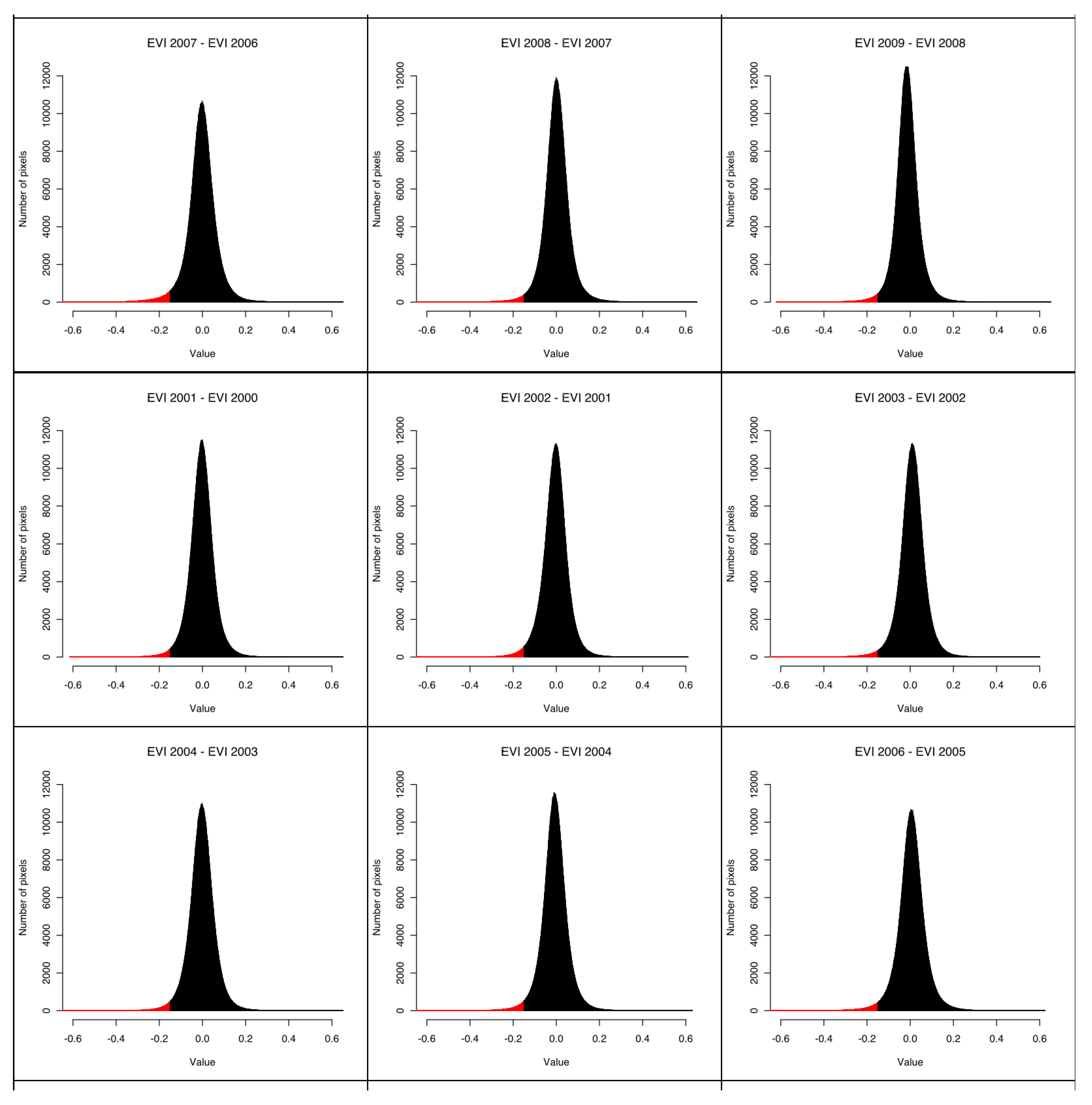
Figure 5 shows the histogram of the image produced by subtracting the 2003 EVI image from the 2004 EVI, with pixels marked in red where hotspots were detected. As
Figure 6 shows, the histograms of all nine differentiated images are similar. This is to be expected as the MODIS team, using a systematic workflow, consistently produces the EVI data we used.
Figure 5.
Histogram of the differentiated EVI images of 2004 and 2003 with pixels representing hotspots highlighted in red according to a −0.1570 detection threshold.
Figure 5.
Histogram of the differentiated EVI images of 2004 and 2003 with pixels representing hotspots highlighted in red according to a −0.1570 detection threshold.
Figure 6.
Histogram of the nine differentiated EVI images with pixels representing hotspots highlighted in red according to a detection threshold of −0.1570.
Figure 6.
Histogram of the nine differentiated EVI images with pixels representing hotspots highlighted in red according to a detection threshold of −0.1570.
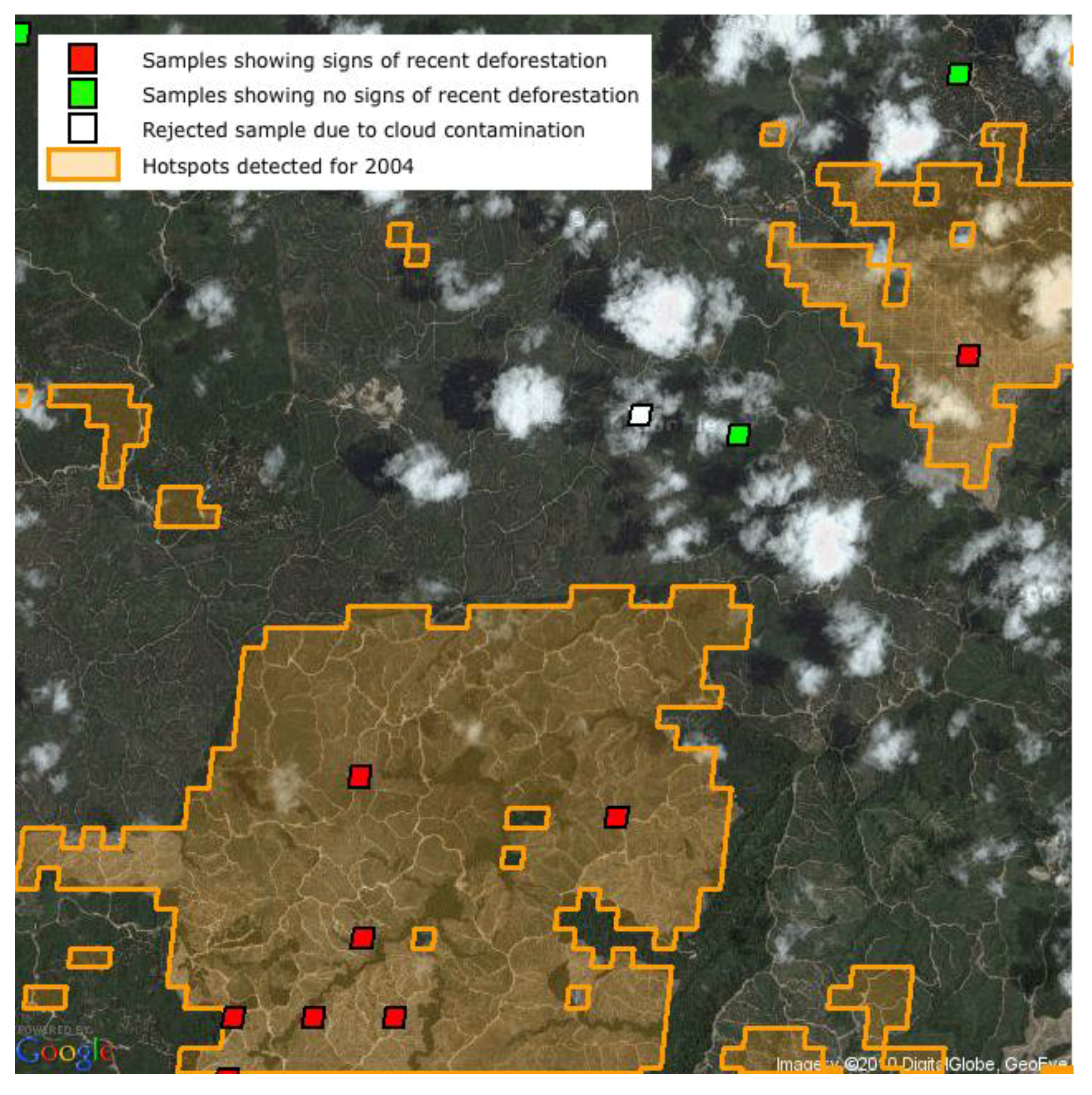
3.3. Estimation of Hotspot Locations
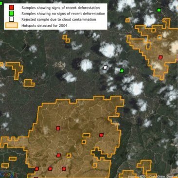
Figure 7 shows a portion of high-resolution imagery and the validation data that was sampled over this area. Each sample is represented by a colored polygon in the shape of a rhombus, equal in size to a MODIS dataset pixel. These polygons are aligned to the MODIS raster grid. Areas showing recent signs of deforestation as well as areas that show none have been sampled. Since the image in
Figure 7 was taken on 27 February 2005, we know that the deforestation events sampled, displayed in red, happened before that date: that is, sometime before and up to the year 2005. For this reason, hotspots should be detected in MODIS imagery for these pixels sometime between 2001 and 2005 inclusively. As the orange overlay shows, hotspots were indeed detected for these samples in 2004. Similarly, no hotspots should be detected over areas sampled that show no sign of deforestation, displayed in green, up to the year 2004 inclusively. One sample, displayed in white, was rejected because of cloud contamination and not considered further in the detection threshold estimation process.
Figure 7.
Samples of a Google Earth high-resolution image taken on 27 February 2005 with an overlay of the hotspots detected for the year 2004 [
8].
Figure 7.
Samples of a Google Earth high-resolution image taken on 27 February 2005 with an overlay of the hotspots detected for the year 2004 [
8].
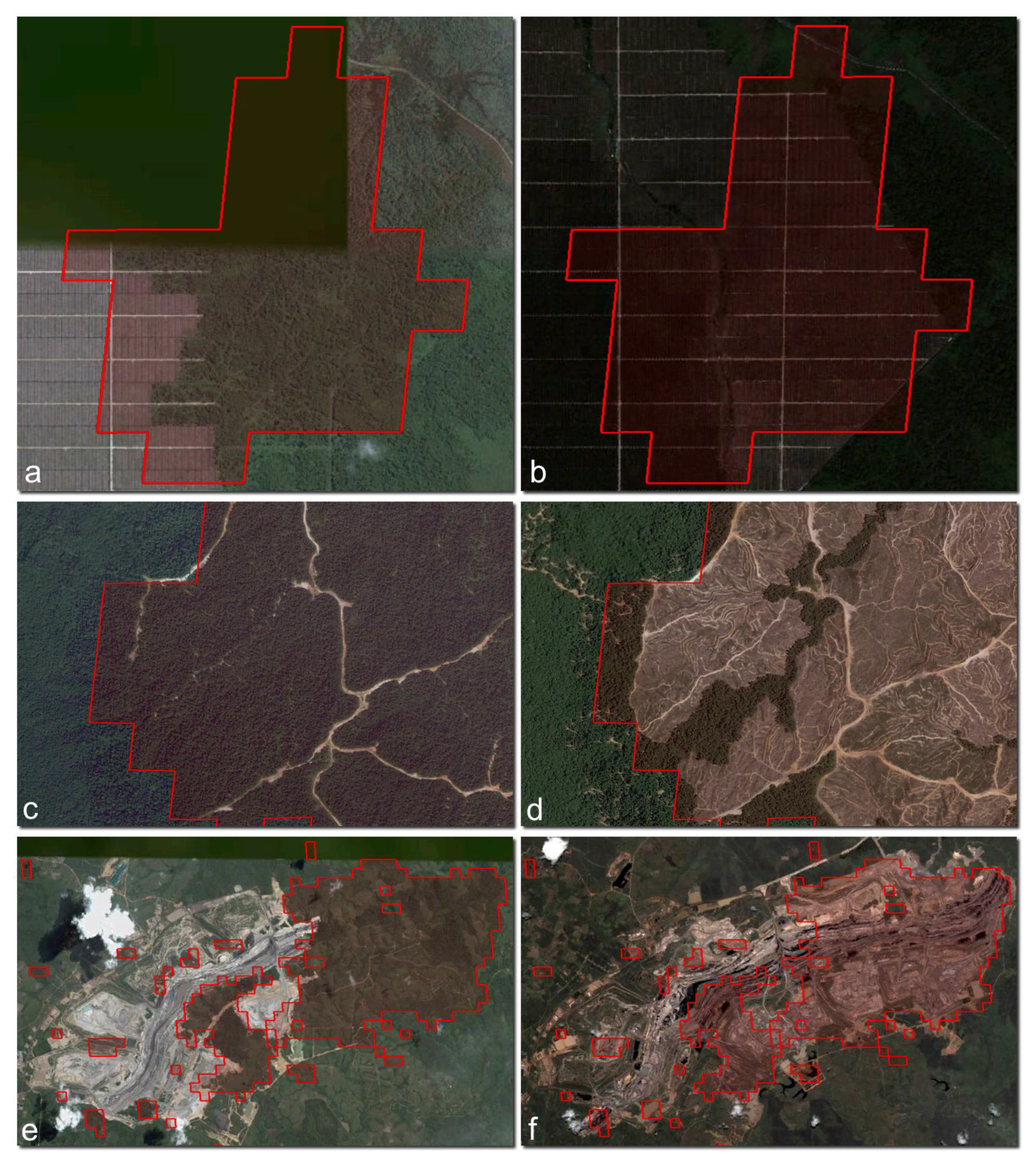
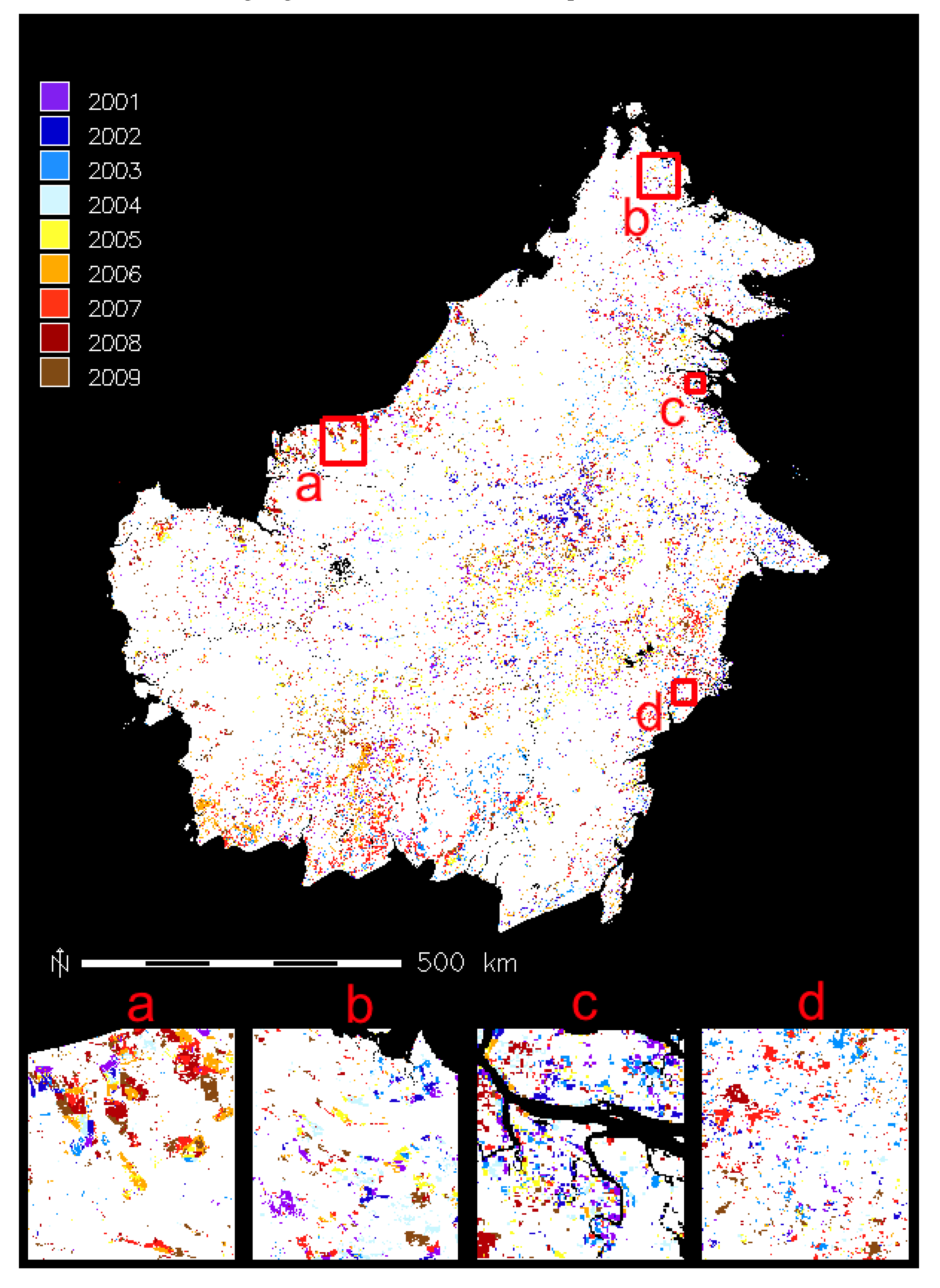
Using our methodology, we have produced nine maps representing yearly deforestation hotspots in Borneo. As
Figure 8 shows, the hotspots we have mapped can correspond to actual deforestation events. By combining the nine maps we have created into a single document (
Figure 9), we can see that spatio-temporal patterns are present. For instance, we can see hotspots on
Figure 9(a) that evolve in a front-like manner from year to year. This type of pattern is typical of the powerful deforestation vectors present in Borneo such as plantation expansion, forestry activities and, to a lesser extent, urban sprawl. Small hotspots, such as those found on
Figure 9(b), are common as well. They testify to the diverse nature of land use conversion that prevails in Borneo. True, industrial forestry and palm oil production put a lot of pressure on Borneo’s forest, but smaller phenomenon also have effects. For instance, the impacts of small landowners and indigenous populations that exploit the land might also be responsible for some hotspots.
Figure 8.
(a) and
(b) Hotspots detected in 2007 from MODIS imagery overlaid on a 2004 Google Earth image
(a) and on an image from 2009 2009
(b) high-resolution Google Earth image.
(c) and
(d) Hotspots detected in 2004 from MODIS imagery overlaid on a 2003
(c) and a 2005
(d) high-resolution Google Earth image.
(e) and
(f) Hotspots detected in 2005, 2006, 2007 and 2008 from MODIS imagery overlaid on a 2004
(e) and a 2009
(f) high‑resolution Google Earth image [
8].
Figure 9.
Yearly deforestation hotspots detected in between the year 2001 and the year 2009 in Borneo, with highlighted areas shown in lower panels.
Figure 9.
Yearly deforestation hotspots detected in between the year 2001 and the year 2009 in Borneo, with highlighted areas shown in lower panels.
4. Discussion
As much as it is tempting to further analyze trends from the hotspots maps we have produced, we must remain cautious. The hotspots that are mapped do not necessarily correspond to actual deforestation events. Conversely, not all deforestation is correctly detected. The first aim of hotspot cartography is to aid the targeted monitoring efforts seeking areas that are likely to have undergone deforestation [
4,
27,
28]. Using methods such as remote sensing based on medium and high-resolution data or in situ verification for wall-to-wall forest monitoring of large territories like Borneo is intensive in terms of computational, human and financial resources. Furthermore, geographical particularities of some areas of the world, namely the abundant cloudiness that affect regions such as Borneo, make high-resolution wall-to-wall monitoring of forests virtually impossible. Focusing
in situ verification and high-resolution remote sensing efforts to areas identified as hotspots make it possible to monitor Borneo’s forests in a way that is both logistically and financially sensible.
The hotspots detected do not encompass all the deforestation events that might have occurred. Likewise, it is not possible to know with certainty if the hotspots correspond to deforestation without resorting to higher resolution data or in situ verification. Beyond this limitation of hotspot cartography, there are other limitations that are inherent in our methodology. For instance, using the EVI to detect changes that affect forest cover can also lead to false positives for certain types of land covers. The types of land covers involved are those where, in contrast to most of the evergreen forests of Borneo, large variations in the value of the EVI happen year round. For instance, the EVI can vary significantly in healthy, undisturbed peat swamps as the level of the water table fluctuates. If it drops for some time, the vegetation can dry out and turn yellow. This translates into a decrease of EVI. When the water table level increases again, the vegetation replenishes and the EVI increases.
Similarly, false positives can also be detected on land used for agriculture where ever-changing EVI values can be observed. This is because the EVI over a cultivated piece of land displays a cyclic behavior. The cycle starts with bare land with a low EVI. The EVI increases as the plants grow and then drops abruptly with the harvest.
The way we produce composite images also introduces limitations. For example, the number of pixels used to determine the value of a pixel in an assembled image is variable. For some areas that are severely plagued by atmospheric contamination, no pixels are usable at all. Thus, the assembled images’ quality is uneven and they remain partially, though mostly, complete.
5. Conclusions
Despite these limitations, hotspot detection can prove quite useful within a broader monitoring protocol. As such, it is bound to play an important role in the support of deforestation mitigation initiatives, such as
Reducing Emissions from Deforestation and Degradation plus (REDD-plus). Although the implementation of REDD-plus is still the subject of heated debate in the international community, there is a consensus that it is necessary to implement it rapidly [
29]. Consequently, REDD-plus projects are already taking shape in some parts of the world, including Borneo [
30,
31]. The monitoring of forests, and namely the carbon-rich rainforests such as those that are found in Borneo, is going to be an important part of REDD-plus. Hotspot detection based on coarse satellite data will likely be a part of the related monitoring efforts. Even though it can be quite a challenge to do remote sensing in very humid parts of the world, the techniques we have used show that it is feasible even on a limited budget.
Because of widely available free software and the growing GIS-like capabilities of Google Earth, only modest resources are needed to produce maps like the ones in our hotspots time series. The availability of freely distributed or viewed data such as MODIS and Google Earth high-resolution images, as well as free software like PEST and GRASS GIS, reduces the overhead cost of the infrastructure necessary for systematic forest monitoring. Together, these valuable resources can help the remote sensing community gather useful results, even if financial resources are limited. Moreover, cost effectiveness is especially important in parts of the world like Borneo, where the regions to survey are vast and funding must be stretched as much as possible.
Borneo’s forests are still actively being cut down by the forestry and palm oil industries. With the emergence of international initiatives such as REDD-plus, there is hope that the remaining natural habitats might get some level of protection. If successful, REDD-plus will not only serve the global population by mitigating climate change, it will also serve the local communities, the first beneficiaries of their natural environments, and it will help slow down the loss of the heavily threatened biodiversity of Borneo.
Acknowledgments
This project was supported by the Canadian Government through the SSHERC/CRSH program on the grant entitled “Expansion agricole, déforestation, biocarburants, marché mondial: Bornéo au cœur de la tourmente.” We thank Rodolphe De Koninck, Stéphane Bernard, Mark Girard, Luke Southwell and Vincent Chai for the valuable help they have provided in the realization of this project.
References
- Cardille, J.A.; Bennett, E.M. Ecology: Tropical teleconnections. Nature Geosci. 2010, 3, 154–155. [Google Scholar] [CrossRef]
- DeFries, R.S.; Rudel, T.; Uriarte, M.; Hansen, M. Deforestation driven by urban population growth and agricultural trade in the twenty-first century. Nature Geosci. 2010, 3, 178–181. [Google Scholar] [CrossRef]
- Malhi, Y. The carbon balance of tropical forest regions, 1990–2005. Current Opinion Environ. Sustain. 2010, 2, 237–244. [Google Scholar] [CrossRef]
- DeFries, R.; Achard, F.; Brown, S.; Herold, M.; Murdiyarso, D.; Schlamadinger, B.; de Souza, C., Jr. Reducing Greenhouse Gas Emissions from Deforestation in Developing Countries: Considerations for Monitoring and Measuring; GOFC-GOLD Report Series 26; Global Terrestrial Observing System: Rome, Italy, 2006. [Google Scholar]
- GPCP. Animation of Version 2 Monthly Precipitation Images (January 1979 to February 2001); Braun, S., Ed.; NASA/GSFC: Pasadena, CA, USA, 2011. [Google Scholar]
- Langner, A.; Miettinen, J.; Siegert, F. Land cover change 2002–2005 in Borneo and the role of fire derived from MODIS imagery. Glob. Change Biol. 2007, 13, 2329–2340. [Google Scholar] [CrossRef]
- Cihlar, J. Land cover mapping of large areas from satellites: Status and research priorities. Int. J. Remote Sens. 2000, 21, 1093–1114. [Google Scholar] [CrossRef]
- Google Inc. Google Earth 6; Google Inc.: Mountain View, CA, USA, 2011; Available online: http://www.google.com/earth/ (accessed on 1 June 2011).
- Vancutsem, C.; Pekel, J.F.; Bogaert, P.; Defourny, P. Mean compositing, an alternative strategy for producing temporal syntheses. Concepts and performance assessment for SPOT VEGETATION time series. Int. J. Remote Sens. 2007, 28, 5123–5141. [Google Scholar] [CrossRef]
- Stibig, H.J.; Beuchle, R.; Achard, F. Mapping of the tropical forest cover of insular Southeast Asia from SPOT4-Vegetation images. Int. J. Remote Sens. 2003, 24, 3651–3662. [Google Scholar] [CrossRef]
- Bontemps, S.; Defourny, P. Mapping Forest Change in Borneo in 2000–2006 by a Multispectral Statistically-Based Detection Technique with SPOT-VEGETATION. In Proceedings of the 2007 International Workshop on the Analysis of Multi-Temporal Remote Sensing Images, Leuven, Belgium, 18–20 July 2007.
- NASA. MODIS Web. Available online: http://modis.gsfc.nasa.gov/about/ (accessed on 1 June 2011).
- Huete, A.; Justice, C.; van Leeuwen, W. MODIS Vegetation Index (MOD13), Algorithm Theoretical Basis Document, April 1999.
- Masuoka, E.; Fleig, A.; Wolfe, R.E.; Patt, F. Key characteristics of MODIS data products. IEEE Trans. Geosci. Remote Sens. 1998, 36, 1313–1323. [Google Scholar] [CrossRef]
- Huete, A.; Didan, K.; Miura, T.; Rodriguez, E.P.; Gao, X.; Ferreira, L.G. Overview of the radiometric and biophysical performance of the MODIS vegetation indices. Remote Sens. Environ. 2002, 83, 195–213. [Google Scholar] [CrossRef]
- Lu, D.; Mausel, P.; Brondizio, E.; Moran, E. Change detection techniques. Int. J. Remote Sens. 2004, 25, 2365–2407. [Google Scholar] [CrossRef]
- Cardille, J.A.; Foley, J.A. Agricultural land-use change in Brazilian Amazonia between 1980 and 1995: Evidence from integrated satellite and census data. Remote Sens. Environ. 2003, 87, 551–562. [Google Scholar] [CrossRef]
- Knorn, J.; Rabe, A.; Radeloff, V.C.; Kuemmerle, T.; Kozak, J.; Hostert, P. Land cover mapping of large areas using chain classification of neighboring Landsat satellite images. Remote Sens. Environ. 2009, 113, 957–964. [Google Scholar] [CrossRef]
- Standart, G.D.; Stulken, K.R.; Zhang, X.; Zong, Z.L. Geospatial visualization of global satellite images with Vis-EROS. Environ. Model. Softw. 2011, 26, 980–982. [Google Scholar] [CrossRef]
- GRASS Development Team. Geographic Resources Analysis Support System (GRASS GIS) Software; Open Source Geospatial Foundation: Vancouver, BC, Canada, 2010. [Google Scholar]
- Taylor, F. Google Earth 5—Historical Imagery. Google Earth Blog 2009.
- Clemo, T.; Christensen, S.; Cosgrove, D.; Dahlstrom, D.; Dausman, A.; Fienen, M.; Gallagher, M.; Hunt, R.; James, S.; Johnson, G.; Keating, E.; Langevin, C.; Moore, C.; Muffels, C.; Shook, M.; Tonkin, M.; Schreuder, W.; Welter, D.; Wylie, A.; Young, S.; Zyvoloski, G. PEST: Model-Independent Parameter Estimation and Uncertainty Analysis; PEST, Echo Valley Graphics, Inc.: Bernville, PA, USA, 2010. [Google Scholar]
- Land Processes Distributed Active Archive Center. Vegetation Indices 16-Day L3 Global 250 m; USGS: Sioux Falls, SD, USA, 2008.
- Land Processes Distributed Active Archive Center. Vegetation Indices 16-Day L3 Global 250 m; USGS: Sioux Falls, SD, USA, 2007.
- Land Processes Distributed Active Archive Center. Vegetation Indices 16-Day L3 Global 250 m; USGS: Sioux Falls, SD, USA, 2009.
- Land Processes Distributed Active Archive Center. Vegetation Indices 16-Day L3 Global 250 m; USGS: Sioux Falls, SD, USA, 2010.
- DeFries, R.; Asner, G.; Achard, F.; Justice, C.; Laporte, N.; Price, K.; Small, C.; Townshend, J. Monitoring tropical deforestation for emerging carbon markets. In Tropical Deforestation and Climate Change; Moutinho, P., Schwartzman, S., Eds.; Amazon Institute for Environmental Research: Belém, Pará, Brazil, 2005; pp. 35–46. [Google Scholar]
- DeFries, R.; Achard, F.; Brown, S.; Herold, M.; Murdiyarso, D.; Schlamadinger, B. Earth observations for estimating greenhouse gas emissions from deforestation in developing countries. Environ. Sci. Policy 2007, 10, 385–394. [Google Scholar] [CrossRef]
- UNFCCC Copenhagen Accord. Available online: http://unfccc.int/files/meetings/cop_15/application/pdf/cop15_cph_auv.pdf (accessed on 1 June 2011).
- Downer, A.; Wirajuda, H. Kalimantan Forest and Climate Partnership; Austrilia Government: Canberra, ACT, Australia, November, 2008.
- International Forest Carbon Initiative. Kalimantan Forest and Climate Partnership Factsheet; Australian Government Initiative; Austrilia Government: Canberra, ACT, Australia, December 2009.
© 2011 by the authors; licensee MDPI, Basel, Switzerland. This article is an open access article distributed under the terms and conditions of the Creative Commons Attribution license (http://creativecommons.org/licenses/by/3.0/).


