Accuracy Enhancement of ASTER Global Digital Elevation Models Using ICESat Data

Abstract

Global Digital Elevation Models (GDEM) are considered very attractive for current research and application areas due to their free and wide range accessibility. The ASTER Global Digital Elevation Model exhibits the highest spatial resolution data of all global DEMs and it is generated for almost the whole globe. Unfortunately, ASTER GDEM data include many artifacts and height errors that decrease the quality and elevation accuracy significantly. This study provides a method for quality improvement of the ASTER GDEM data by correcting systematic height errors using ICESat laser altimetry data and removing artifacts and anomalies based on a segment-based outlier detection and elimination algorithm. Additionally, elevation errors within water bodies are corrected using a water mask produced from a high-resolution shoreline data set. Results indicate that the accuracy of the corrected ASTER GDEM is significantly improved and most artifacts are appropriately eliminated. Nevertheless, artifacts containing lower height values with respect to the neighboring ground pixels are not entirely eliminated due to confusion with some real non-terrain 3D objects. The proposed method is particularly useful for areas where other high quality DEMs such as SRTM are not available.

1. Introduction

Global Digital Elevation Models (GDEM) which are freely available for all users and accessible via the Internet are used for many applications in several disciplines. GDEMs are provided in different resolutions, are generated by employing various techniques, and exhibit different ranges of coverage on the earth’s surface. Recently, in July 2009, the Ministry of Economy, Trade, and Industry (METI) of Japan and the United States National Aeronautics and Space Administration (NASA) released a new GDEM, which is a great step towards a worldwide high-resolution elevation model. It is produced from Advanced Spaceborne Thermal Emission and Reflection Radiometer (ASTER) stereo images. The aim of the ASTER GDEM is to provide a highly accurate DEM, which covers the complete landmass, and is freely available to all users. Furthermore it is aimed to be used as a platform for analysis of data in the fields of disaster monitoring (e.g., volcanic or flood hazard map), hydrology (e.g., water resource management), energy (e.g., oil resource exploration), and stereoscopic visualization (e.g., for Bird’s-eye views and flight simulations) [1]. The ASTER GDEM is generated with a spatial resolution of about 30 m (1 arc-second) from the original 15 m ASTER image ground sampling distance (GSD) in the horizontal plane. Therefore, the ASTER GDEM is the highest resolution DEM among the free accessible global DEMs. Other important GDEMs include the Shuttle Radar Topography Mission (SRTM) DEM with a resolution of 3 arc-seconds (∼90 m at the equator) and the Global Topographic Data (GTOPO30) with a resolution of 30 arc-seconds (∼1,000 m at the equator).

The ASTER GDEM covers land surfaces between −83${}^{\circ }$ and +83${}^{\circ }$. Moreover, the ASTER GDEM data are available also for those high latitude and steep mountainous areas that are not covered by SRTM (available between −58${}^{\circ }$ and +60${}^{\circ }$) due to orbit restrictions, radar shadowing, and foreshortening effects [1].

The vertical and horizontal accuracies of ASTER GDEM are estimated in pre-production level at 95% confidence as 20 m, and 30 m respectively. Prior to releasing the ASTER GDEM data to the global user community in July 2009, an extensive preliminary validation study in cooperation with the US Geological Survey (USGS), ERDAS, and other investigators has been performed [2]. The results of the accuracy assessment by this study prove that the pre-production estimated vertical accuracy of 20 m at 95% confidence is globally correct. Looking to single tiles of size 1${}^{\circ }$× 1${}^{\circ }$, some exhibit a vertical accuracy of better than 20 m but for others the accuracy can be worse. The study concludes that the major errors of the GDEM are the following issues:

• The ASTER GDEM shows almost for all areas a general negative bias of about 5 m on average. The comparison in the Continental United States (CONUS) proves that the ASTER GDEM is on average about 4 m lower than the National Elevation Dataset (NED), and more than 6 m lower in open and flat regions.
• The GDEMs data contain artifacts and anomalies, which can produce large elevation errors on local scales. These errors occur mainly in areas where just few stereo images are available or in the regions with persistent “clouds”. Artifacts due to existing small numbers of stereo images appear as straight lines, “pits”, “bumps”, “mole-runs”, and other geometric shapes [2].
• In the ASTER GDEM, no inland water mask has been applied and therefore the elevation values on most of the lakes are inaccurate, i.e., the elevation values of water body regions are not set to a single “flattened” height value.

Therefore, the major motivation of the work in this paper is to provide methodologies to generate an improved and thus more appropriate digital elevation model, in particular for the areas where the SRTM data are not available, i.e., above 60${}^{\circ }$ North and below 58${}^{\circ }$ South. Accordingly, in this paper the quality of the ASTER GDEM is improved. This is performed by using the ICESat laser altimetry data for absolute height improvement and some local refinement measures. Huber et al. [3] proposed an algorithm for correcting the height accuracy of the SRTM DEMs using the ICESat laser altimetry points. The Geoscience Laser Altimeter System (GLAS) instrument mounted on ICESat (Ice, Cloud, and land Elevation Satellite), measures elevation data since 2003. The absolute height accuracy of the laser points varies depending on land cover and relief and it is generally better than 1 m [4]. GLAS produces a series of approximately 70 m diameter footprints that are separated by nearly 170 m intervals along track and 30 km across track (at the equator) and 5 km at 80${}^{\circ }$ latitude [5]. Huber et al. [3] proposed a strategy to refine and extract high quality laser points from the ICESat waveform dataset to be applied for SRTM DEM correction. They investigate the deviation of ICEsat points from a reference Digital Surface Model (DSM) (with accuracy of ±0.5 m in open areas and ±1.5 m in areas covered with vegetation) and a reference Digital Terrain Model (DTM) (with accuracy of ±0.5 m). As final refinement, the selected parameters of the laser waveform, i.e., received energy, signal width, peak numbers, and standard deviation, has been adapted to attain highly accurate laser points. The final height accuracy of the selected ICESat points after employing the predefined criteria are obtained as 0.64 m mean and 1.30 m standard deviation regarding the investigated 65 points. As further work, they have proposed an algorithm to enhance the global elevation quality of SRTM data using the selected ICESat points. It is assumed that the SRTM data contains long wavelength errors up to a level of 10 m [6]. Therefore, a model for long wavelength errors based on spherical harmonics has been generated in which the coefficients of the model are estimated by a least squares adjustment based on the differences between ISESat and SRTM. The method based on spherical harmonics correction function calculates continuously the error offset to SRTM rather than adding only one offset value for each tile.

While spherical harmonic functions are suitable in case of solving long wavelength errors, this is not the case for the ASTER GDEM. The ASTER GDEM is based on a group of individual acquisitions and not on continuously acquired stripes as it is the case for SRTM DEM.

The overall goal of this paper is to enhance the quality of the ASTER GDEM with focus on the regions where SRTM DEM is not available. Hence, the paper has the following objectives:

• Correction of the height offset errors by employing selected ICESat laser altimetry data as control points. A correction layer is generated by measuring the deviation of the ASTER GDEM from the corresponding ICESat laser point.
• Removal of local artifacts and anomalies using a segmentation-based method.
• Modifying the height of pixels of the lakes and water bodies by employing a water mask layer provided by an existing freely accessible water boundary database.

2. Methods

According to the errors reported in the first ASTER GDEM validation report [2], summarized in Section 1, a methodology is proposed in this paper to reduce and correct the three errors in the following three steps:

2.1. Correction of the Height Errors Using ICESat Laser Altimetry Points:

The focus is on the refinement of the elevation data by reducing the ASTER GDEM bias based on a correction layer, which is provided from the ICESat laser altimetry data. For that, a correction height layer is provided according to the height deviation of the ASTER GDEM points from the corresponding ICESat points.

As first step, the ICESat point clouds corresponding to the test area are extracted from the dataset repository. In order to use the ICESat points as Ground Control Points (GCPs) to be applied on evaluation and correction of the DEMs, the erroneous points caused by clouds, outliers, underlying slopes or vegetation should be eliminated first. Based on the criteria proposed by Huber et al. [3], the points containing errors are filtered to reach a vertical accuracy of nearly 1 m compared to the reference data. Accordingly, the ICESat waveform laser points are filtered by selecting appropriate thresholds for different parameters as follows: (1) number of peaks as a criterion to distinguish bare soil and forest areas, (2) received energy from signal begin to signal end, and (3) the signal width (in meter), which is the distance between signal begin and signal end.

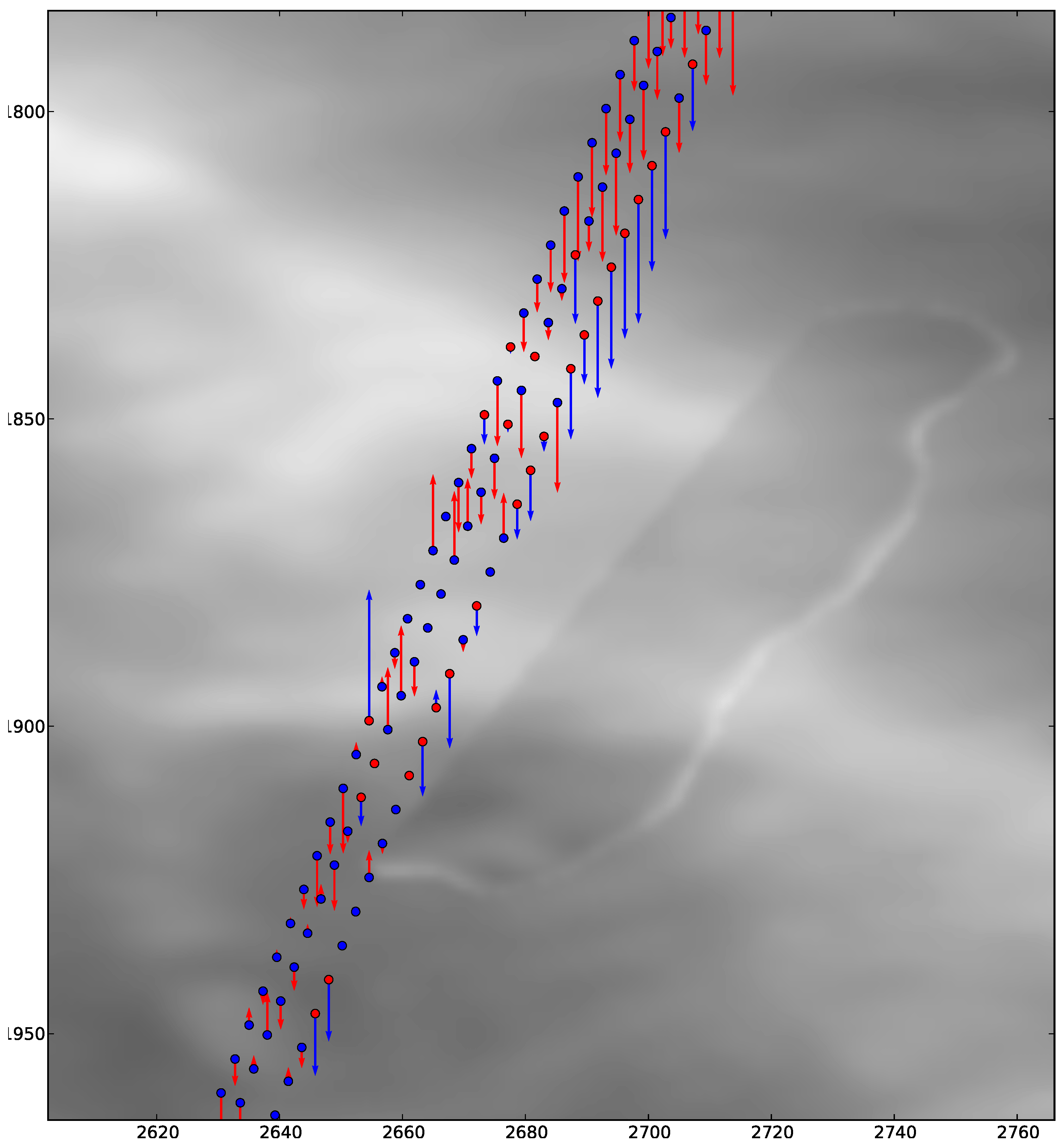
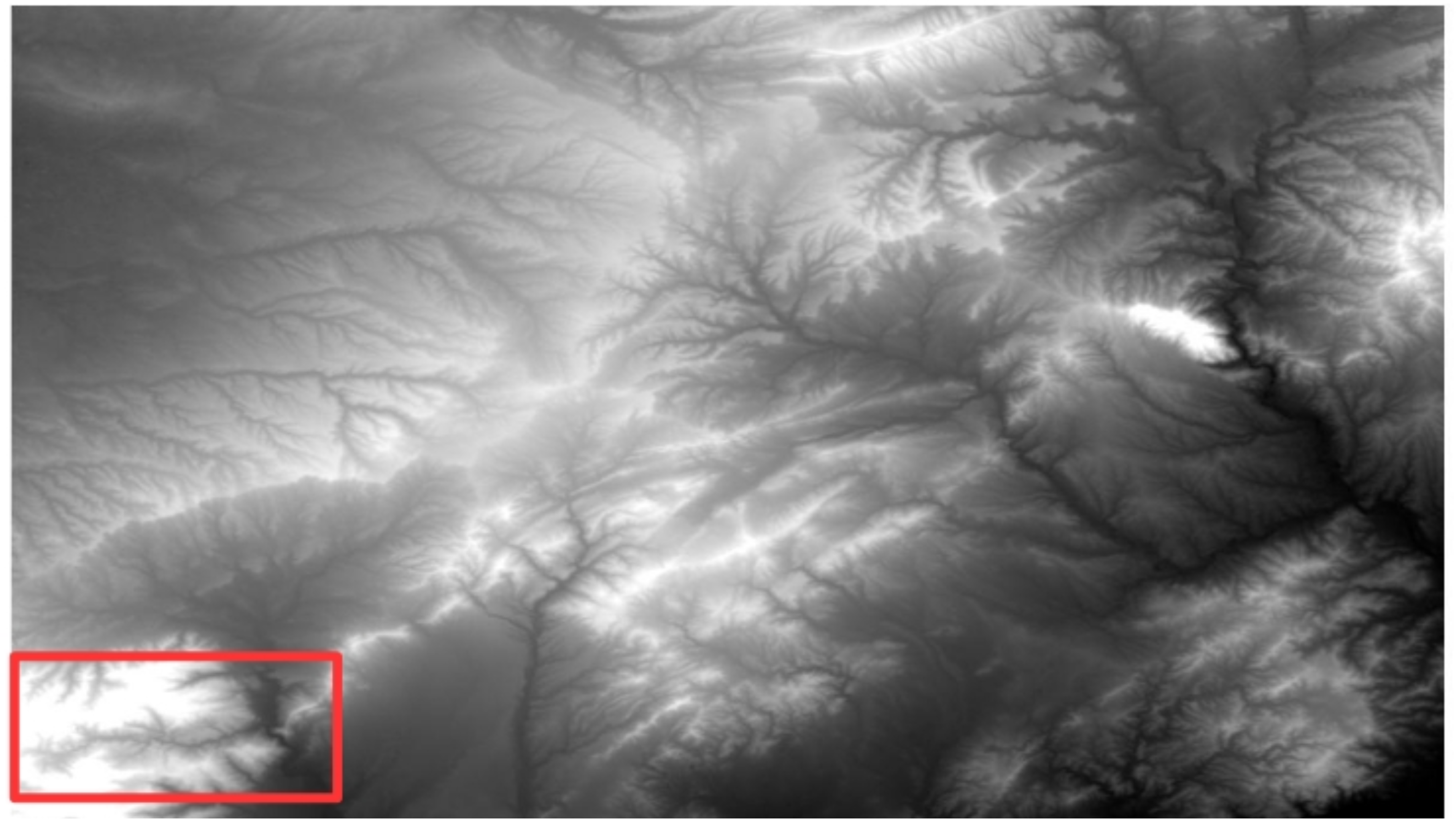
Figure 1 represents the locations of the ICESat laser altimetry data over a sample of ASTER GDEM data. It additionally shows the direction and magnitude of the height deviation of the GDEM regarding the ICESat points. The direction of the vertical arrows proves that the ASTER GDEM is located generally below the correct elevation. The original laser points located in the region are refined using the parameters recommended by Huber et al. [3] as follows: Points with less than 6 peaks, received energy lower than 10 fJ (femtojoule), and a signal width smaller than 25 m are selected. The ICESat points that are not satisfying all the predefined criteria are eliminated from the dataset. They are visualized as blue arrows in Figure 1.

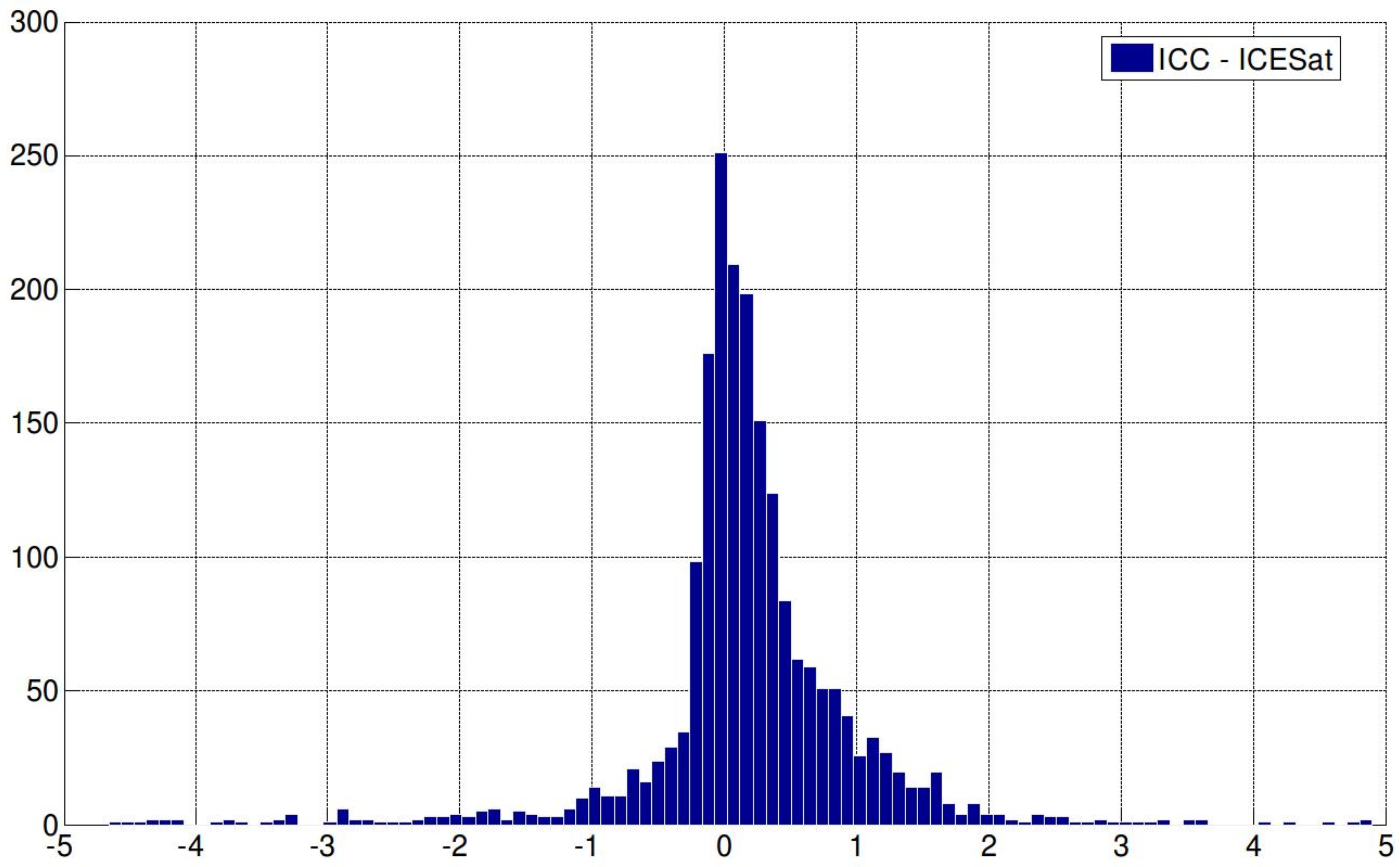
After selecting the corresponding ICESat points and their correction, in order to obtain high accuracy points, analogous ASTER GDEM points are extracted using interpolation. An additional criterion is utilized to reject the ICESat laser points that are not consistent with the GDEM points considering them as outliers. In this step, the aim is to obtain the vertical offsets related to each ASTER GDEM point to reduce the negative bias of the ASTER GDEM. For that purpose the difference between the selected ICESat points and their corresponding ASTER GDEM points are measured. A correction height layer is provided by interpolation of the height differences within the test area (cf. Figure 2).

In practice, in order to increase the quality of the correction layer and to be able to apply the algorithm more globally, an area much larger than the test area is analyzed for extracting ICESat points as well as the corresponding GDEM points. This procedure has two benefits: (1) since the ICESat points are not as dense as the GDEM points, selecting a larger area allows to more precisely measure the height offset for the corresponding area, and (2) extracting the ICESat points for a larger area and applying the correction layer only on the test region provides a smooth transition on overlapping areas between neighboring scenes. For the interpolation of the height differences over the entire scene, an ordinary Moving Average method is employed. It assigns the values to the grid nodes by averaging the data within a search ellipse around each node.

Figure 1. ICESat points located on the ASTER GDEM, corresponding to an area of 6 km × 5.1 km plus vector arrows showing the vertical errors of each point. Refined ICESat points to get points located only on the ground surface (red arrows) as well as eliminated points (blue arrows) are visualized.

Figure 1. ICESat points located on the ASTER GDEM, corresponding to an area of 6 km × 5.1 km plus vector arrows showing the vertical errors of each point. Refined ICESat points to get points located only on the ground surface (red arrows) as well as eliminated points (blue arrows) are visualized.

2.2. Segment-Based Artifacts and Anomalies Detection and Elimination:

In this step, an algorithm is proposed to detect and remove artifacts and anomalies as outliers from the ASTER GDEM based on a segmentation. The algorithm to extract and eliminate the artifacts and anomalies from the ASTER GDEM using segmentation technique has been reported in an earlier work of the authors [7].

Figure 2. Elevation correction layer corresponding to an area of about 30 km × 30 km. The values on the X and Y axis represent the pixel coordinates.

Figure 2. Elevation correction layer corresponding to an area of about 30 km × 30 km. The values on the X and Y axis represent the pixel coordinates.

In order to extract the outliers effectively, their types and specifications are identified first. The specifications of the common errors existing in the released ASTER GDEM, which are detailed in ASTER GDEM validation report [2], are summarized as follows:

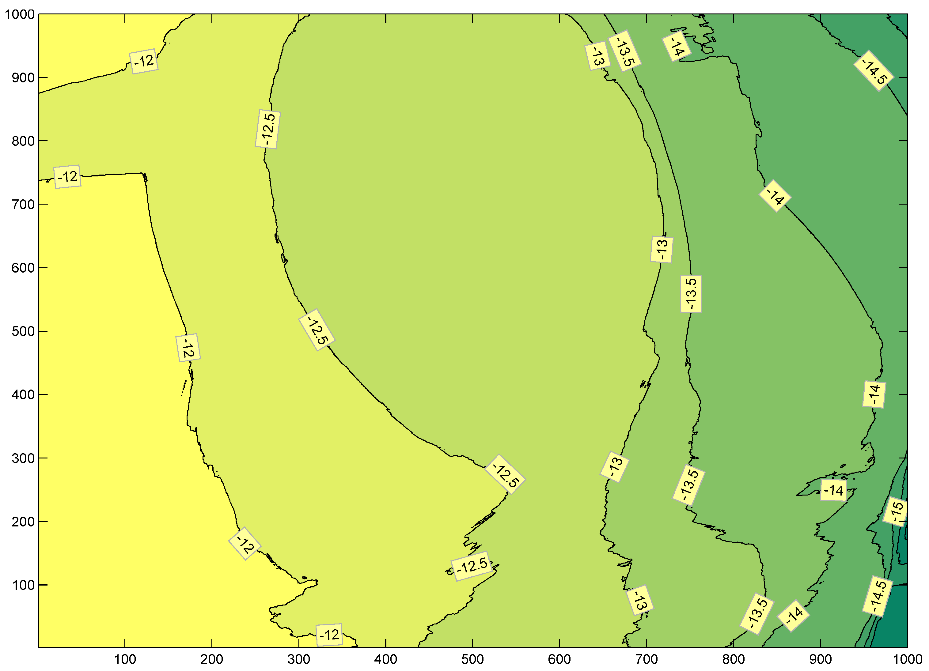
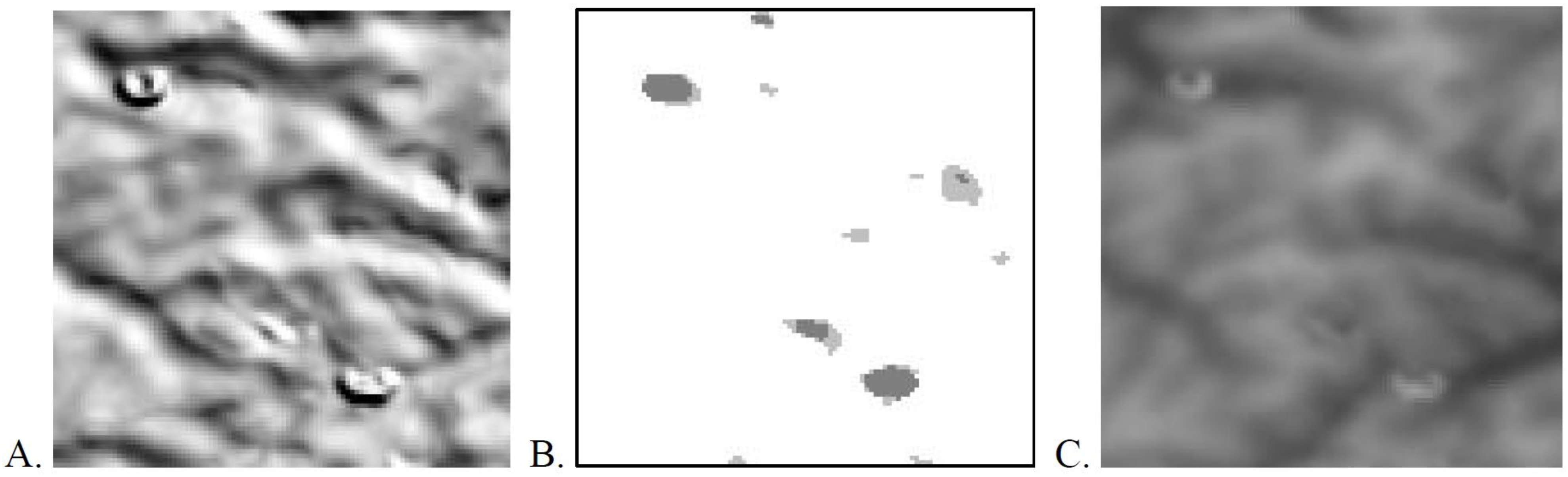
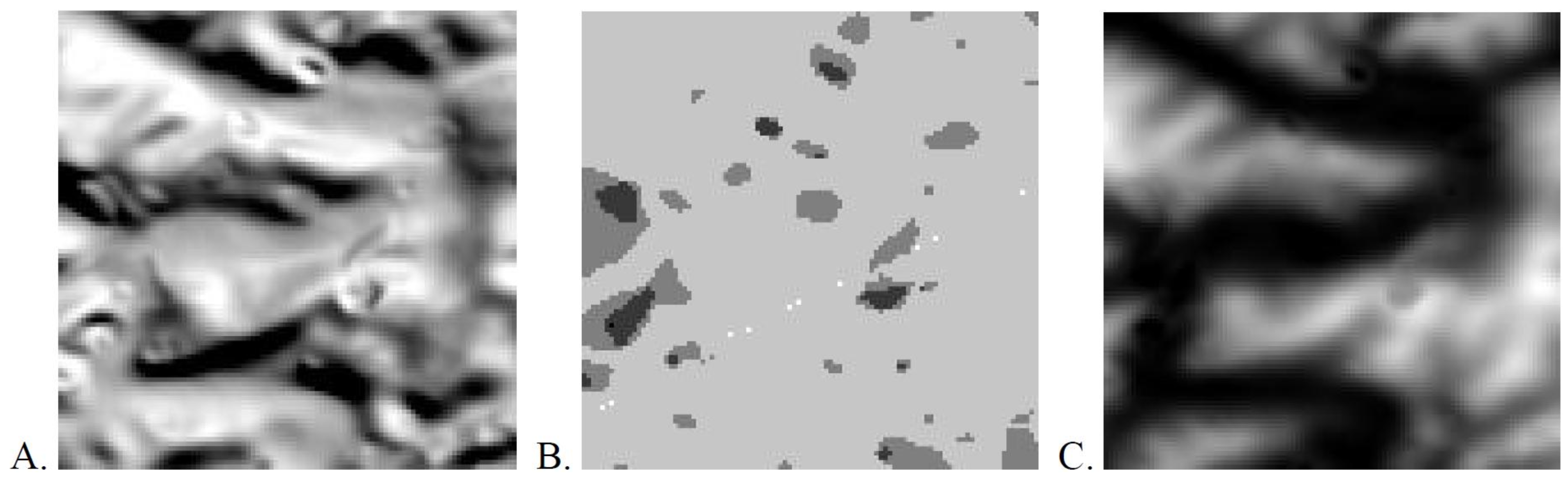
• “Pits” occur as small negative elevation anomalies, which vary from a few meters to about 100 m in height. Figure 3 illustrates an example of the area containing the “pit” artifacts and their association with stack number boundaries (cf. Figure 3(B)). Stack numbers correspond to the number of image pairs that are using to generate DEM.

Figure 3. Example of “pit” artifacts; (A) shaded relief, (B) clear relation to the stack (scene) number boundaries, (C) appearance in ASTER GDEM represented as gray scale image (originally appeared in [8]).

Figure 3. Example of “pit” artifacts; (A) shaded relief, (B) clear relation to the stack (scene) number boundaries, (C) appearance in ASTER GDEM represented as gray scale image (originally appeared in [8]).

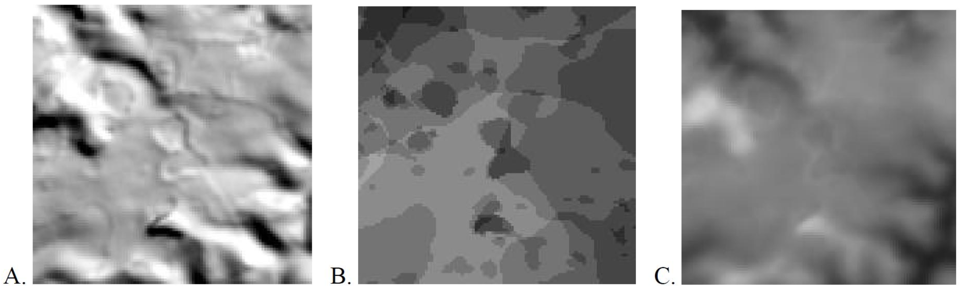
• “Bumps” appear as positive elevation anomaly artifact; their magnitude can range from just few meters to more than 100 m in height (cf. Figure 4).

Figure 4. Example of “bump” artifacts; (A) shaded relief, (B) clear relation to the stack number boundaries, (C) appearance in ASTER GDEM image (originally appeared in [8]).

Figure 4. Example of “bump” artifacts; (A) shaded relief, (B) clear relation to the stack number boundaries, (C) appearance in ASTER GDEM image (originally appeared in [8]).

• “Mole runs” are curvilinear anomalies above the ground, which are less common than pits and bumps and occur in relatively flat terrains. The corresponding magnitude of “mole runs” is much less than for the two previous anomalies and it ranges from barely perceptible to a few meters, and rarely more than 10 m (cf. Figure 5). Due to their linear behavior, they can be easily recognized in a shaded DEM.

Figure 5. Example of “mole-run” artifacts; (A) shaded relief, (B) clear relation to the stack number boundaries, (C) less obvious in ASTER GDEM image (originally appeared in [8]).

Figure 5. Example of “mole-run” artifacts; (A) shaded relief, (B) clear relation to the stack number boundaries, (C) less obvious in ASTER GDEM image (originally appeared in [8]).

The artifacts and anomalies produced by small and different stack numbers are apparent in almost all ASTER GDEM tiles. In addition, the effects of residual clouds have been already eliminated in Version 1 of the ASTER GDEM by replacing the elevation with −9999 values [2]. Here, an algorithm based on image reconstruction using geodesic morphological dilation [9,10] is employed to extract the regional extrema, which is later used for eliminating the “pits” and “bumps”. Geodesic dilation from gray-scale mathematical morphology differs to basic dilation where an image and a structuring element are involved in the filtering process. In geodesic dilation the dilated image is additionally “masked” with a predefined “mask” image. Equation (1) shows the geodesic dilation of image J (marker) using mask I. In most applications, the marker image is defined by a height offset to the mask image, which generally represents the original DEM. 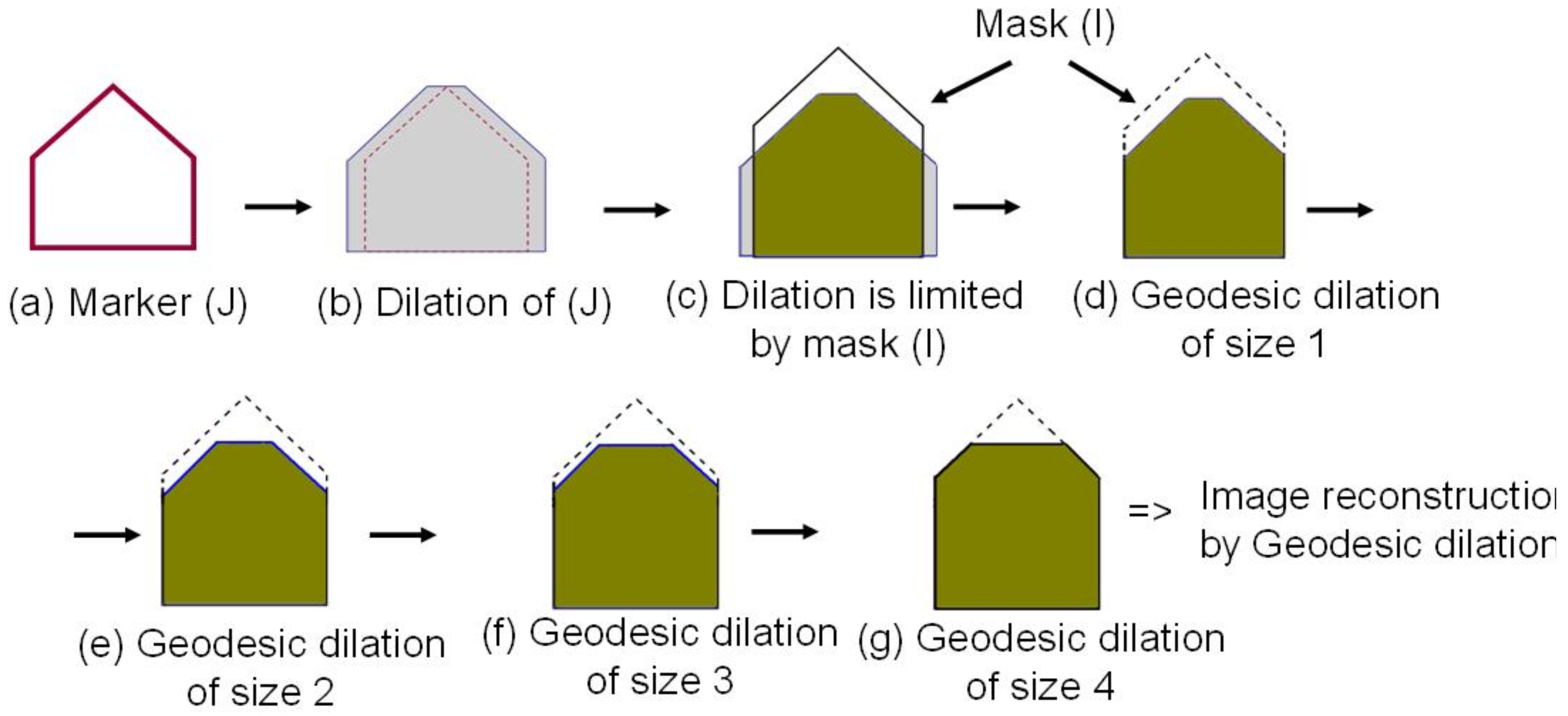Figure 6 illustrates the difference between geodesic and basic image dilation as well as reconstruction based on geodesic dilation in a profile view of a simple building with gable roof. The input image (a), here called marker, is enlarged by dilation, i.e., the gray region in (b), and limited by the mask image (I). The result of geodesic dilation is shown in (d) with a dashed line around it depicting the mask image. If this process, i.e., dilation and limitation by mask, is iteratively continued, it stops after four iterations reaching stability. The result provided by this step is called reconstruction of marker (J) by mask (I) using geodesic dilation (cf. Figure 6(g)). The number of iterations, i.e., n in Equation (2), to create reconstructed image varies from one sample to another. In the example presented in Figure 6 the reconstruction procedure stops after four iterations.

Figure 6. Geodesic dilation.

Figure 6. Geodesic dilation.

Accordingly, geodesic dilation (${\delta }_I$ ) and image reconstruction are defined as

$${\delta }_I^{\left(1\right)}\left(J\right)=(J⨁B)\bigwedge I,$$

(1)

$$\underset{ntimes}{\underbrace{{\delta }_I^{\left(n\right)}\left(J\right)={\delta }_I^{\left(1\right)}\left(J\right)\circ {\delta }_I^{\left(1\right)}\left(J\right)\circ ....\circ {\delta }_I^{\left(1\right)}\left(J\right)}}$$

(2)

Equation (2) defines the morphological reconstruction of the marker image (J) based on geodesic dilation (${\delta }_I$) (cf. Equation (1)) if the iterative geodesic dilations reaches to stability. The basic dilation (δ) of marker and point-wise minimum (∧) between dilated image and mask (I) is employed iteratively until stability. Looking at the reconstructed image of the example depicted in Figure 6 shows that the upper part of the object, i.e., the difference between marker and mask is suppressed during image reconstruction. Therefore, the result of gray scale reconstruction depends on the height offset between the marker and the mask images and accordingly, different height offset suppress different parts of the object. More information regarding the segmentation of the DEMs by gray scale reconstruction using geodesic dilation can be found in [11] where similar algorithms are employed for extracting 3D objects as well as the ridge lines from high resolution LIDAR DSM. In a segmentation algorithm based on geodesic reconstruction, selecting an appropriate “marker” image plays the main role and has a direct effect on the quality of the final reconstructed image. A “marker” image with a small offset, e.g., few meters, from the “mask” can suppress mainly local maxima regions similar to artifacts above the ground.

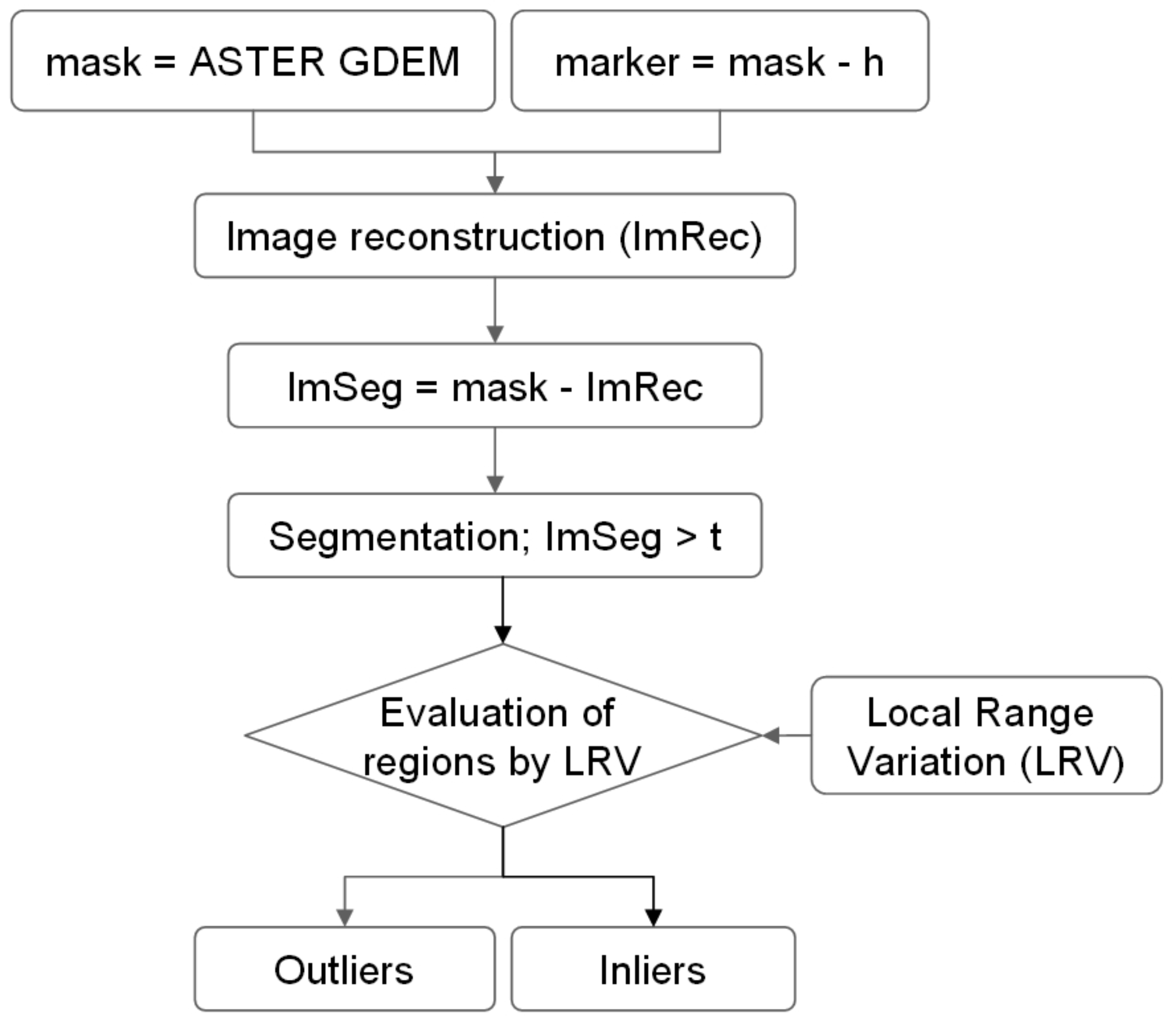
The proposed outlier extraction algorithm regarding the positive artifacts and anomalies is represented in Figure 7. The first step for segmentation based outlier detection is to generate the “marker” image as a second input image. The first input image is the original ASTER GDEM as “mask” image. The marker is generated by subtraction of an offset value h from the ASTER GDEM:

$$mas{k}^{+}=GDEM$$

$$marker=mas{k}^{+}-h$$

where $mas{k}^{+}$ is the “mask” image employed to extract the “positive” outliers. Since the artifacts are in most cases located far beyond the ground elevation level with low height variation of their internal pixels, a single offset value (h) of about “25 m” generates an appropriate marker image for segmentation of the outliers for ASTER GDEM. This is a basic assumption for the outlier elimination algorithm. It means if an outlier region contains low inclination on most parts of its boundary to the neighboring ground pixels, the algorithm might fail to detect it.

Figure 7. Proposed workflow for extracting positive outliers.

Figure 7. Proposed workflow for extracting positive outliers.

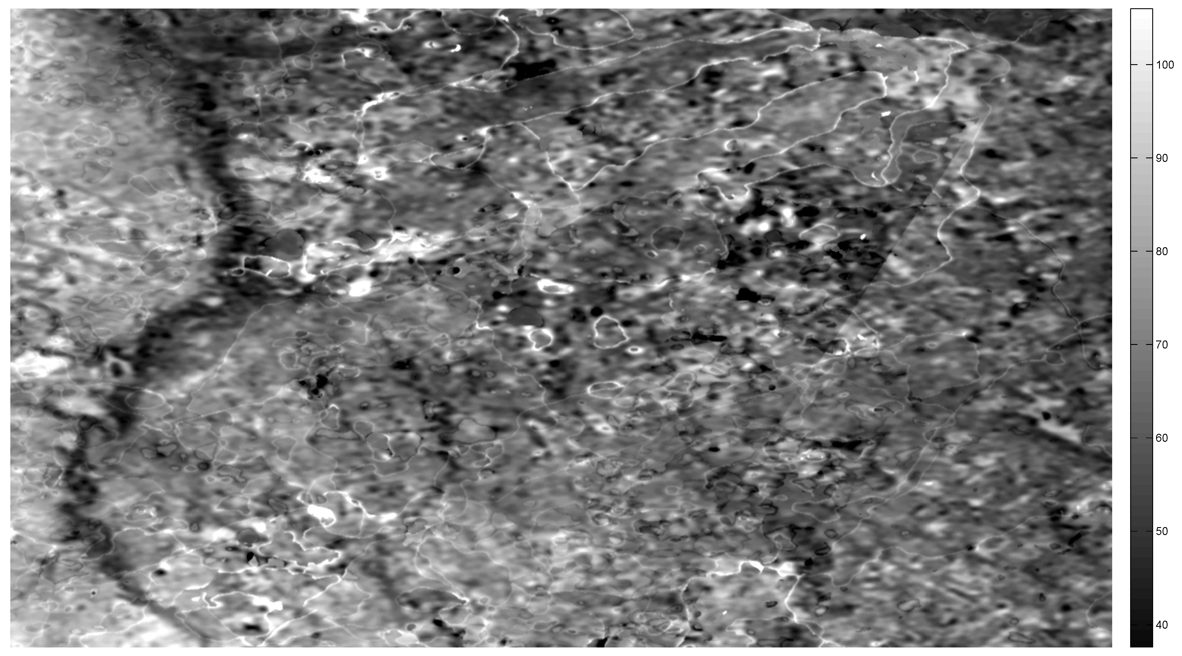
Figure 8 shows a small ASTER GDEM tile with 420 × 550 pixels which is used as “mask” in this algorithm. After providing the second input image (“marker”), the image reconstruction ImRec is determined accordingly. For segmentation purpose, the reconstructed image is subtracted from the original DEM. The result is a normalized DEM similar to normalized Digital Surface Model (nDSM) where the regions which are about h meter higher than their neighborhood are highlighted. Similar results can be achieved by morphological “tophat” filtering [12,13], but the operation based on geodesic dilation is better suited because of its independence from the size of the objects to be filtered. Therefore, there is no need to tune the size of the structuring element.

Figure 8. ASTER GDEM sample data corresponding to an area of 24 km × 39 km.

Figure 8. ASTER GDEM sample data corresponding to an area of 24 km × 39 km.

The segmentation procedure is implemented using thresholding and the labeled regions are provided by means of connected components analysis. A geometric feature descriptor is created which highlights the height variation on each pixel regarding its adjacency to evaluate the labeled regions. A feature called Local Range Variation (LRV) is created by subtracting the maximum and minimum values in every 3×3 windows over the image (cf. Figure 9). All the boundary pixels of the detected regions are evaluated by the LRV descriptor. The regions having certain height jumps on their boundary pixels will be evaluated as outliers (positive artifacts). In practice, the LRV values of the boundary of each region are extracted and if the majority (here 90%) of LRV values are above the threshold (here above 25 m), the region is classified as outlier and corresponding pixels are eliminated from the original data set.

The pixel values corresponding to the LRV are additionally utilized to determine the values that are taken by h (offset from DSM) for automatic generation of the marker image in each iteration. Accordingly the process begins by choosing the maximum value of LRV as initial offset h for marker generation. For an efficient extraction of all outliers, ten offsets are determined by dividing the difference between maximum and minimum LRV into ten equal intervals. The iteration begins with maximum value and the provided segments based on proposed algorithm are evaluated accordingly. Procedure continues by selecting the next h and evaluating the new segments which are not evaluated in previous step until no more new segments are produced. A similar process is utilized to eliminate the negative outliers but in this case, the complementary image of the ASTER GDEM is selected as “mask” and therefore:

$$mas{k}^{-}=max\left(GDEM\right)-GDEM$$

$$marker=mas{k}^{-}-h$$

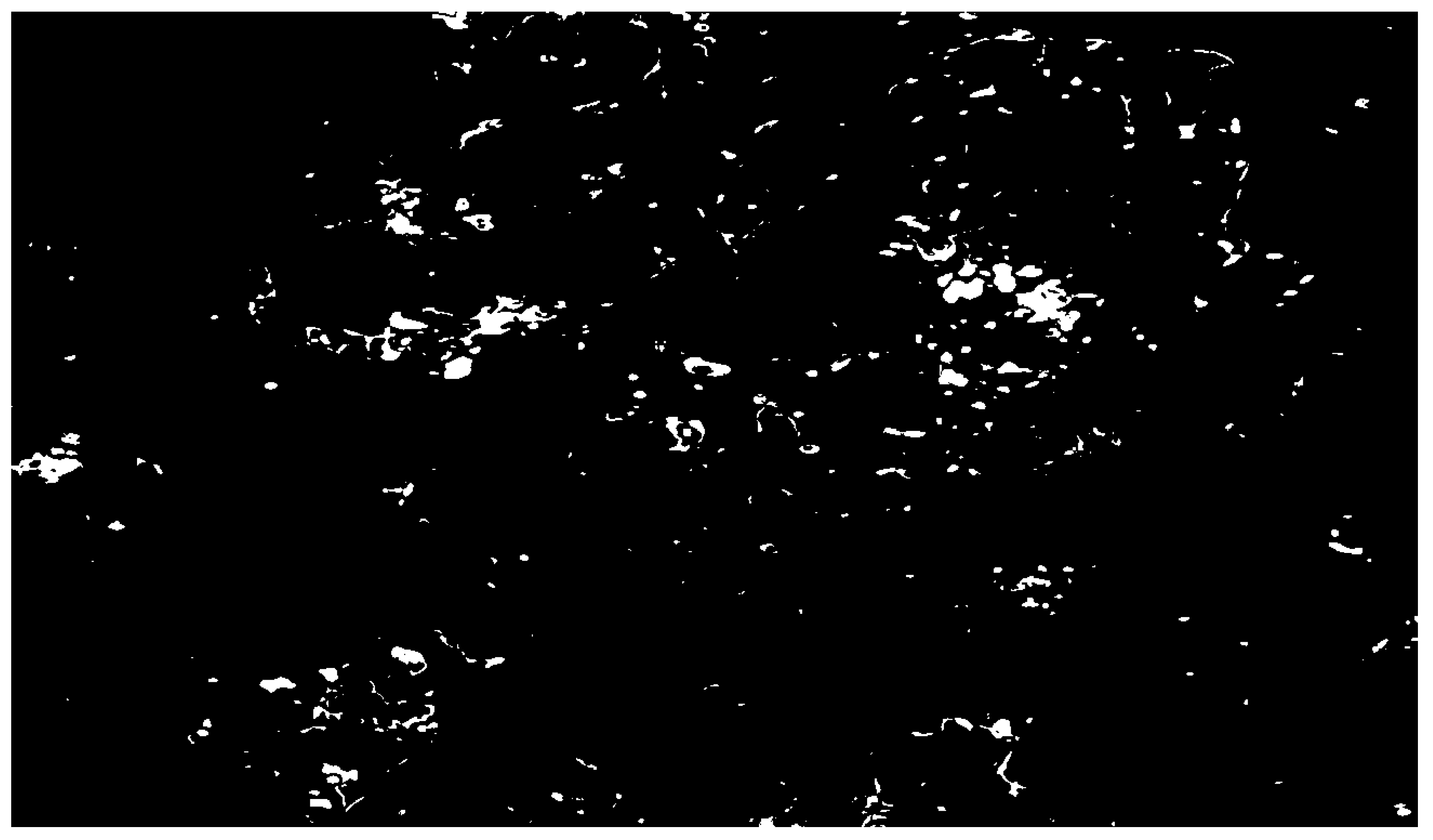
where $mas{k}^{-}$ is used to extract the negative outliers and is created by inverting the original GDEM. Classified outlier regions in this step are then integrated and corresponding pixels are eliminated from the original ASTER GDEM. Figure 10 illustrates the final detected outliers from the example ASTER GDEM image.

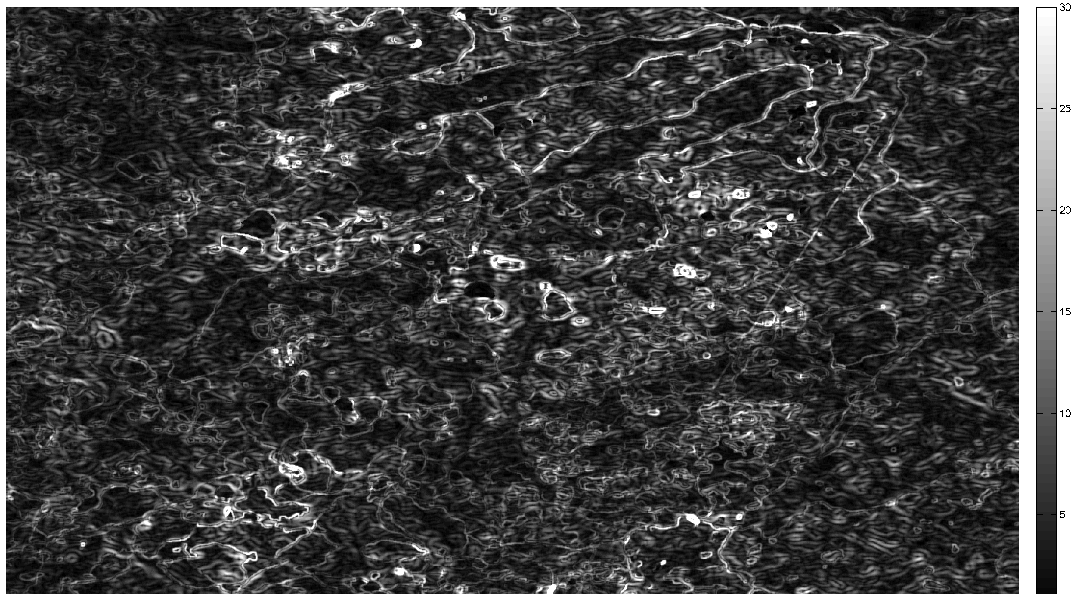
Figure 9. Local Range Variation (LRV) feature descriptor.

Figure 9. Local Range Variation (LRV) feature descriptor.

Figure 10. Final detected positive and negative outliers.

Figure 10. Final detected positive and negative outliers.

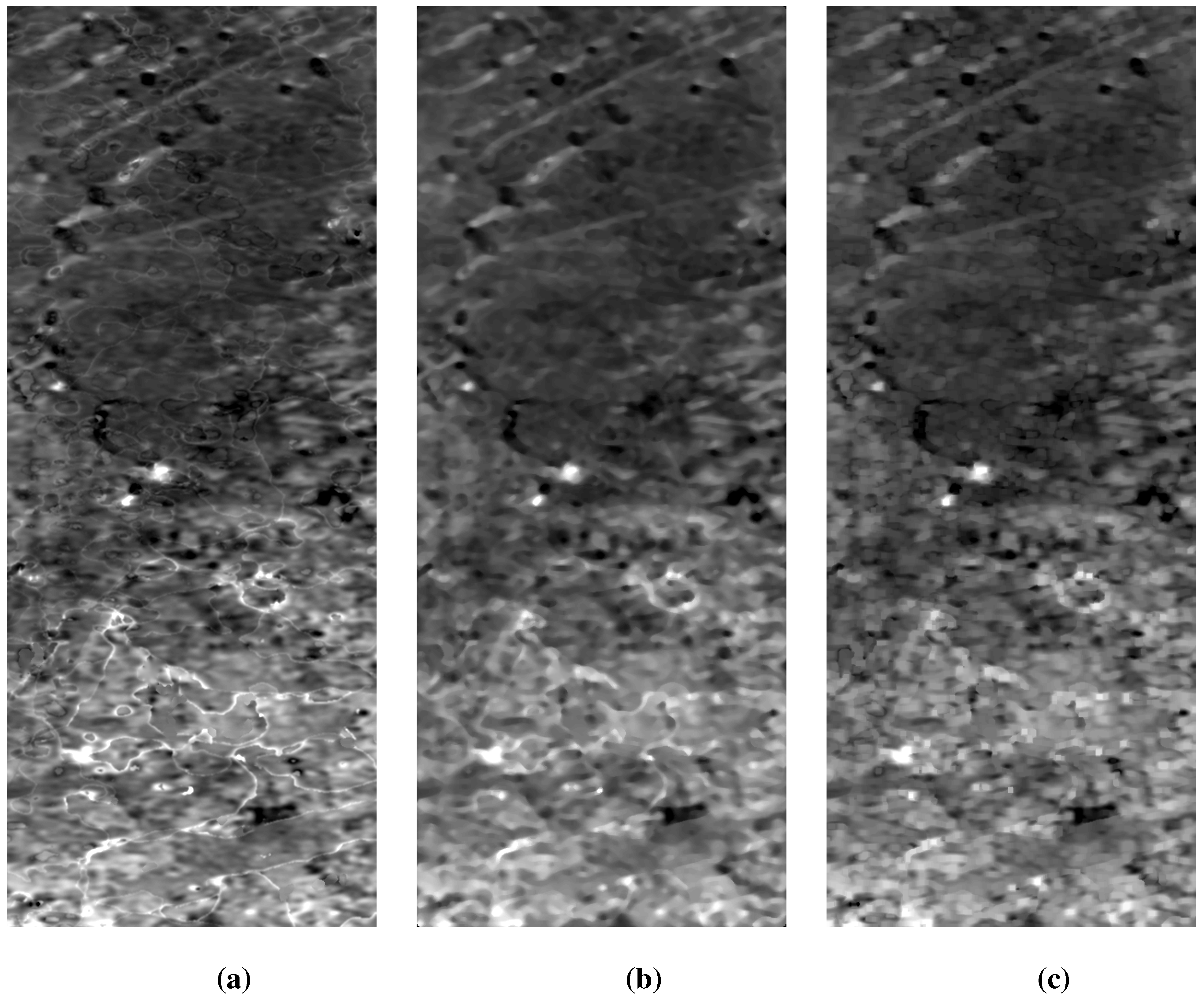
The segment-based algorithm is employed to eliminate the area-shaped artifacts such as “pits” and “bumps”. An additional filtering is integrated to reduce the “mole-runs” errors. Since the “mole-runs” appear as curvilinear and positive height errors, a morphological opening filter is utilized to eliminate them. A disk shaped structuring element with the radius of 7 pixels is selected to suppress curvilinear elevated errors (cf. Figure 11). Median filter is a well-known filtering method of this category, which replaces the value of a pixel by the median of gray values in the neighborhood (cf. Figure 11).

Figure 11. Removal of the curvilinear height errors of “mole-run”. (a) ASTER GDEM; (b) Median filter using a neighborhood image size of 7 × 7; (c) Morphology Opening using a disc shape of radius length of 3 pixels.

Figure 11. Removal of the curvilinear height errors of “mole-run”. (a) ASTER GDEM; (b) Median filter using a neighborhood image size of 7 × 7; (c) Morphology Opening using a disc shape of radius length of 3 pixels.

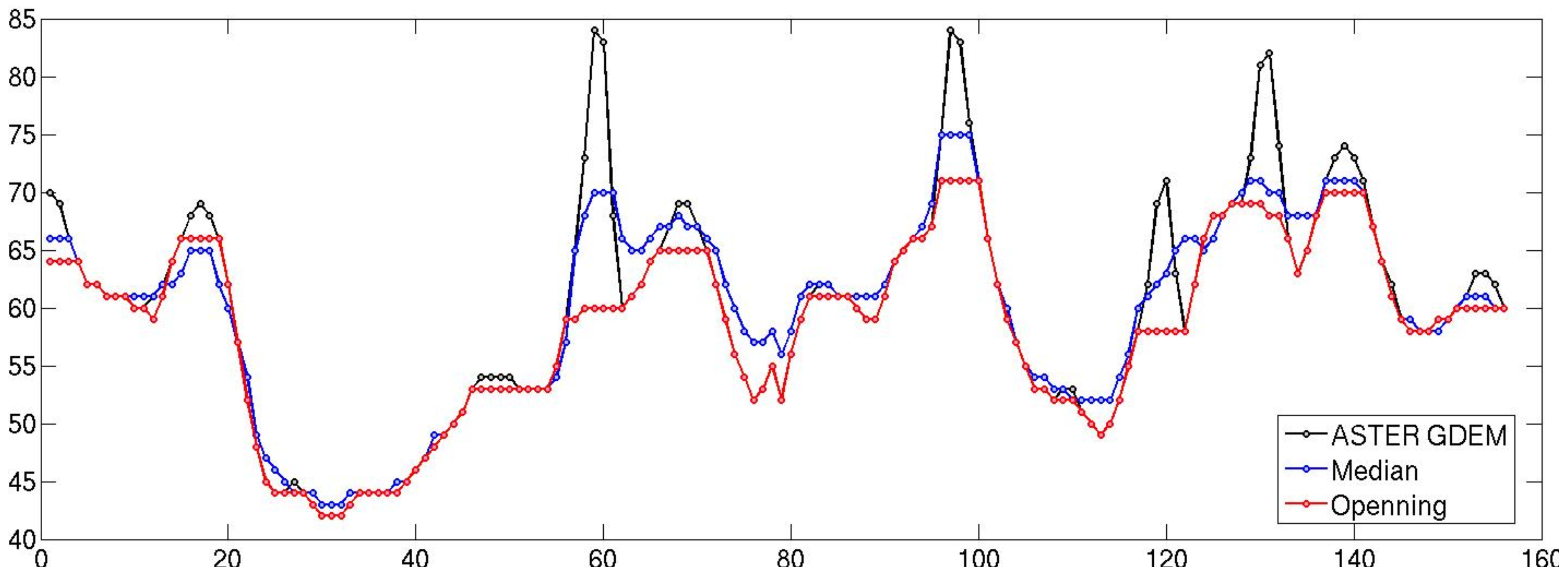
Figure 11 represents the corresponding results by applying median filter and morphological opening on original ASTER GDEM. For the median filter, a neighborhood image size of 7 × 7 is selected for this example which depends on the width of the linear errors to be suppressed. A similar size of structuring element is used for morphological opening to be comparable with the result of median filter. In this work, a disc shaped structuring element with the radius of 3 is employed. To assess the quality of the employed filters for eliminating the mole-runs, a profile plot is provided (cf. Figure 12). In this figure, the black line corresponds to the original ASTER GDEM points where the locations of the several mole-runs as positive peaks are visualized. Median filter (blue line) suppresses parts of the peaks as well as smoothing the other terrain parts. Since the aim is to suppress the sharp peaks with low interference with the other pixels, image opening using an appropriate structuring size creates a better result (cf. Figure 12, red line).

Figure 12. Profiles from images represented in Figure 11, showing that the median filter does not suppress properly the mole-runs errors

Figure 12. Profiles from images represented in Figure 11, showing that the median filter does not suppress properly the mole-runs errors

2.3. Correction of the Height Errors of Water Body Regions:

A further criterion is considered for the final classification into outlier and inliers regions. During production of the ASTER GDEM, the pixels inside inland water bodies are not filtered and, therefore, they contain random errors. In this step, a water mask binary image is provided as a sort of quality layer that warns the user about the lower quality of height points inside water body areas. In addition, the water mask layer can directly be used to filter out all the height points inside the water. In order to provide high quality water mask, the vector map containing the boundary points of the shoreline regions in different resolutions are automatically extracted from the ”Global Self-consistent, Hierarchical, High-resolution Shoreline Database“ (GSHHS) which is is freely available to download [14]. GSHHS is combined from two main databases World Data Bank II (WDB) and World Vector Shoreline (WVS). The shorelines are provided as closed polygons and are free of intersections or other artifacts caused by data inaccuracies [15].

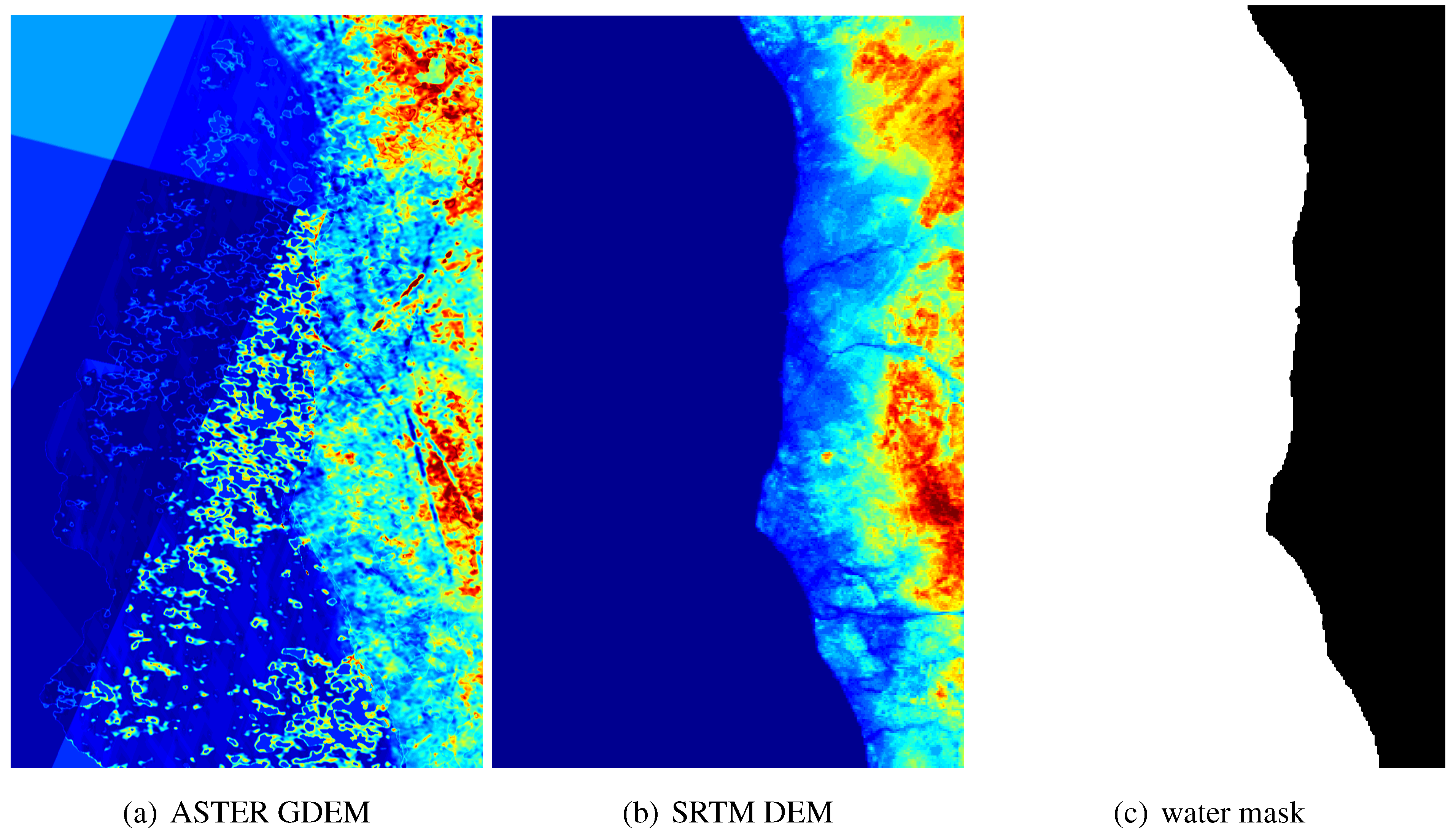
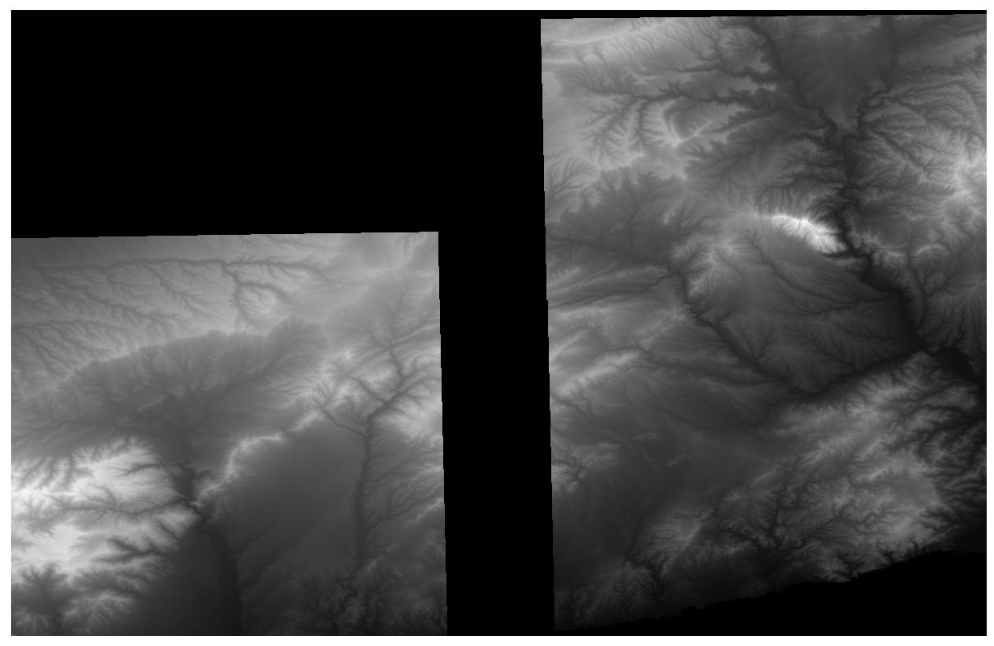
Figure 13(a) shows a small tile of ASTER GDEM corresponding to an area containing a water region with low elevation quality. Comparing to the SRTM image cf. Figure 13(b)), the different blue tones in the water region illustrated that the water region is a merged result of smaller DEMs created from different numbers of stereo scenes (stack numbers). Particularly, such effects occur when the merged DEMs have been generated using a small numbers of stereo scenes. In such situation the quality of SRTM DEM (cf. Figure 13(b)) for the region with small stack numbers are much higher than the ASTER GDEM (cf. Figure 13(a)).

Accordingly, the height values inside the water regions in ASTER GDEM are flattened using the water mask created from the GSHHS data set (cf. Figure 13(c)). After extracting the corresponding water regions, the median value of the associated heights of the boundary region is inserted for the pixels in the related water region. It should be mentioned that, the median of the heights is not applied for rivers. Hence, the difference between the maximum and minimum heights of the boundary pixels are measured. If the difference is less than a predefined value, e.g., 2 m, the median of the heights of the boundary pixels is used as replacement, otherwise the pixels in the region remain intact.

Figure 13. ASTER GDEM, SRTM, and water mask provided by GSHHS data (3 km × 1.4 km).

Figure 13. ASTER GDEM, SRTM, and water mask provided by GSHHS data (3 km × 1.4 km).

An additional check is required to guarantee that the new water level is not higher than the surrounding ground pixels. In case of a higher water level, the median of the lowest 10% of the boundary pixels is considered as water elevation. In the final step, the gaps provided by all the different outliers are filled by applying a spatial interpolation procedure. In this paper, Inverse Distance Weighting (IDW) interpolation [16] is utilized.

3. Results

3.1. Test Data

The proposed algorithms for enhancement of the ASTER GDEM were experimentally tested on a dataset belonging to an area near Barcelona, Spain. The area is selected due to the availability of an accurate ground truth for final evaluation of the corrected DEM. The area is a mountainous region containing 2,378 × 3,601 pixels with a height range from zero up to 1202 m. The data at the southeast part of the scene represent the Mediterranean Sea, which is visible by a very dark gray value (cf. Figure 14).

Figure 14. Original ASTER GDEM; image size = 2378 × 3601 pixels corresponding to 71.3 km × 108 km; Height variation = [0 m, 1202 m].

Figure 14. Original ASTER GDEM; image size = 2378 × 3601 pixels corresponding to 71.3 km × 108 km; Height variation = [0 m, 1202 m].

3.2. ASTER GDEM Enhancement

In the first enhancement step as explained in Section 2.1, a correction layer is provided which represents the vertical offset for each pixel of the GDEM. For this purpose, the ICESat laser altimetry points corresponding to the test area are extracted. A refinement strategy on ICESat waveform laser data is accomplished to reduce the outliers and the laser points located on the top of trees. An additional refinement is considered to eliminate the points with a too high discrepancy to the ASTER GDEM for which a maximum deviation of about 50 m is used. Next, the correction layer is provided by spatial interpolation of the differences between the remaining laser points and the corresponding GDEM points. The correction layer is then employed to shift the original ASTER GDEM pixels according to the values of the correction layer. The second enhancement step is dedicated to the segment-based outlier detection procedure. In this step the common artifacts, which are mentioned in Section 2.2 are detected and eliminated. The curvilinear elevation error, i.e., “mole-run” is reduced by employing a morphological opening filter and the two other errors, “pits” and “bumps”, are eliminated using the segment-based algorithm (cf. Figure 15). As a final process, the gaps created due to outliers are filled by means of spatial interpolation using Inverse Distance Weighting (IDW) [16].

As the third enhancement step, the inland water bodies are extracted from the GSHHS vector database, as explained in Section 2.3. A water mask layer is created by converting the water polygons into a raster image. The process continues by filling corresponding water pixels of GDEM by the median values of the bordering pixels if the region is not regarded as a river.

Figure 15. Outlier regions corresponding to the area indicated in Figure 14 with red polygon; ASTER GDEM (top) and corresponding outliers (bottom).

Figure 15. Outlier regions corresponding to the area indicated in Figure 14 with red polygon; ASTER GDEM (top) and corresponding outliers (bottom).

3.3. Comparison to the Reference DEM

The primary reference dataset used in this evaluation is a bare earth Digital Terrain Model (DTM) produced by the Institut Cartographic de Catalunya (ICC). It has a grid spacing of 15 m and an absolute vertical error of 1.1 m (RMSE). In order to compare it with ASTER GDEM, it has been resampled into 30 m pixel size using bilinear interpolation (cf. Figure 16).

As shown, the ICC ground truth image does not fully cover the whole test area and therefore only the common pixels are assessed in this section. As a first step, the quality of corresponding ICESat and ICC ground truth points are evaluated against each other to check how they fit to each other. A histogram as well as statistical measures are provided to highlight the differences of these two reference datasets (cf. Figure 17 and Table 1). They prove that the ICC ground truth is of very high quality. The average variation of about 18 cm as well as the other parameters, particularly, quantile for 90% of the values demonstrate an appropriate quality as well as a very low rate of outliers.

After evaluating the ground truth the quality of all corrected GDEM points is analyzed against the ICC ground truth. The evaluation includes histograms and determines statistical parameters of the deviations between input and reference datasets. In addition, a profile-view along a specific direction of the ASTER GDEM before and after correction together with the ICC ground truth data shows the improvement visually (cf. Figure 18). In the profiles in Figure 18, the blue lines corresponds to the ICC ground truth data, the red lines show the location of the original ASTER GDEM pixels, and the black lines represent the position of the corrected GDEM pixels.

Figure 16. ICC Ground truth DEM.

Figure 16. ICC Ground truth DEM.

Figure 17. Difference between the ICESat points and ground truth ICC data.

Figure 17. Difference between the ICESat points and ground truth ICC data.

Obviously, the location of the GDEM points after correction is shifted towards the ICC points with much better correspondence. Also local improvements of the DEM shape can be seen in the profile of the corrected data.

Table 1. Comparison of the ground truth against ICESat points.

	Diff. = ICC – ICESat
Min	–4.66 m
Max	4.89 m
Mean	0.18 m
Median	0.13 m
Standard Deviation	0.85 m
RMSE	0.87 m
Quantile 90%	1.01 m

Table 1. Comparison of the ground truth against ICESat points.

	Diff. = ICC – ICESat
Min	–4.66 m
Max	4.89 m
Mean	0.18 m
Median	0.13 m
Standard Deviation	0.85 m
RMSE	0.87 m
Quantile 90%	1.01 m

Figure 18. Profiles compare the location of the ASTER GDEM pixels before (red) and after (black) correction as well as the ICC ground truth (blue).

Figure 18. Profiles compare the location of the ASTER GDEM pixels before (red) and after (black) correction as well as the ICC ground truth (blue).

Figure 19 displays the histograms of the differences between the corrected ASTER GDEM from the ICC points as blue bars overlaid on the histogram of the differences between the original ASTER GDEM and the ICC pixels as red bars. The histograms are corresponding to all the pixels in the common area of the images. The comparison of the two histograms confirms the overall movement of the bias towards a very low value close to zero.

Table 2 represents the statistical measures evaluating the quality of the corrected ASTER GDEM in comparison to the original GDEM. It is obvious that the mean and median measures show almost the same improvement as for the comparison against the ICESat points. The table also shows that the maximum and minimum differences have significantly improved, which is due to eliminating the worst outliers from the scene. Although the standard deviation is reduced by only 0.23 m, this still means that several regions with outliers must have been reduced, which can be partly seen in Figure 18.

Figure 19. Histograms displaying the differences between original ASTER GDEM and ICC ground truth (red) as well as the differences between corrected ASTER GDEM and ICC ground truth.

Figure 19. Histograms displaying the differences between original ASTER GDEM and ICC ground truth (red) as well as the differences between corrected ASTER GDEM and ICC ground truth.

Table 2. Statistical parameters representing the quality improvement of the corrected ASTER GDEM. The ASTER GDEMs before and after correction is compared against the ICC ground truth.

	OrigGDEM – ICC	CorrGDEM – ICC
Min	–193.85 m	–57.36 m
Max	140.05 m	83.66 m
Mean	–12.99 m	0.02 m
Median	–12.78 m	0.03 m
Standard Deviation	8.21 m	7.98 m
RMSE	15.36 m	7.98 m
Quantile 90%	–3.87 m	9.16 m

Table 2. Statistical parameters representing the quality improvement of the corrected ASTER GDEM. The ASTER GDEMs before and after correction is compared against the ICC ground truth.

	OrigGDEM – ICC	CorrGDEM – ICC
Min	–193.85 m	–57.36 m
Max	140.05 m	83.66 m
Mean	–12.99 m	0.02 m
Median	–12.78 m	0.03 m
Standard Deviation	8.21 m	7.98 m
RMSE	15.36 m	7.98 m
Quantile 90%	–3.87 m	9.16 m

4. Conclusions

In this paper, an algorithm consisting of three main steps is proposed for enhancing the quality of the ASTER GDEM. In the first step, the ICESat laser altimetry data are used to provide a correction layer to reduce the height offset of the global DEM.

The second improvement step consists of the reduction of artifacts and outliers from the GDEM, which is performed based on a segment-based algorithm and a smoothing filter. The last step is to flatten the inland water levels by generating a water mask based on the GSHHS shoreline vector dataset. The evaluation based on ground truth data shows that the overall accuracy of the final corrected GDEM is significantly improved and most of the errors and artifacts are removed. Additionally, the water elevation levels are corrected. Moreover, it can be concluded that the ICESat laser points are an appropriate reference data for height correction. In further investigations it is envisaged to correct larger parts of the ASTER GDEM, especially above 60${}^{\circ }$ North and below 58${}^{\circ }$ South and combine SRTM and ASTER GDEM for remaining areas.

References

1. ERSDACT. Earth Remote Sensing Data Analysis Center. Available online: http://www.ersdac.or.jp (accessed on 7 June 2011).
2. ERSDACT(a). ASTER Global DEM Validation Summary Report. Technical Report. Available online: http://www.gdem.aster.ersdac.or.jp (accessed on 7 June 2011).
3. Huber, M.; Wessel, B.; Kosmann, D.; Felbier, A.; Schwieger, V.; Habermeyer, M.; Wendleder, A.; Roth, A. Ensuring Globally the TanDEM-X Height Accuracy: Analysis of the Reference Data Sets ICESat, SRTM and KGPS-Tracks. In Proceedings of IEEE International Geoscience and Remote Sensing Symposium (IGARSS ’09), Cape Town, South Africa, 12–17 June 2009; pp. 769–772.
4. Duong, H.; Lindenbergh, R.; Pfeifer, N.; Vosselman, G. ICESat full-waveform altimetry compared to airborne laser scanning altimetry over The Netherlands. IEEE Trans. Geosci. Remote Sens. 2009, 47, 3365–3378. [Google Scholar] [CrossRef]
5. NASA/ICESat. Available online: http://icesat.gsfc.nasa.gov/ (accessed on 7 June 2011).
6. Rodriguez, E.; Morris, C.; Belz, J.; Chapin, E.; Martin, J.; Daffer, W.; Hensley, S. An Assessment of the SRTM Topographic Products; Technical Report JPL D-31639; Jet Propulsion Laboratory: Pasadena, CA, USA, 2005; p. 143. [Google Scholar]
7. Arefi, H.; Reinartz, P. Elimination of the Outliers from Aster GDEM data. In Proceedings of The 2010 Canadian Geomatics Conference and Symposium of Commission I, ISPRS, Calgary, AB, Canada, 15–18 June 2010; In IAPRS. 2010; Vol. 38. Part 1. [Google Scholar]
8. Abrams, M.; Bryan, B.; Hiroji, T.; Masami, H. The ASTER Global DEM. Photogramm. Eng. Remote Sensing 2010, 76, 344–348. [Google Scholar]
9. Vincent, L. Morphological grayscale reconstruction in image analysis: Applications and efficient algorithms. IEEE Trans. Image Process. 1993, 2, 176–201. [Google Scholar] [CrossRef] [PubMed]
10. Arefi, H.; Hahn, M. A Morphological Reconstruction Algorithm for Separating Off-Terrain Points from Terrain Points in Laser Scanning Data. In Proceedings of the ISPRS Workshop Laser Scanning 2005, Enschede, The Netherlands, 12–14 September 2005; In IAPRS. 2005; Vol. 36. Part 3/W19. [Google Scholar]
11. Arefi, A. From LIDAR Point Clouds to 3D Building Models. Ph.D. Thesis, Bundeswehr University, Munich, Germany, 2009. [Google Scholar]
12. Gonzalez, R.C.; Woods, R.E. Digital Image Processing; Prentice Hall: Upper Saddle River, NJ, USA, 2008. [Google Scholar]
13. Soille, P. Morphological Image Analysis: Principles and Applications, 2nd ed.; Springer-Verlag: Secaucus, NJ, USA, 2003. [Google Scholar]
14. GSHHS—A Global Self-consistent, Hierarchical, Highresolution Shoreline Database. Available online: http://www.ngdc.noaa.gov/mgg/shorelines/gshhs.html (accessed on 7 June 2011).
15. Wessel, P.; Smith, W.H.F. A global self-consistent, hierarchical, high-resolution shoreline database. J. Geophys. Res. 1996, 101, 8741–8743. [Google Scholar] [CrossRef]
16. Haining, R. Spatial Data Analysis: Theory and Practice, 1st ed.; Cambridge University Press: Cambridge, UK, 2003. [Google Scholar]