Evaluating the Remote Sensing and Inventory-Based Estimation of Biomass in the Western Carpathians

Abstract

Understanding the potential of forest ecosystems as global carbon sinks requires a thorough knowledge of forest carbon dynamics, including both sequestration and fluxes among multiple pools. The accurate quantification of biomass is important to better understand forest productivity and carbon cycling dynamics. Stand-based inventories (SBIs) are widely used for quantifying forest characteristics and for estimating biomass, but information may quickly become outdated in dynamic forest environments. Satellite remote sensing may provide a supplement or substitute. We tested the accuracy of aboveground biomass estimates modeled from a combination of Landsat Thematic Mapper (TM) imagery and topographic data, as well as SBI-derived variables in a Picea abies forest in the Western Carpathian Mountains. We employed Random Forests for non-parametric, regression tree-based modeling. Results indicated a difference in the importance of SBI-based and remote sensing-based predictors when estimating aboveground biomass. The most accurate models for biomass prediction ranged from a correlation coefficient of 0.52 for the TM- and topography-based model, to 0.98 for the inventory-based model. While Landsat-based biomass estimates were measurably less accurate than those derived from SBI, adding tree height or stand-volume as a field-based predictor to TM and topography-based models increased performance to 0.36 and 0.86, respectively. Our results illustrate the potential of spectral data to reveal spatial details in stand structure and ecological complexity.

1. Introduction

Monitoring long-term forest productivity will be critical for determining the strength of forest ecosystems as carbon sinks to counter the anthropogenically-induced disruption of regional and global climate systems [1,2,3]. Rising levels of atmospheric carbon dioxide and potentially complex interactions with other anthropogenic stressors [4,5] require rigorous analytical approaches for quantifying forest carbon sequestration and fluxes among multiple pools at scales ranging from individual stands to entire landscapes and bioregions [6]. As a consequence, research on forest carbon modeling has advanced considerably over recent decades [2,7,8,9,10]. Models focusing on forest carbon fixation require information on forest structural characteristics as essential input parameters, a constraint which often limits carbon budget modeling across large areas. Accurate estimate of forest biomass is sometimes viewed as one of the most important parameters for carbon modeling [11]. Forest biomass is highly recognized for its large carbon sequestration potential [3]. Applications range from individual trees to whole regions to support the estimation of fixed carbon in forests [12,13].

For applications of limited spatial extent, aboveground biomass is often derived from plot-based forest inventory data. However, regional to global carbon budget models require parameters such as tree biomass that are typically modeled from remote sensing data. Here, we evaluate the utility of an integrated approach by combining inventory data, remotely-sensed information and derivatives from topography data to predict aboveground tree biomass (AGB) at landscape to regional scales.

1.1. Estimating Forest Biomass

Direct AGB measurements in the field are not always reliable, and are also labor intensive and time consuming [14]. Typically, AGB is estimated using allometric equations and tree measurements such as diameter at breast height (DBH) and height [15]. For example, Jenkins et al. [16] compiled available DBH-based regression equations for tree species in the United States, while Lakida et al. [17] and Zianis et al. [18] identified and summarized relationships for estimating forest biomass for European tree species. As Lakida et al. [17] focused on European mountain tree species, our study utilizes their findings.

Remote sensing data from Landsat sensors has been regularly used to predict forest biomass, as Landsat data offer a long-term data record and a good compromise between spatial resolution, aerial coverage, and spectral sensitivity. Landsat Thematic Mapper (TM) imagery has been widely used to predict biomass in boreal and montain forest studies; Luther et al. [19], for example, predicted biomass for dominating tree species in Newfoundland, Canada, using Landsat TM and forest inventory data. These authors determined that deriving forest type and structure from Landsat TM imagery was effective for mapping biomass when the availability of plot data is limited, but photo inventory information is not. Wulder et al. [15] investigated AGB estimates using forest inventory and land cover data, together with vegetation density information derived from TM imagery. These authors concluded that the integrated approach provided the most accurate and spatially explicit estimates of AGB over large areas.

1.2. Objectives and Approach

While evidence from previous studies proves that great potential exists for both SBI-based and remote sensing-based approaches for estimating aboveground biomass, little research has been dedicated towards integrating these approaches. We suggest adequate input variables, either from remote sensing, SBI, or both combined for biomass estimates, depending on available input information. Our approach focuses on a dynamic region with high forest disturbance rates, i.e., on a region where stand-based forest inventories quickly become outdated and remote sensing may offer opportunities for substituting SBI-based input variables for biomass models.

Numerous algorithms have been tested for modeling forest structure, many of them employing simple or multiple linear regression models [20,21,22], or vegetation canopy models [11,23,24,25]. The latter describe canopy architecture in both vertical and horizontal dimensions, but depend on a priori knowledge of canopy complexity, atmospheric conditions, illumination and viewing geometry, and topography [14]. De Veaux [26] and Moisen and Frescino [27] compared five modeling techniques, including linear models, generalized additive models, classification and regression trees (CART), multivariate adaptive regression splines and artificial neural networks. These authors found that the most parsimonious linear models were more efficient for forest structure prediction, but sometimes excluded variables that also had predictive strength. This implies that more flexible modeling methods, for instance incorporating correlated variables or both categorical and continuous variables, might have greater utility. Investigating a full set of variables from TM spectral bands, topography and SBI, despite some high correlations, was also a goal of this study.

An analytical method that captures the modeling flexibility described above is the Random Forests (RF) approach [28]. RF is a non-parametric ensemble method of the CART algorithm [29,30] that introduces some modifications to the latter. RF changes the strategy of constructing the regression trees from choosing the best split among all variables (as standard trees do) to randomly sampling variables at each node and choosing the best split from among them [31]. RF has received considerable attention in the ecological and remote sensing literature because of its utility for ranking the relative predictive strength of multiple independent variables and its robustness to over-fitting [28,32]. This multivariate technique requires no assumption of normality, simultaneously incorporates both categorical and continuous data, and produces easily interpretable results [33,34]. We employed RF in our study for the above reasons, and because it has proven effective in previous research on forest succession [35] and mapping nationwide forest aboveground biomass in the US [36].

To our knowledge, no previous study has compared the potential of solely Landsat-based and combined Landsat- and inventory-based predictors for biomass modeling on local to regional scales. The overarching goal of our study is, therefore, to predict aboveground tree biomass from satellite data (Landsat TM) alone, as well as from combined inventory and satellite data.

2. Study Area

The study area covers 250,000 ha within the Carpathian Mountains in Poland, the Czech Republic, and Slovakia (Figure 1). Forest covers the lower montane zone between 500 and 1,200 m above sea level (asl) and mainly consists of Norway spruce (Picea abies Karst.) monocultures or mixed stands, dominated by European beech (Fagus sylvatica), spruce, and European silver fir (Abies alba). Forests in this area are characterized by highly variable tree vigor and mortality rates due to severe airborne pollution during communist times, as well as unsustainable forest management [37,38,39,40]. The conversion of uneven-aged, mixed species stands to spruce plantations in the 19th and 20th centuries [41] homogenized species composition and stand structure at the stand and landscape scales. This in turn led to lower tree resistance to stress factors such as air pollution, insect pests, diseases, and extreme weather events, ultimately resulting in the heavy spruce dieback now being experienced throughout the region [42,43,44]. We found spruce monocultures to be easily identifiable in satellite imagery due to their homogenous spectral response. The application of our approach to this region was also facilitated by the availability of stand-specific field data, ground-truthing and expert knowledge from earlier studies [40].

Figure 1. Study area within the Carpathian Mountains in the border region of Poland, the Czech Republic and Slovakia.

Figure 1. Study area within the Carpathian Mountains in the border region of Poland, the Czech Republic and Slovakia.

3. Data and Field Sampling Design

Stand-specific inventory data from 2003–2004 and 2007 were provided by the Polish State Forest Holding and covered about 14% of the study area. These data included dominant species, mean stand diameter (1.30 m ht, DBH), tree height and age, tree form factor, stand area, growing stock and stand volume, stem density and relative density indices, soil structure and type, presence of insects or fungi, ecological forest type and management history.

Poland initiated the development of a digital forest database in the 1990s, but work is still ongoing. Therefore, the availability of digital inventory data varies by forest district. It is necessary to verify the accuracy and comparability of the given parameters across different districts, as related field inventories may substantially vary in acquisition time. Therefore, 105 spruce forest inventory stands were randomly selected and sampled during field campaigns in 2006 and 2007. All of the randomly selected stands were pure, even-aged spruce plantations with dominant cohort ages ranging between 40 and 150 years. Our sampling scheme was adopted from the Polish Forest Inventory to be compatible with stand-based estimates from official data sources. We selected three representative plots per stand, each covering approximately 100 m² for detailed sampling, following a simplified version of the standard procedure of the Polish Forestry Service (Figure 2). Accordingly, when the number of trees per 100 m² with a DBH above 7 cm was less than 7, we doubled the plot size to capture a more representative sample of larger trees. We counted the number of trees per plot to estimate stem density and measured DBH and tree height. Mean values of these parameters were calculated per forest stand and compared with the Polish Forest Inventory data. These verification procedures enabled us to find and correct for incompatible stand-specific inventory data.

Figure 2. Sample design and field data collection. 105 even-aged spruce plantation stands were randomly selected from stand-based inventory (SBI) districts and re-sampled based on a simplified procedure of the Polish Forestry Service. Sample design for every selected stand based on three plots. The first plot—as a representation of general stand homogeneity/heterogeneity—was localized in the core part of the stand. Two further representative plots were then localized along a transect, at a min. 45 m distance (d1) from one another, which brought us deeper into the stand. Additionally, every plot was located at a min. 30 m distance (d2) from the stand’s border.

Figure 2. Sample design and field data collection. 105 even-aged spruce plantation stands were randomly selected from stand-based inventory (SBI) districts and re-sampled based on a simplified procedure of the Polish Forestry Service. Sample design for every selected stand based on three plots. The first plot—as a representation of general stand homogeneity/heterogeneity—was localized in the core part of the stand. Two further representative plots were then localized along a transect, at a min. 45 m distance (d1) from one another, which brought us deeper into the stand. Additionally, every plot was located at a min. 30 m distance (d2) from the stand’s border.

We used a Landsat TM image (path/row 189/025) from 9 September 2005 and excluded the thermal band from the analysis. A 90 m DEM from the Space Shuttle Radar Topography Mission (SRTM) [45] was resampled to 30 m using bilinear interpolation to match the spatial resolution of Landsat TM data. The image was ortho-corrected to Universal Transverse Mercator (UTM) coordinates (World Geodetic System (WGS) 1984 datum) based on a semi-automatic image registration software using ground reference points gathered in the field [46]. We calibrated the image using a modified 5S radiative transfer model to radiometrically correct the TM images [46,47]. Clouds and cloud shadows were digitized and masked.

4. Methods

4.1. Response Variable

Biomass is defined as organic material both aboveground and belowground and both living and dead [48]. We limited our biomass prediction to aboveground living and dead organic material.

We applied biomass equations for Carpathian spruce forests based on Lakida et al. [17], who analyzed and modeled forest biomass in European countries that were part of the former Soviet Union. Estimates of AGB were based on parameters extracted from Ukrainian spruce forests in the Carpathian Mountains, ecologically the most similar forests to those in our study area for which parameters are available in the literature. AGB was calculated with:

$$M_{fr}=V_{st}*R_{v(ab)}$$

(1)

where M_fr is the weight of tree biomass fraction in Mg, V_st is the growing stock of stemwood in m³ ha⁻¹, and R_v(ab) is the ratio between aboveground standing tree biomass and the volume of the growing stock over bark, calculated as:

$$R_{v(ab)}=a_0*A^{a_1}$$

(2)

where A is the average age of the respective stand in years and a₀ and a₁ are species-dependent regression coefficients. Regression coefficients were adopted with a₀ = 2.058 and a₁ = −0.383 after Lakida et al. [17]. Values of V_st and A were available from the verified SBI. Biomass in our study area ranged from 75.5 to 307.0 Mg ha⁻¹.

4.2. Preparation of Predictor Datasets

Three groups of predictors were defined: stand-based, pixel-based, and combined predictors. Stand-based predictors (INVE) derived from forest inventory data were composed of volume of trees per hectare, canopy cover, stem density and relative density (as a dimensionless index), tree age, tree height, tree form factor, growing stock per tree and stump surface at 1.37 m ht. Pixel-based predictors from Landsat TM and topography data (TMTO) included reflectance from the visible, NIR and short-wave infrared (SWIR) wavelength regions, Tasseled Cap (TC) brightness, greenness and wetness, Disturbance Index (DI) after Healey et al. [49], and NDVI. We also added elevation, slope and direct solar radiation extracted from the DEM to the dataset. A third setup (ALL) combined all pixel- and stand-based information.

4.3. Modeling Technique

Random Forests (RFs) [28] is a robust, non-parametric and ensemble modeling technique that provides well-supported predictions [32]. RF models consist of many independent regression trees, where for each regression tree, a bootstrap sample of the training data is chosen. At the root node, a small random sample of explanatory variables is selected and the best split made using that limited set of variables. At each subsequent node, another small random sample of the explanatory variables is chosen, and the best split made. The regression tree continues to grow until it reaches the largest possible size, and is left un-pruned. The whole process is often repeated based on new bootstrap samples. The final prediction is a weighted plurality vote or the average from predicting all regression trees. RF has the ability to deal with non-linearity between predictors as well as with missing values, which are handled effectively and with minimal loss of information [33,35,50,51].

4.4. Evaluation Criteria/Accuracy Assessment

We estimated the prediction error based on a 10-fold cross-validation. Pearson’s and Spearman’s correlations were calculated between observed and predicted values for every model, as well as the degree of determination for R-squared and root mean squared errors (RMSE).

RF provides a relative measure of importance for each predictor variable. This ranking is based on the percentage of mean squared error increase (%IncMSE) calculated from the out-of-bag sample (samples not included in the bootstrap sample used to build that particular tree) through the RF decision trees, while randomly noising the values of one predictor variable at a time (random permutation). This metric shows how much accuracy is lost after each variable “drops out” of the model [28]. We also explored the RF-generated biomass model’s prediction potential by plotting and comparing changes in density functions (distribution of observed and modeled biomass values) from models based on stand-wise predictors, pixel-wise predictors, and both combined.

Since forest inventories are missing in most regions of the world, we additionally tested which field-derived predictors should be added to improve our TMTO-based models. In this approach we included single SBI variables to the pixel-based predictor’s set and assessed the change in model performance. Finally, we evaluated our spatially explicit results by comparing the mapped structures of biomass with and without remote sensing data.

5. Results

We first compared the different model performances for calculating biomass with and without remote sensing-based data. We also evaluated the respective importance of individual predicting variables in each model. We then applied the INVE and TMTO models to produce biomass maps. Our final comparison of model results was exemplified by a difference map between INVE-based and TMTO-based biomass estimates.

5.1. Model Performance

Models incorporating SBI metrics were the most predictive of AGB (Figure 3, Table 1). Cross-validated biomass estimates (Table 1) were statistically significant (P < 0.05), with R2 values ranging from 0.94 to 0.96 for the ALL and INVE models, respectively. TMTO model-based estimates only reached R2 values of 0.27. Our model fits (Table 2) reached R2 values of 0.30 for TMTO, 0.94 for ALL, and 0.96 for INVE models.

Figure 3. Correlation coefficients for biomass prediction, based on the INVE, TMTO and ALL models.

Figure 3. Correlation coefficients for biomass prediction, based on the INVE, TMTO and ALL models.

Table 1. Cross-validated results for biomass modeling.

	Biomass model
	ALL	TMTO	INVE
Pearson’s correlation	0.97	0.52	0.98
Spearman’s correlation	0.96	0.45	0.97
R-squared	0.94	0.27	0.96
p	2.20E-16	1.45E-08	2.20E-16
MSE	159.84	1651.79	104.49
RMSE	12.64	40.64	10.22

Table 1. Cross-validated results for biomass modeling.

	Biomass model
	ALL	TMTO	INVE
Pearson’s correlation	0.97	0.52	0.98
Spearman’s correlation	0.96	0.45	0.97
R-squared	0.94	0.27	0.96
p	2.20E-16	1.45E-08	2.20E-16
MSE	159.84	1651.79	104.49
RMSE	12.64	40.64	10.22

Table 2. Model fit.

	Biomass model
	ALL	TMTO	INVE
Pearson’s correlation	0.97	0.55	0.98
Spearman’s correlation	0.97	0.45	0.97
R-squared	0.94	0.30	0.96
p	2.20E-16	1.55E-09	2.20E-16

Table 2. Model fit.

	Biomass model
	ALL	TMTO	INVE
Pearson’s correlation	0.97	0.55	0.98
Spearman’s correlation	0.97	0.45	0.97
R-squared	0.94	0.30	0.96
p	2.20E-16	1.55E-09	2.20E-16

As illustrated in Figure 3, the forest aboveground biomass was estimated with correlation coefficients ranging from 0.52 under the TMTO scenario to 0.97 for ALL and 0.98 for INVE. Spearman’s correlation for biomass prediction ranged from 0.45 for TMTO to 0.96 for ALL and 0.97 for INVE. Biomass was generally over-predicted for low (below 100 Mg ha⁻¹) and under-predicted for high Mg ha⁻¹ biomass values (above 300 Mg ha⁻¹). The INVE model showed the lowest RMSE with 10.22 Mg ha⁻¹, increasing to 12.64 Mg ha⁻¹ for ALL and to 40.64 Mg ha⁻¹ for TMTO.

We examined the density functions (Figure 4) of predicted biomass values for all models. Comparing the observed (field-based) biomass values with the modeled estimates, the best fit in regression relationships was found for values ranging between 150 and 180 Mg ha⁻¹, and 250 to 300 Mg ha⁻¹. This held true for all three model types. Generally, the INVE and ALL models performed similarly well, while the TMTO model only allowed biomass estimates in the range of 100 and 275 Mg ha⁻¹.

5.2. Variable Importance

The RF results presented in Figure 5 and Table 3 hierarchically rank the relative importance of predictors for all three models. The most important predictors were volume of trees per ha, relative density, tree age and stem density. This held true for both the INVE and the ALL models. It is interesting to note that the four most important variables in the ALL model were also the four highest ranked in the INVE model. The random permutation of volume values, for example, caused an %IncMSE of almost 70% in both models. Random permutation of relative density, tree age or stem density decreased predictive accuracy by 15–30%.

The relative importance of predictors for the TMTO model identified elevation as the most crucial variable for biomass estimate. When random noise was introduced, %IncMSE reached 25%. Other strong predictors of aboveground biomass for the TMTO model included (in order of decreasing predictive strength) the visible green, visible red, SWIR II and SWIR I bands of Landsat TM, respectively (Table 3). The random permutation procedure reduced the predictive accuracy by 5–10% for all of these variables.

Figure 4. Density functions of observed (black line) and predicted values of biomass for different models: INVE (red line), TMTO (blue line), and ALL (green line) models.

Figure 4. Density functions of observed (black line) and predicted values of biomass for different models: INVE (red line), TMTO (blue line), and ALL (green line) models.

Figure 5. Predictor’s importance ranking for biomass prediction, based on INVE, TMTO and ALL models. Description of predictors: Landsat TM bands (B105c, B205c, B305c, B405c B505c, B605c), TC brightness (TC105c), TC greenness (TC205c), TC wetness (TC305c), Disturbance Index (DI05c), NDVI (NDVI05c), volume of trees per ha (V_HA), relative density (ZD), canopy cover (ZW), tree age (Age), tree height (Height), tree stem density (L_HA), tree form factor (F), growing stock for single tree (V) and stump surface at DBH (G).

Figure 5. Predictor’s importance ranking for biomass prediction, based on INVE, TMTO and ALL models. Description of predictors: Landsat TM bands (B105c, B205c, B305c, B405c B505c, B605c), TC brightness (TC105c), TC greenness (TC205c), TC wetness (TC305c), Disturbance Index (DI05c), NDVI (NDVI05c), volume of trees per ha (V_HA), relative density (ZD), canopy cover (ZW), tree age (Age), tree height (Height), tree stem density (L_HA), tree form factor (F), growing stock for single tree (V) and stump surface at DBH (G).

Table 3. Relative importance of predictors.

	Increase of MSE (%)
	Biomass model
Predictor	ALL	TMTO	INVE
B105c	3.51	3.73
B205c	−2.49	7.56
B305c	0.09	6.54
B405c	−0.67	2.89
B505c	4.05	5.37
B605c	2.55	5.79
TC105c	1.84	4.54
TC205c	−0.99	0.07
TC305c	1.29	4.25
DI05c	1.93	4.99
Elevation	11.88	21.90
NDVI05c	1.46	1.48
Hillshade	−1.60	1.44
Slope	−0.70	0.71
Age	19.15		30.54
Height	−1.07		2.85
DBH	3.78		4.77
ZW	4.69		5.96
V_HA	68.32		76.84
L_HA	13.68		17.91
F	1.55		1.82
G	2.71		5.88
V	1.66		4.62
ZD	20.42		20.74

Table 3. Relative importance of predictors.

	Increase of MSE (%)
	Biomass model
Predictor	ALL	TMTO	INVE
B105c	3.51	3.73
B205c	−2.49	7.56
B305c	0.09	6.54
B405c	−0.67	2.89
B505c	4.05	5.37
B605c	2.55	5.79
TC105c	1.84	4.54
TC205c	−0.99	0.07
TC305c	1.29	4.25
DI05c	1.93	4.99
Elevation	11.88	21.90
NDVI05c	1.46	1.48
Hillshade	−1.60	1.44
Slope	−0.70	0.71
Age	19.15		30.54
Height	−1.07		2.85
DBH	3.78		4.77
ZW	4.69		5.96
V_HA	68.32		76.84
L_HA	13.68		17.91
F	1.55		1.82
G	2.71		5.88
V	1.66		4.62
ZD	20.42		20.74

We also tested which individual field-derived predictors would generally improve biomass estimates from satellite data for cases where SBIs are not available (Table 4, Table 5). We found that the correlation between observed and predicted biomass increased significantly when models included tree height (R = 0.60), relative density (R = 0.85) or stand volume (R = 0.93).

Table 4. Cross-validated results for biomass based on TMTO model and single forest parameter.

	Biomass model
	TMTO + age	TMTO + height	TMTO + relative density	TMTO + volume
Pearson’s correlation	0.57	0.60	0.85	0.93
Spearman’s correlation	0.54	0.51	0.82	0.89
R-squared	0.32	0.36	0.72	0.86

Table 4. Cross-validated results for biomass based on TMTO model and single forest parameter.

	Biomass model
	TMTO + age	TMTO + height	TMTO + relative density	TMTO + volume
Pearson’s correlation	0.57	0.60	0.85	0.93
Spearman’s correlation	0.54	0.51	0.82	0.89
R-squared	0.32	0.36	0.72	0.86

Table 5. Relative importance of predictors by TMTO model including single forest parameter.

	Increase of MSE (%)
	Biomass model
Predictor	TMTO + age	TMTO + height	TMTO + relative density	TMTO + volume
B105c	2.44	2.05	−0.66	0.39
B205c	6.83	6.64	2.46	0.77
B305c	4.66	4.02	0.04	0.77
B405c	3.92	4.57	−0.72	1.19
B505c	6.15	6.93	3.32	8.23
B605c	7.03	3.90	3.67	6.07
TC105c	4.77	5.23	1.86	4.33
TC205c	0.02	−0.79	−0.29	-0.35
TC305c	4.68	4.23	1.66	2.43
DI05c	6.45	6.63	1.68	4.48
Elevation	17.67	16.14	26.58	16.46
NDVI05c	−0.07	1.48	4.53	−1.00
Hillshade	1.00	3.37	−3.66	−0.41
Slope	−0.08	−1.77	−0.60	−1.38
Age	6.91
Height		11.33
Relative density			45.59
Volume_ha				70.39

Table 5. Relative importance of predictors by TMTO model including single forest parameter.

	Increase of MSE (%)
	Biomass model
Predictor	TMTO + age	TMTO + height	TMTO + relative density	TMTO + volume
B105c	2.44	2.05	−0.66	0.39
B205c	6.83	6.64	2.46	0.77
B305c	4.66	4.02	0.04	0.77
B405c	3.92	4.57	−0.72	1.19
B505c	6.15	6.93	3.32	8.23
B605c	7.03	3.90	3.67	6.07
TC105c	4.77	5.23	1.86	4.33
TC205c	0.02	−0.79	−0.29	-0.35
TC305c	4.68	4.23	1.66	2.43
DI05c	6.45	6.63	1.68	4.48
Elevation	17.67	16.14	26.58	16.46
NDVI05c	−0.07	1.48	4.53	−1.00
Hillshade	1.00	3.37	−3.66	−0.41
Slope	−0.08	−1.77	−0.60	−1.38
Age	6.91
Height		11.33
Relative density			45.59
Volume_ha				70.39

5.3. Biomass and Difference Maps

Both similarities and differences are obvious in the comparison of inventory- and remote sensing-based biomass estimates (Figure 6). Overall patterns of biomass distribution throughout the study area were similar, with biomass decreasing with increasing elevation. Overall, tolerable differences occurred for approximately half of our test site. TMTO-based biomass values were overestimated for stands with very open canopies, as well as stands with an average tree age below 50 years (red colors in the difference map). Conversely, underestimates of TMTO-based biomass (blue colors in the difference map) occurred in dense and old forest stands (>100 years).

Figure 6. Single model-based biomass maps and the difference biomass map.

Figure 6. Single model-based biomass maps and the difference biomass map.

6. Discussion

6.1. Biomass Models

Spatially explicit and timely biomass estimates for forests are of prime importance for biogeochemical models of forest productivity, but are also vital for the newly-developing carbon markets. Field-based estimates from inventories therefore need to be complemented by remote sensing-based measures in order to fulfill the spatio-temporal needs of many users from scientific and applied domains alike.

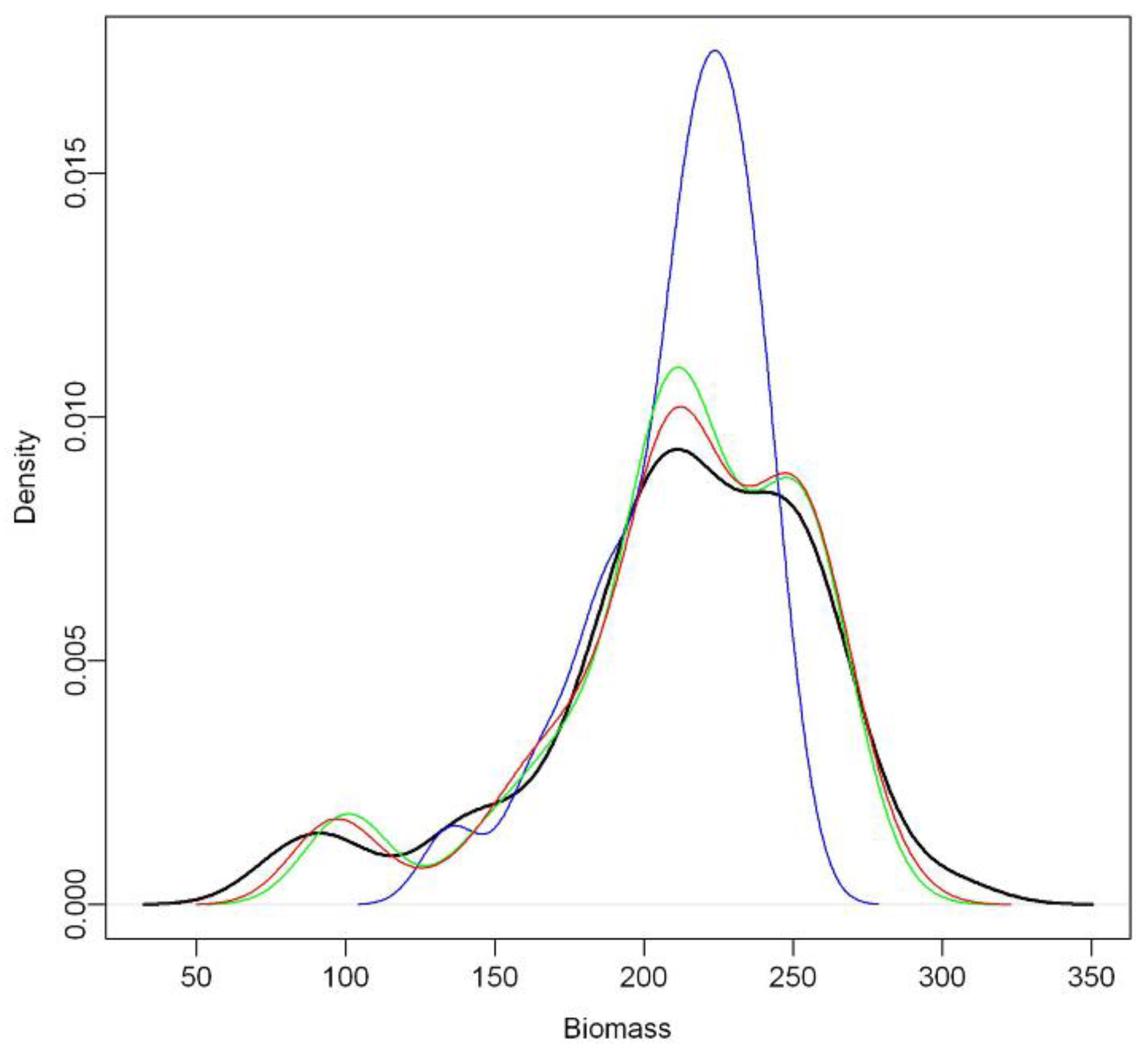
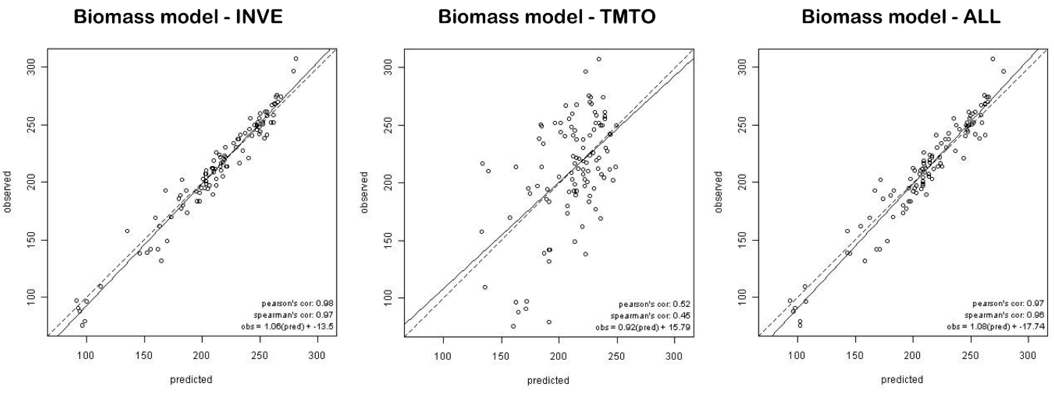
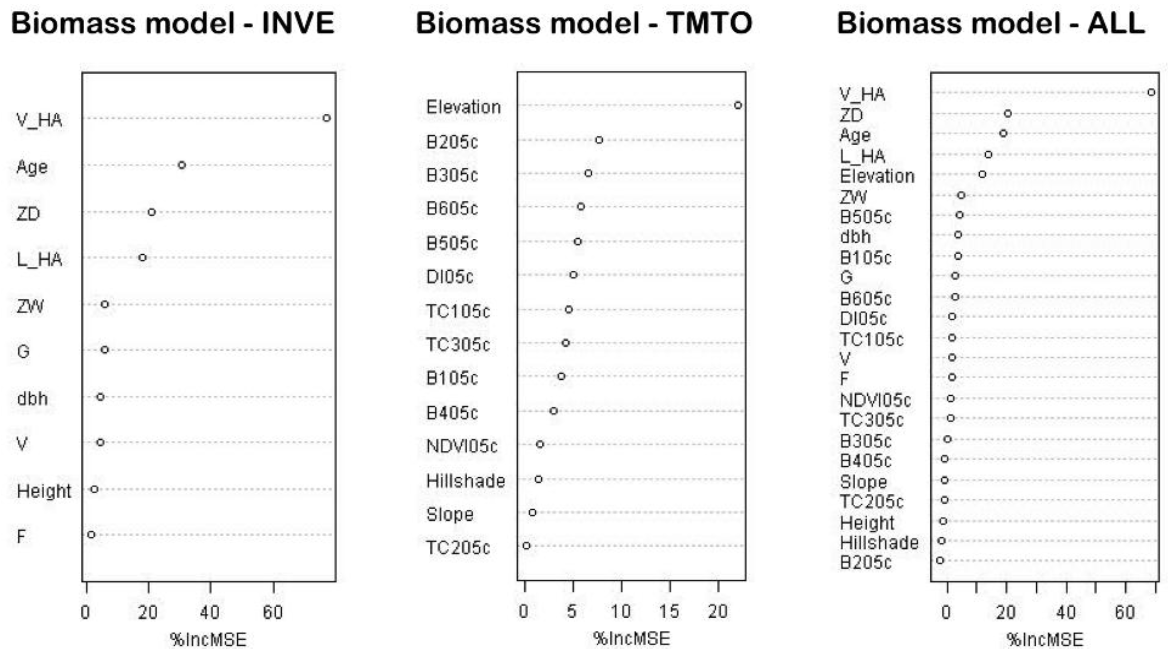
Our results showed a very strong relationship between inventory-based predictors and estimated biomass (Table 1). The INVE model was the most predictive for biomass, and captured the complete observed biomass range from approximately 100 to 300 Mg ha⁻¹ (Figure 3). These values are consistent with the typical range for boreal and temperate coniferous forests [15,52,53]. Using our modeling techniques for areas with up-to-date SBI, we found stand volume, relative density, and dominant tree age (Table 3) to be the strongest predictors for biomass estimation. This is consistent with allometric equations that often also incorporate these variables [15,17]. Generally, the predictive power of inventory-derived stand structure metrics is very high, especially for stand volume (Table 3).

Biomass estimates for areas lacking forest inventory data (TMTO) led to considerably less precise results. None of the pixel-based variables, aside from elevation, significantly contributed to biomass prediction. Powell et al. [36] also reported similar results based on Landsat data and in areas with strong elevational gradients. In our case, elevation often correlates with the forest dieback experienced during the past decade, which may explain its relationship to biomass distribution [40].

Tests on individual field-derived predictors which have improved TMTO-based biomass estimates (Table 4 and Table 5) provide promising results. We found that stand volume or even tree height—parameters easily taken in the field—significantly increased the correlation between observed and predicted biomass. Moreover, as tree height is easily measured in the field or can be measured from airborne Lidar data, we strongly recommend its inclusion to improve prediction results. To summarize, as might be expected, models based on SBI predicted biomass are better than models based on satellite data. However, by integrating TM data and stand volume or tree height information, our biomass estimate accuracy increased significantly. Our method therefore provides increased spatial detail within inventory polygons and fills the “knowledge gaps” in areas lacking SBI.

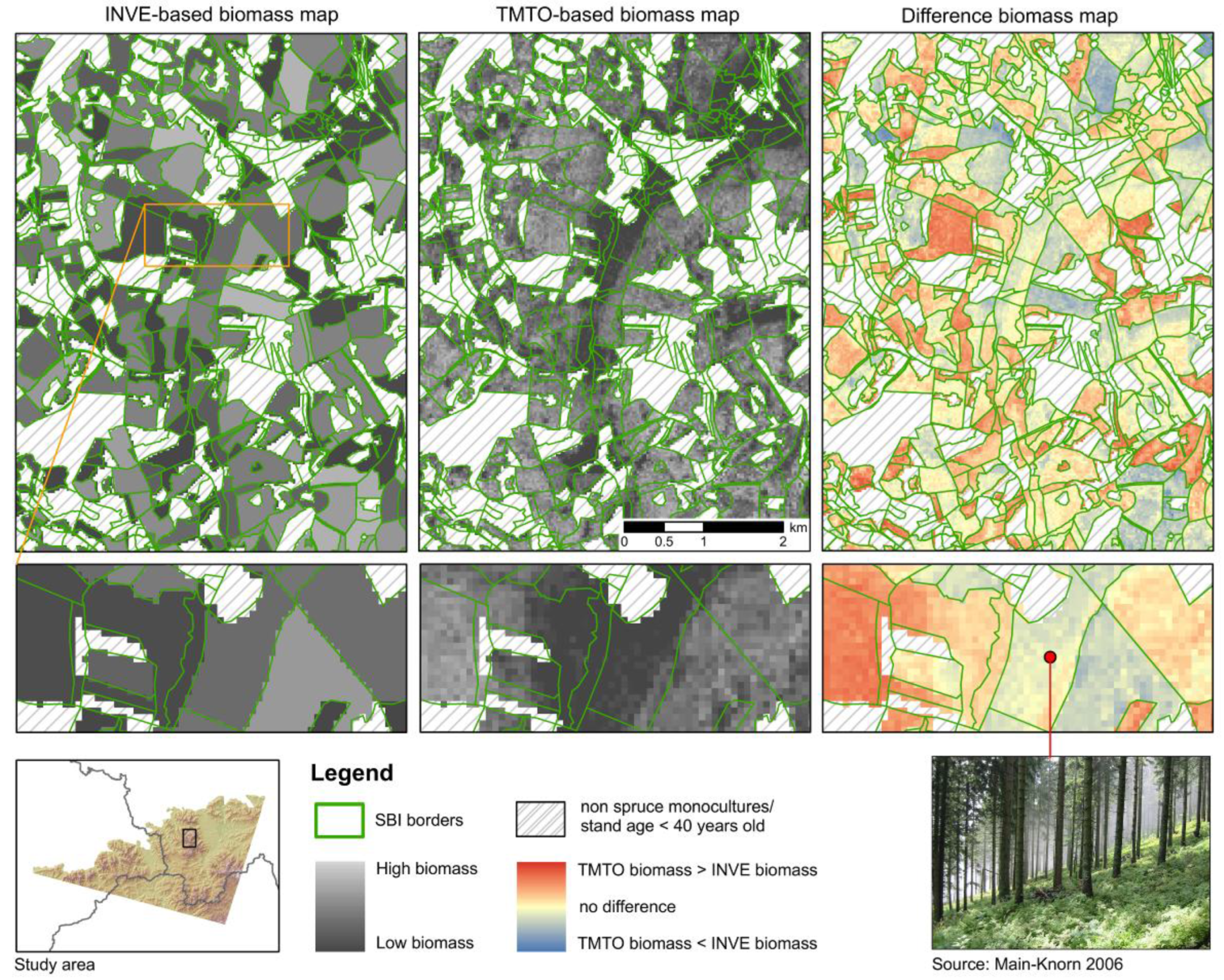
Beyond absolute model quality, we focused on the usefulness of remote sensing-based results in dealing with spatial variability within forest inventory stands. Our difference map highlights the potential of spectral data compared to polygon-based inventory layers that average stand-wise heterogeneity (Figure 6). Even in homogenous areas such as those selected for this study, it is obvious that remote sensing-based mapping results support decision-making at a sub-stand level and reveal spatial detail that would otherwise be averaged out. In addition, remote sensing-based estimates of forest stand parameters is more time-efficient; it rather depends on the research or management question at hand if accuracy trade-offs between field-based and remote sensing-based results may be more important than spatial or temporal detail.

TMTO-based estimates better represent short-term dynamics that often do not show up in biomass estimates from INVE-models. Long intervals between field-based inventories lead to mismatches between TMTO- and INVE-based biomass estimates. Differences are particularly obvious along forest stand borders, where, e.g., windbreak frequently caused great dynamics. Furthermore, the INVE-based biomass estimates for the whole southern part of the study area were overestimated compared to the satellite-based estimates. This is mainly related to temporal inconsistencies in the reference data (see Section 6.2).

Further differences between INVE- and TMTO-based biomass estimates relate to the spatial heterogeneity within forest stands. SBI-based estimates provide averaged biomass values for each stand, ignoring the spatial distribution of biomass and ecological complexity on the sub-stand level (Figure 6). Thus, stand-based inventory details may be sufficient to accomplish forest management tasks, while the same information may not be sufficient to describe temporal and spatial dynamics in forest ecosystems, e.g., related to carbon sequestration potential.

6.2. Innovation and Limitations

The availability of ground-truthed data and a homogeneous forest structure in our study site facilitated the evaluation of different models’ predictive power. Nevertheless, a few uncertainties remained. Firstly, different explanatory variables might not perfectly match each other due to temporal differences in our reference data. SBI data from different forest districts are collected independently of one another and consequently also in different years. The latest SBI data updates were available for 2003, 2004 and 2007 in the different districts, respectively. Thus, the extent of windbreak after the destructive storms in November 2004 and following sanitary cutting in 2005 might be missed in some of our district’s SBI. Similarly, Landsat data from early September 2005 might not reflect the total extent of sanitary clearcut measures. Thus, inevitable time shifts between SBI, Landsat data and field measurements (2006, 2007) do not reflect exactly the same forest situation.

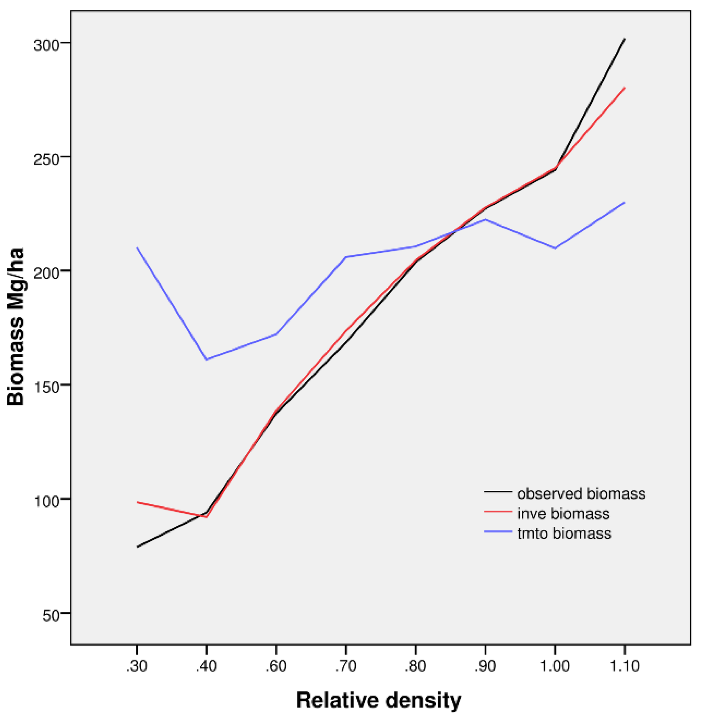
Secondly, the model estimates tend to bias for low and high target values. We found slight over- and under-estimates for lower and higher biomass values, respectively. The tendency to over-predict low biomass and under-predict high biomass conditions (Figure 3) has also been identified in previous studies, for instance where regression tree techniques [54] or kNN algorithms [55] were applied. This tendency is most likely related to two factors: optical sensors have a limited sensitivity for reproducing the canopy structure in dense forests, where biomass can lead to saturated measurements. There is also the confounding effect of understory vegetation in sparse and/or young forests, where forest biomass is generally low. We illustrated these effects in the example of AGB by comparing relative stand density with observed and predicted biomass values (Figure 7). AGB is highly positively correlated with relative density, as shown for observed biomass (reference) and INVE-based estimates. TMTO-based estimates revealed only a moderate relationship to stand density. Regarding dense forests, we observed considerable underestimates of TMTO-based biomass for relative forest densities above 0.9. Additionally, overestimated TMTO-based biomass values, as found in the case of low relative stand density and in the presence of understory as well as underwood, confirms their confounding effect in spectral data. Moreover, overestimation of biomass for spruce stands with tree age below 50 years may also be related to a low sample representation (about 3%) of young forest stands in the modeling process.

Figure 7. Relative stand density, observed biomass (black line) and predicted values of biomass for models INVE (red line) and TMTO (blue line) for all of 105 stands we sampled in summer 2006 and 2007.

Figure 7. Relative stand density, observed biomass (black line) and predicted values of biomass for models INVE (red line) and TMTO (blue line) for all of 105 stands we sampled in summer 2006 and 2007.

Thirdly, while spruce stands in our study area and Ukraine are very similar, differences due to regional climate variability and genetic origin exist. Minor inaccuracies in model parameterization and hence biomass estimates can therefore not be completely ruled out.

An integrated modeling approach combining SBI and satellite data has obvious advantages for determining spatial variability in forest biomass and structure. Our findings demonstrated that the integrated use of satellite data compliments stand level inventories, though the latter had the greater predictive strength for aboveground biomass if SBI information is updated regularly. Nevertheless, field-based information alone will, due to time- and work-intensive updating procedures, not deliver all the necessary information in such a dynamic region within a reasonable time frame.

Combining SBI and satellite data (ALL) did not improve the accuracy of biomass estimates. However, an integrated approach facilitates better detection of horizontal structural heterogeneity in forest systems [56], thereby guiding ground-based sampling intensity and distribution. In addition, it would not just reveal important information about mean carbon stocks, but also about the spatial distribution in stand structure and ecological complexity with which biomass is correlated (Figure 6). The capacity to map spatial co-variation among multiple ecosystem attributes has important implications for sustainable forest management and planning where the objective is to optimize the provision of multiple ecosystem services, including carbon storage, timber harvest, and biodiversity [57,58].

7. Conclusions

We modeled forest AGB estimates for spruce monocultures in the Western Carpathians using additional data sources, as suggested, for example, by Lu [14]. Where inventory data is available, it is an excellent source of spatial information regarding biomass in the Western Carpathians. However, in the case of missing, outdated or incomplete inventories, alternative approaches are needed. We elaborate on how to use spectral data to model biomass, thereby substituting or minimizing the need for inventory data. Our approach has been tested for vertically simple canopies as found, for example, in even-aged monocultures. Further research is needed to infer transferability to more complex or boreal conditions.

Based on Landsat and topography data alone, the AGB prediction model captured 27% of the biomass variability in the study area. However, including inventory-based stand volume, our modeling accuracies increased to 86%. Results suggest that spectral and topography data combined with selected inventory information provide highly accurate AGB estimates.

Our results encourage applications of biomass estimates to spruce forest stands across the entire Carpathian Mountain range. The next step, therefore, is to investigate the applicability of our findings to homogeneous spruce stands across this mountain range and beyond. This will require additional sensitivity analyses, e.g., concerning the influence of forest health status on modeling accuracy. There are several promising directions for further research. These include: (1) exploration of the influence of canopy structure and condition (e.g., tree vigor, defoliation, etc.) on biomass prediction; (2) assessment of how relationships between forest dieback, elevational gradients and understory reflectance might influence biomass modeling; and (3) research on the integration of TM data, and at least one selected inventory-based forest parameter for improving AGB modeling.

References

1. Bonan, G.B. Forests and climate change: Forcings, feedbacks, and the climate benefits of forests. Science 2008, 320, 1444–1449. [Google Scholar] [CrossRef] [PubMed]
2. Eggers, J.; Lindner, M.; Zudin, S.; Zaehle, S.; Lisk, J. Impact of changing wood demand, climate and land use on European forest resources and carbon stocks during the 21st century. Glob. Change Biol. 2008, 14, 2288–2303. [Google Scholar] [CrossRef]
3. Schulp, C.J.E.; Nabuurs, G.J.; Verburg, P.H. Future carbon sequestration in Europe—Effects of land use change. Agric. Ecosyst. Environ. 2008, 127, 251–264. [Google Scholar] [CrossRef]
4. Aber, J.; Neilson, R.P.; McNulty, S.; Lenihan, J.M.; Bachelet, D.; Drapek, R.J. Forest processes and global environmental change: Predicting the effects of individual and multiple stressors. Bioscience 2001, 51, 735–751. [Google Scholar] [CrossRef]
5. Ollinger, S.V.; Aber, J.D.; Reich, P.B.; Freuder, R.J. Interactive effects of nitrogen deposition, tropospheric ozone, elevated CO2 and land use history on the carbon dynamics of northern hardwood forests. Glob. Change Biol. 2002, 8, 545–562. [Google Scholar] [CrossRef]
6. Kuemmerle, T.; Olofsson, P.; Chaskovskyy, O.; Baumann, M.; Ostapowicz, K.; Woodcock, C.; Houghton, R.A.; Hostert, P.; Keeton, W.S.; Radeloff, V.C. Post-Soviet farmland abandonment, forest recovery, and carbon sequestration in western Ukraine. Glob. Change Biol. 2011, 17, 1335–1349. [Google Scholar] [CrossRef]
7. Running, S.W.; Gower, S.T. Forest-Bgc, a general-model of forest ecosystem processes for regional applications 2. Dynamic carbon allocation and nitrogen budgets. Tree Physiol. 1991, 9, 147–160. [Google Scholar] [CrossRef] [PubMed]
8. Cienciala, E.; Running, S.W.; Lindroth, A.; Grelle, A.; Ryan, M.G. Analysis of carbon and water fluxes from the NOPEX boreal forest: Comparison of measurements with FOREST-BGC simulations. J. Hydrol. 1998, 213, 62–78. [Google Scholar] [CrossRef]
9. Song, C.H.; Woodcock, C.E. A regional forest ecosystem carbon budget model: Impacts of forest age structure and landuse history. Ecol. Modell. 2003, 164, 33–47. [Google Scholar] [CrossRef]
10. Beer, C.; Reichstein, M.; Tomelleri, E.; Ciais, P.; Jung, M.; Carvalhais, N.; Rödenbeck, C.; Arain, M.A.; Baldocchi, D.; Bonan, G.B.; et al. Terrestrial gross carbon dioxide uptake: Global distribution and covariation with climate. Science 2010, 329, 834–838. [Google Scholar] [CrossRef] [PubMed]
11. Hall, F.G.; Shimabukuro, Y.E.; Huemmrich, K.F. Remote-sensing of forest biophysical structure using mixture decomposition and geometric reflectance models. Ecol. Appl. 1995, 5, 993–1013. [Google Scholar] [CrossRef]
12. Asner, G.P.; Scurlock, J.M.O.; Hicke, J.A. Global synthesis of leaf area index observations: Implications for ecological and remote sensing studies. Glob. Ecol. Biogeogr. 2003, 12, 191–205. [Google Scholar] [CrossRef]
13. Kutsch, W.L.; Liu, C.J.; Hormann, G.; Herbst, M. Spatial heterogeneity of ecosystem carbon fluxes in a broadleaved forest in Northern Germany. Glob. Change Biol. 2005, 11, 70–88. [Google Scholar] [CrossRef]
14. Lu, D. The potential and challenge of remote sensing-based biomass estimation. Int. J. Remote Sens. 2006, 27, 1297–1328. [Google Scholar] [CrossRef]
15. Wulder, M.A.; White, J.C.; Fournier, R.A.; Luther, J.E.; Magnussen, S. Spatially explicit large area biomass estimation: Three approaches using forest inventory and remotely sensed imagery in a GIS. Sensors 2008, 8, 529–560. [Google Scholar] [CrossRef]
16. Jenkins, J.C.; Chojnacky, D.C.; Heath, L.S.; Birdsey, R.A. National-scale biomass estimators for United States tree species. Forest Sci. 2003, 49, 12–35. [Google Scholar]
17. Lakida, P.; Nilsson, S.; Shvidenko, A. Estimation of forest phytomass for selected countries of the former European USSR. Biomass Bioenergy 1996, 11, 371–382. [Google Scholar] [CrossRef]
18. Zianis, D.; Muukkonen, P.; Mäkipää, R.; Mencuccini, M. Biomass and stem volume equations for tree species in Europe. Silva Fennica Monographs 2005, 4, 1–63. [Google Scholar]
19. Luther, J.E.; Fournier, R.A.; Piercey, D.E.; Guindon, L.; Hall, R.J. Biomass mapping using forest type and structure derived from Landsat TM imagery. Int. J. Appl. Earth Obs. Geoinf. 2006, 8, 173–187. [Google Scholar] [CrossRef]
20. Nilson, T.; Anniste, J.; Lang, M.; Praks, J. Determination of needle area indices of coniferous forest canopies in the NOPEX region by ground-based optical measurements and satellite images. Agric. Forest Meteorol. 1999, 98–99, 449–462. [Google Scholar]
21. Chen, J.M.; Pavlic, G.; Brown, L.; Cihlar, J.; Leblanc, S.G.; White, H.P.; Hall, R.J.; Peddle, D.R.; King, D.J.; Trofymow, J.A.; et al. Derivation and validation of Canada-wide coarse-resolution leaf area index maps using high-resolution satellite imagery and ground measurements. Remote Sens. Environ. 2002, 80, 165–184. [Google Scholar] [CrossRef]
22. Shvidenko, A.; Schepaschenko, D.; Nilsson, S.; Bouloui, Y. Semi-empirical models for assessing biological productivity of Northern Eurasian forests. Ecol. Model. 2007, 204, 163–179. [Google Scholar] [CrossRef]
23. Wu, Y.C.; Strahler, A.H. Remote estimation of crown size, stand density, and biomass on the Oregon transect. Ecol. Appl. 1994, 4, 299–312. [Google Scholar] [CrossRef]
24. Peddle, D.R.; Hall, F.G.; LeDrew, E.F. Spectral mixture analysis and geometric-optical reflectance modeling of boreal forest biophysical structure. Remote Sens. Environ. 1999, 67, 288–297. [Google Scholar] [CrossRef]
25. Eklundh, L.; Harrie, L.; Kuusk, A. Investigating relationships between Landsat ETM plus sensor data and leaf area index in a boreal conifer forest. Remote Sens. Environ. 2001, 78, 239–251. [Google Scholar] [CrossRef]
26. De Veaux, R.D. A Guided Tour of Modern Regression Methods. In Proceedings of 1995 Fall Technical Conference, Section on Physical and Engineering Sciences, St. Louis, MO, USA, 19–20 October 1995.
27. Moisen, G.G.; Frescino, T.S. Comparing five modelling techniques for predicting forest characteristics. Ecol. Model. 2002, 157, 209–225. [Google Scholar] [CrossRef]
28. Breiman, L. Random forests. Mach. Learn. 2001, 45, 5–32. [Google Scholar] [CrossRef]
29. Morgan, J.N.; Sonquist, J.A. Problems in analysis of survey data, and a proposal. J. Am. Stat. Assoc. 1963, 58, 415–434. [Google Scholar] [CrossRef]
30. Breiman, L.; Friedman, J.H.; Olshen, R.A.; Stone, C.J. Classification and Regression Trees; Chapman & Hall: Monterey, CA, USA, 1984; p. 358. [Google Scholar]
31. Liaw, A.; Wiener, M. Classification and regression by randomForest. R News 2002, 2, 18–22. [Google Scholar]
32. Cutler, D.R.; Edwards, T.C.; Beard, K.H.; Cutler, A.; Hess, K.T.; Gibson, J.; Lawler, J.J. Random forests for classification in ecology. Ecology 2007, 88, 2783–2792. [Google Scholar] [CrossRef] [PubMed]
33. Prasad, A.M.; Iverson, L.R.; Liaw, A. Newer classification and regression tree techniques: Bagging and random forests for ecological prediction. Ecosystems 2006, 9, 181–199. [Google Scholar] [CrossRef]
34. Francke, T.; Lopez-Tarazon, J.A.; Schroder, B. Estimation of suspended sediment concentration and yield using linear models, random forests and quantile regression forests. Hydrol. Process. 2008, 22, 4892–4904. [Google Scholar] [CrossRef]
35. Falkowski, M.J.; Evans, J.S.; Martinuzzi, S.; Gessler, P.E.; Hudak, A.T. Characterizing forest succession with lidar data: An evaluation for the Inland Northwest, USA. Remote Sens. Environ. 2009, 113, 946–956. [Google Scholar] [CrossRef]
36. Powell, S.L.; Cohen, W.B.; Healey, S.P.; Kennedy, R.E.; Moisen, G.G.; Pierce, K.B.; Ohmann, J.L. Quantification of live aboveground forest biomass dynamics with Landsat time-series and field inventory data: A comparison of empirical modeling approaches. Remote Sens. Environ. 2010, 114, 1053–1068. [Google Scholar] [CrossRef]
37. Kozak, J. Przestrzenny model degradacji lasów Beskidu Śląskiego. Biuletyn KPZK 1996, 174, 511–538. [Google Scholar]
38. Bytnerowicz, A.; Badea, O.; Barbu, I.; Fleischer, P.; Fraczek, W.; Gancz, V.; Godzik, B.; Grodzinska, K.; Grodzki, W.; Karnosky, D.; et al. New international long-term ecological research on air pollution effects on the Carpathian Mountain forests, Central Europe. Environ. Int. 2003, 29, 367–376. [Google Scholar] [CrossRef]
39. Grodzki, W. Threats to the mountain norway spruce stands in the Carpathians from the insect pests. In Current Problems of Forest Protection in Spruce Stands under Conversion; Grodzki, W., Oszako, T., Eds.; IBL, Forest Research Institute (FRI): Warsaw, Poland, 2006; pp. 71–78. [Google Scholar]
40. Main-Knorn, M.; Hostert, P.; Kozak, J.; Kuemmerle, T. How pollution legacies and land use histories shape post-communist forest cover trends in the Western Carpathians. Forest Ecol. Manag. 2009, 258, 60–70. [Google Scholar] [CrossRef]
41. Fabijanowski, J.; Jaworski, A. Gospodarstwo leśne (Silviculture). In Karpaty Polskie—Przyroda, Człowiek i jego działalność (The Polish Carpathians—Nature, Man and His Activities); Warszyńska, J., Ed.; Uniwersytet Jagielloński w Krakowie: Kraków, Poland, 1995; pp. 253–263. [Google Scholar]
42. Ditmarová, L.; Kmeť, J.; Ježík, M.; Váľka, J. Mineral nutrition in relation to the Norway spruce forest decline in the region Horný Spiš (Northern Slovakia). J. Forest Sci. 2007, 53, 93–100. [Google Scholar]
43. Grodzki, W. Spatio-temporal patterns of the Norway spruce decline in the Beskid Śląski and Żywiecki (Western Carpathians) in southern Poland. J. Forest Sci. 2007, 53, 38–44. [Google Scholar]
44. Šrámek, V.; Vejpustková, M.; Novotný, R.; Hellebrandová, K. Yellowing of Norway spruce stands in the Silesian Beskids—Damage extent and dynamics. J. Forest Sci. 2008, 54, 55–63. [Google Scholar]
45. Slater, J.A.; Garvey, G.; Johnston, C.; Haase, J.; Heady, B.; Kroenung, G.; Little, J. The SRTM data “finishing” process and products. Photogramm. Eng. Remote Sensing 2006, 72, 237–247. [Google Scholar] [CrossRef]
46. Hill, J.; Mehl, W. Geo- and radiometric pre-processing of multi- and hyper-spectral data for the production of calibrated multi-annual time series. Photogrammetrie-Fernerkundung-Geoinformation (PFG) 2003, 7, 7–14. [Google Scholar]
47. Tanré, D.; Deroo, C.; Duhaut, P.; Herman, M.; Morcrette, J.J.; Perbos, J.; Deschamps, P.Y. Description of a computer code to simulate the satellite signal in the solar spectrum—The 5S Code. Int. J. Remote Sens. 1990, 11, 659–668. [Google Scholar] [CrossRef]
48. IPCC. Good Practice Guidance for Land Use, Land-Use Change and Forestry; Institute for Global Environmental Strategies (IGES): Hayama, Japan, 2003. [Google Scholar]
49. Healey, S.P.; Cohen, W.B.; Yang, Z.Q.; Krankina, O.N. Comparison of Tasseled Cap-based Landsat data structures for use in forest disturbance detection. Remote Sens. Environ. 2005, 97, 301–310. [Google Scholar] [CrossRef]
50. Rehfeldt, G.E.; Crookston, N.L.; Warwell, M.V.; Evans, J.S. Empirical analyses of plant-climate relationships for the western United States. Int. J. Plant Sci. 2006, 167, 1123–1150. [Google Scholar] [CrossRef]
51. Marmion, M.; Luoto, M.; Heikkinen, R.K.; Thuiller, W. The performance of state-of-the-art modelling techniques depends on geographical distribution of species. Ecol. Model. 2009, 220, 3512–3520. [Google Scholar] [CrossRef]
52. Fehrmann, L.; Kleinn, C. General considerations about the use of allometric equations for biomass estimation on the example of Norway spruce in central Europe. Forest Ecol. Manag. 2006, 236, 412–421. [Google Scholar] [CrossRef]
53. Keeton, W.S.; Chernyavskyy, M.; Gratzer, G.; Main-Knorn, M.; Shpylchak, M.; Bihun, Y. Structural characteristics and aboveground biomass of old-growth spruce-fir stands in the eastern Carpathian mountains, Ukraine. Plant Biosyst. 2010, 144, 148–159. [Google Scholar] [CrossRef]
54. Blackard, J.A.; Finco, M.V.; Helmer, E.H.; Holden, G.R.; Hoppus, M.L.; Jacobs, D.M.; Lister, A.J.; Moisen, G.G.; Nelson, M.D.; Riemann, R.; et al. Mapping US forest biomass using nationwide forest inventory data and moderate resolution information. Remote Sens. Environ. 2008, 112, 1658–1677. [Google Scholar] [CrossRef]
55. Reese, H.; Nilsson, M.; Sandström, P.; Olsson, H. Applications using estimates of forest parameters derived from satellite and forest inventory data. Comput. Electron. Agric. 2002, 37, 37–55. [Google Scholar] [CrossRef]
56. Franklin, J.F.; Spies, T.A.; Van Pelt, R.; Carey, A.B.; Thornburgh, D.A.; Berg, D.R.; Lindenmayer, D.B.; Harmon, M.E.; Keeton, W.S.; Shaw, D.C.; et al. Disturbances and structural development of natural forest ecosystems with silvicultural implications, using Douglas-fir forests as an example. Forest Ecol. Manag. 2002, 155, 399–423. [Google Scholar] [CrossRef]
57. Keeton, W.S. Role of managed forestlands and models for sustainable forest management: perspectives from North America. George Wright Forum 2007, 24, 38–53. [Google Scholar]
58. Wolfslehner, B.; Seidl, R. Harnessing ecosystem models and multi-criteria decision analysis for the support of forest management. Environ. Manag. 2010, 46, 850–861. [Google Scholar] [CrossRef] [PubMed]