Article

Effect of Reduced Spatial Resolution on Mineral Mapping Using Imaging Spectrometry—Examples Using Hyperspectral Infrared Imager (HyspIRI)-Simulated Data

by
Fred A. Kruse
1,2,*,
James V. Taranik
2,
Mark Coolbaugh
2,3,
Joshua Michaels
2,
Elizabeth F. Littlefield
2,
Wendy M. Calvin
2 and
Brigette A. Martini
4
1
Physics Department and Remote Sensing Center, Naval Postgraduate School, 833 Dyer Rd., Monterey, CA 93943, USA
2
Department of Geological Sciences and Engineering and Arthur Brant Laboratory for Exploration Geophysics, University of Nevada, MS 172, 1664 N. Virginia St., Reno, NV 89557, USA
3
Renaissance Gold, Inc., 4750 Longley Lane, Suite 106, Reno, NV 89502, USA
4
Ormat Nevada Inc., 6225 Neil Rd., Reno, NV 89557, USA
*
Author to whom correspondence should be addressed.
Remote Sens. 2011, 3(8), 1584-1602; https://doi.org/10.3390/rs3081584
Submission received: 6 June 2011 / Revised: 2 July 2011 / Accepted: 14 July 2011 / Published: 25 July 2011
(This article belongs to the Special Issue Hyperspectral Remote Sensing)

Abstract

:
The Hyperspectral Infrared Imager (HyspIRI) is a proposed NASA satellite remote sensing system combining a visible to shortwave infrared (VSWIR) imaging spectrometer with over 200 spectral bands between 0.38 and 2.5 μm and an 8-band thermal infrared (TIR) multispectral imager, both at 60 m spatial resolution. Short Wave Infrared (SWIR) (2.0–2.5 μm) simulation results are described here using Airborne Visible/Infrared Imaging Spectrometer (AVIRIS) data in preparation for the future launch. The simulated data were used to assess the effect of the HyspIRI 60 m spatial resolution on the ability to identify and map minerals at hydrothermally altered and geothermal areas. Mineral maps produced using these data successfully detected and mapped a wide variety of characteristic minerals, including jarosite, alunite, kaolinite, dickite, muscovite-illite, montmorillonite, pyrophyllite, calcite, buddingtonite, and hydrothermal silica. Confusion matrix analysis of the datasets showed overall classification accuracy ranging from 70 to 92% for the 60 m HyspIRI simulated data relative to 15 m spatial resolution data. Classification accuracy was lower for similar minerals and smaller areas, which were not mapped well by the simulated 60 m HyspIRI data due to blending of similar signatures and spectral mixing with adjacent pixels. The simulations demonstrate that HyspIRI SWIR data, while somewhat limited by their relatively coarse spatial resolution, should still be useful for mapping hydrothermal/geothermal systems, and for many other geologic applications requiring mineral mapping.

1. Introduction

Imaging spectrometry, the simultaneous measurement of continuous spectra and images in up to hundreds of spectral channels or bands, is a proven technology for identifying and mapping materials based on their spectral signatures [1,2]. It has also become known as “Hyperspectral Imaging” or “HSI”. Spectral mapping using imaging spectrometer data is well established and routinely used for numerous applications [3,4,5,6,7,8,9]. Probably the most widely documented use of these data is for identifying and mapping specific minerals associated with hydrothermally altered rocks (rocks changed by hot water moving through them), which occur in active geothermal systems and relict mineralized systems (ore deposits) worldwide [1,9,10,11,12,13,14].
The Hyperspectral Infrared Imager (HyspIRI) is a proposed NASA satellite remote sensing system combining a visible to shortwave infrared (VSWIR) imaging spectrometer with over 200 spectral bands between 0.38–2.5 μm and an 8-band thermal infrared (TIR) multispectral imager [15]. The TIR system will have a single mid-wave infrared (MWIR) band at approximately 4 μm and seven spectral bands in the long-wave infrared (LWIR) between 7.3 and 12.1 μm. While HyspIRI is principally designed for ecosystem applications [15], it is expected that the system will have significant geologic capabilities as well [16]. Another hyperspectral instrument (Hyperion) has already demonstrated that mineral mapping from space is viable at 30 m spatial resolution, albeit with signal-to-noise (SNR) limitations that resulted in reduced capabilities comparable to airborne systems [11].
In preparation for HyspIRI, we have generated and analyzed simulated datasets using existing NASA imaging spectrometer data and multispectral airborne data to demonstrate HyspIRI’s suitability and potential for mineral mapping from space. The Airborne Visible/Infrared Imaging Spectrometer (AVIRIS) [17,18,19,20] at approximately 15 m spatial resolution was used to simulate the HyspIRI VSWIR data at 10 nm spectral resolution and 60 m spatial resolution. The MODIS/ASTER airborne simulator (MASTER) or MODIS airborne simulator (MAS) sensors, with 10 and 6 spectral bands respectively in the 8–14 μm range, provided the data for the MWIR band and the seven HyspIRI-simulated LWIR spectral bands. Only the SWIR mineral mapping utilizing the 2.0–2.5 μm region are described here.

2. Approach and Methods

The airborne datasets were geocorrected and coregistered to construct the full simulated VSWIR-TIR HyspIRI datasets using orthorectified Advanced Spaceborne Thermal Emission and Reflection Spectrometer (ASTER) data [21] as a geographic base. For the SWIR, AVIRIS data were converted to apparent reflectance using “ACORN”, a MODTRAN atmospheric-model-based radiance to reflectance correction [22,23] and spectrally resampled using the proposed HyspIRI 10 nm spectral resolution [15,20]. They were then spatially registered to the orthorectified ASTER data using ground control points (GCPs), Delaunay Triangulation, and Nearest Neighbor resampling. Spatial resampling of the 15 m data to the 60 m HyspIRI spatial resolution was accomplished using pixel aggregation (pixel averaging). The 60 m spatial resolution simulated-HyspIRI data were finally resized to the same image size as the 15 m geocorrected data using integer pixel replication to allow direct digital comparison of the two spatial resolutions. No attempt was made to simulate HyspIRI SNR response, as the proposed HyspIRI response of approximately 400:1 in the SWIR is substantially similar to the performance of AVIRIS datasets used for these simulations (~400:1 or better in the SWIR for 1995 onward) [18,20]. The results described here assume that HyspIRI SNR projections will be met.
A standardized analysis approach was used on each dataset to extract a few diagnostic image spectra and map their spatial locations [24]. This consists of reduction of the spectral dimensions using the Minimum Noise Fraction (MNF) Transformation [25,26], spatial reduction using the Pixel Purity Index (PPI) [27], and n-Dimensional scatterplotting to extract “endmembers” [28]. Endmembers consist of those spectra that can be combined in a linear mixing fashion to explain every spectral signature in the data. Mineral mapping matches these spectra to every pixel spectrum, estimating their abundances, and validating that the result is a valid mixture of the desired spectrum and the background (MTMF) [29]. The results are presented as color-coded image maps of the most abundant mineral per pixel. While multiple minerals do occur at many pixels (as mixtures), only the simplified mineral maps are shown here for comparison of 15 m versus 60 m mineral mapping.

3. Results and Discussion

Our HyspIRI simulations span a variety of sites—both active geothermal and fossil hydrothermal systems. These include hydrothermal alteration at Cuprite, Nevada and Fish Lake Valley, Nevada; and geothermal systems at Steamboat Springs, Nevada, Long Valley, California, and Yellowstone National Park, Wyoming. We summarize selected results for Cuprite, Nevada; Steamboat Springs, Nevada; and Yellowstone, Wyoming here.

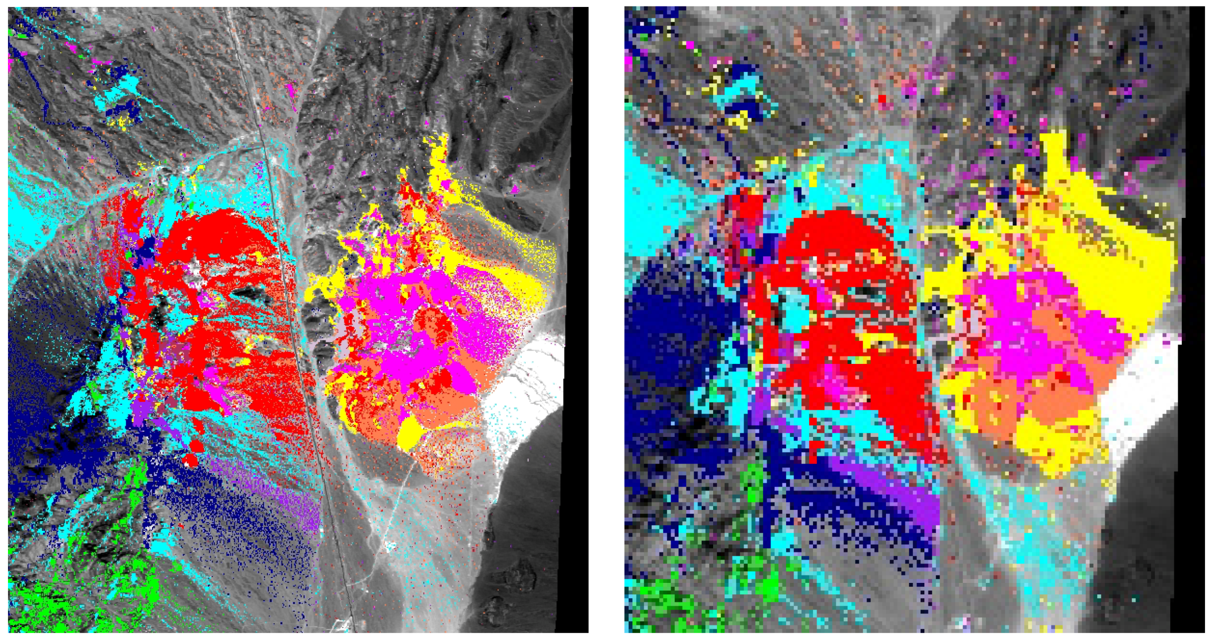
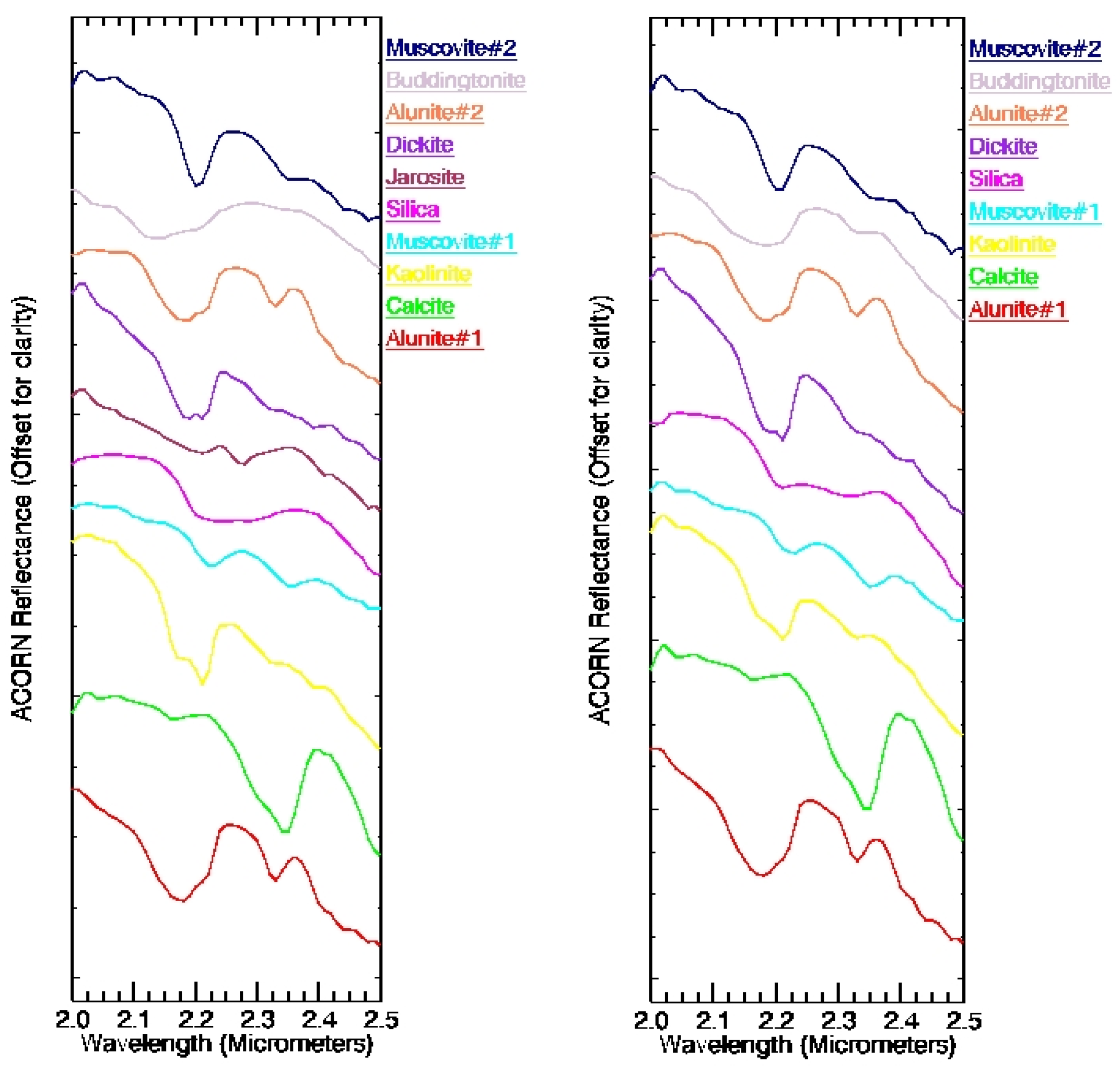
3.1. Cuprite, NV, Site (Fossil Hydrothermal System)

The Cuprite mining district is located approximately 65 km (40 mi) south of Tonopah, Nevada. It consists of two spatially and temporally separate low-sulfur epithermal acid-sulfate systems separated by US Highway 95 [30]. Host rocks include Tertiary-age volcanic ash flow/air fall tuffs, flows, sedimentary conglomerates and sandstones and Cambrian-age carbonates, quartzites, siltstones (west side only). Abrams et al. [31] mapped three alteration zones (1) Argillized (kaolinite and/or montmorillonite); (2) Opalized (opal, variable alunite and kaolinite); and (3) Silicified (hydrothermal quartz ± calcite).
Cuprite AVIRIS data collected 20 September 2006 at approximately 15 m spatial resolution were atmospherically corrected to reflectance, spectrally resampled to the HyspIRI wavelength response, geocorrected to ASTER data at 15 m resolution, and spatially resampled to 60 m as described above. Visual comparisons were made between the original AVIRIS data and the 15 m spectrally resampled HyspIRI-simulated data of spectral signatures from areas of known composition and there were no discernable spectral differences. Endmember spectra were then extracted from the HyspIRI-simulated imaging spectrometer data at 15 m and 60 m spatial resolution using the MNF, PPI, n-D Visualizer approach. Extracted mineral spectra were compared with a spectral library developed by the USGS [32] for identification of minerals. The endmember spectra shown in Figure 1 are typical for those seen in epithermal ore deposits, representative of a fossilized hydrothermal system. These include kaolinite, dickite, alunite, buddingtonite, muscovite-illite, and hydrothermal silica. The calcite signatures are typical of those seen in unaltered limestones. Note the small differences between the 15 m and 60 m endmembers in Figure 1, caused by spectral mixing in the 60 m endmembers. The 15 m SWIR endmembers were used to perform mixture-tuned-matched-filtering (MTMF) mapping of the spectrally predominant mineral for each pixel in both the 15 m and 60 m HyspIRI-simulated data. The same matched filter (MF) cutoffs and MF/Infeasibility ratios were used to produce both images. Mapping at both resolutions resulted in visually similar mineral maps (the 15 m simulation is essentially identical to native AVIRIS data and results—not shown). The main difference is that some of the areas of specific minerals in the 15 m data are not present (or reduced in size) in the 60 m data because of dilution of pixel signatures by spectral mixing (Figure 2 and Figure 3).
Figure 1. Left: SWIR endmembers for the full Cuprite-Goldfield HyspIRI 15 m simulated dataset. Right: SWIR endmembers for the full Cuprite-Goldfield dataset at HyspIRI 60 m spatial resolution. There are some small differences between the endmember spectra caused by spectral mixing at the 60 m resolution. Most apparent of these in the 60 m resolution data are (1) a shift of the main feature for “buddingtonite” towards 2.16 μm caused by mixing with alunite; (2) shallowing of the 2.16 μm band for “dickite” to appear more similar to kaolinite; (3) disappearance of the jarosite endmember at 60 m resolution; (4) contamination of the broad 2.25 silica feature with other smaller features near 2.3 μm; and (5) loss of sharpness of the kaolinite doublet at 2.16 and 2.2 μm.
Remotesensing 03 01584 g001
Figure 2. Left: SWIR mineral map for the full Cuprite-Goldfield 15 m spatial resolution scene generated from Airborne Visible/Infrared Imaging Spectrometer (AVIRIS) data by geocorrecting to ASTER and spectrally resampling to HyspIRI spectrally response. Right: SWIR mineral map for the full Cuprite-Goldfield HyspIRI 60 m simulated dataset.
Remotesensing 03 01584 g002
Figure 3. Left: Zoomed portion of the 15 m spatial mineral map over the Cuprite Mining District. Endmember spectra used and colors match Figure 1 (Left). Image base is approximately 10 km, north is to the top. Right: Zoomed portion of the 60 m HyspIRI-simulated mineral map over the Cuprite Mining District. Endmember spectra used and colors match Figure 1 (Left). Image base is approximately 10 km, north is to the top.
Remotesensing 03 01584 g003
Accuracy assessment comparing the capability of the 60 m HyspIRI-simulated SWIR data to map the specific minerals identified at Cuprite, Nevada, as compared to the 15 m HyspIRI spectrally resampled data was conducted using a confusion matrix approach [33] for the subset shown in Figure 3. The SWIR mineral mapping results shown in Figure 3 were directly compared on a pixel-by-pixel basis using the 15 m mineral map as the “ground truth” (Table 1).
Overall accuracy of the 60 m classification as compared to the 15 m classification is estimated at approximately 81%. The calculated Kappa Coefficient, however, which assesses classification performance relative to chance, is only 0.46, falling into the generally accepted “Fair Agreement” category for the Kappa Coefficient statistic [34,35]. An examination of the diagonals of the confusion matrix shows accuracies ranging from approximately 24–85%. The best match is for kaolinite (however, see note about errors of commission below), while the worst match is for buddingtonite. It appears that most of the errors are probably attributable to spectral mixing as indicated by classification problems between similar minerals (e.g., kaolinite, dickite, and alunite; two types of alunite; two types of muscovite). The low score for buddingtonite is also probably caused by spectral mixing, as the buddingtonite exposures are typically small, and while well-resolved at 15 m spatial resolution 60 m HyspIRI-simulated pixels likely contain multiple minerals. The confusion matrix further shows that the there is a fairly even split of errors of commission versus omission, though errors for certain minerals (kaolinite, muscovite#2) are dominated by errors of commission. The producer accuracy (probability that the classifier has correctly labeled a pixel as a specific mineral given that the ground truth image pixel is that mineral) validate that HyspIRI should be able to map mineralogy at 60 m spatial resolution. The user accuracy (probability that the specific mineral has been correctly mapped given that the pixel has been classified as a specific mineral) is significantly lower for several of the minerals (e.g., kaolinite, muscovite#1, alunite#2, buddingtonite), again indicating confusion at 60 m resolution between similar minerals caused by spectral mixing. It does appear from the classification images (Figure 2 and Figure 3) and the confusion matrix (Table 1) that the HyspIRI sensor would do a reasonably good job of mapping the spatial distribution of hydrothermal alteration at the Cuprite, Nevada site. There is some loss of detail at the 60 m scale compared to the 15 m scale, however, the overall mineralogy and patterns are preserved and the simulated HyspIRI data can be used to generate a system model.
Table 1. Confusion matrix for Cuprite, Nevada, 15 m versus 60 m HyspIRI simulation. Overall Accuracy = (1533947/1905364) 80.5068%. Kappa Coefficient = 0.4627.
GroundTruth
ClassUnclassAlun#1CalciteKaoliniteMusc#1SilicaDickiteAlun#2Budding.Musc#2Total
Unclass84.0116.5224.995.8332.6411.2522.8542.7451.7419.2274.82
Alun#10.5263.830.020.911.070.442.718.212.540.211.98
Calcite0.630.0266.580.010.550.090.090.020.560.351.80
Kaolinite2.423.360.2284.842.8511.505.0310.534.010.933.58
Musc#14.202.425.630.7357.251.783.561.759.350.446.19
Silica0.890.220.140.130.3467.630.142.411.520.281.53
Dickite0.451.670.004.210.510.0153.930.160.140.720.86
Alun#21.359.030.051.160.646.500.3232.470.840.192.08
Budding.0.090.510.060.290.160.010.060.2124.110.040.16
Musc#25.432.422.311.903.990.7911.311.495.2077.627.01
Total100.00100.00100.00100.00100.00100.00100.00100.00100.00100.00100.00
ClassCommissionOmissionProd. Acc.User Acc.
PercentPercentPercentPercent
Unclass5.2815.9784.0394.72
Alun#134.9136.1763.8365.09
Calcite31.2733.4266.5868.73
Kaol73.2415.1684.8426.76
Musc#161.5642.7557.2538.44
Silica54.5932.3767.6345.41
Dickite58.4246.0753.9341.58
Alun#269.2267.5332.4730.78
Budding.65.2175.8924.1134.79
Musc#271.0822.3877.6228.92

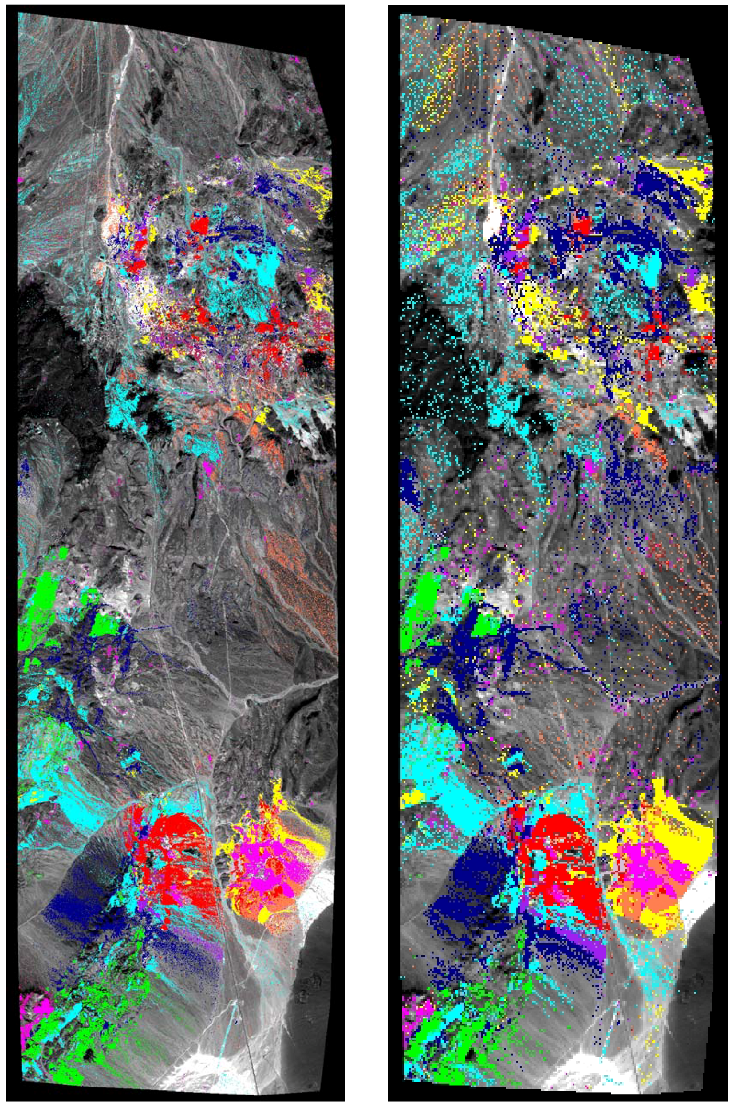
3.2. Steamboat, NV, Site (Active Geothermal System)

The Steamboat Springs hydrothermal system is described as a present-day equivalent of epithermal gold-silver deposits [36,37]. This geothermal system, located just south of Reno, Nevada is associated with four rhyolite domes. Thermal activity may be as old as 1.1 Ma, and has probably been continuous for at least the past 0.1 m.y [38]. Numerous wells have been drilled at Steamboat for geothermal energy and to obtain hot water for local resort facilities. The principal surface mineralogy at Steamboat consists of chalcedonic sinter deposits. Until approximately 1988, dark siliceous muds were also being deposited in the active springs and acid-leached opaline residues. Geothermal production has resulted in a drop in the water levels and subsequent cessation of surface deposition. Kaolinite, and alunite occur in solfatarically altered granodiorite and basaltic andesite in the western part of the area [39,40,41,42,43]. Significant concentrations of precious metals and related pathfinder elements occur in the Steamboat Springs sinter deposits, as chemical sediments in spring vents, and as veins at depth [44]. Gold was detected at the 1–2 ppm level along with anomalous Ag and As concentrations in analysis of samples from several drill holes, and small amounts of Hg has been mined from a mercury mine at Steamboat [45]. Deep drilling at Steamboat shows vein and alteration patterns that are indistinguishable from those of many epithermal ore deposits, containing adularia, illite, montmorillonite, and chlorite-group minerals as well as kaolinite, chalcedony, calcite, and quartz. Both stibnite and cinnabar are present near the surface, however, ore-grade concentrations of metals appear to be absent both in the near surface deposits and in the veins at depth. The Steamboat site currently produces approximately 100 megawatts of electricity from several geothermal power plants. Extensive hydrothermal alteration, and fumaroles and hot ground still present at a number of locations have been mapped by the authors using airborne VSWIR and TIR sensors [46,47,48] and digital temperature probes on the ground (Coolbaugh, unpublished data, 2006).
AVIRIS data acquired 22 July 1995 at approximately 15 m spatial resolution were atmospherically corrected to reflectance, spectrally resampled to HyspIRI spectral resolution, geocorrected to orthorectified ASTER data, and spatially resampled to 60 m resolution as previously described. Endmember spectra were extracted from the Steamboat Springs, NV HyspIRI-simulated imaging spectrometer data at 15 m spatial resolution, again using the MNF, PPI, n-D Visualizer approach described above [24]. Extracted 15 m mineral spectra were compared with the USGS spectral library for identification of minerals. The endmember spectra shown in Figure 4 (Left) are typical for those seen in both epithermal ore deposits (representative of a fossilized hydrothermal system) and in active geothermal systems. These include kaolinite, alunite, muscovite-illite, and hydrothermal silica (Figure 4, Left). Pyrophyllite is also seen in an area outside the Steamboat Springs system. The 15 m SWIR endmembers were used to perform mixture-tuned-matched-filtering (MTMF) mapping of the spectrally predominant mineral for each pixel in both the 15 m and 60 m HyspIRI-simulated data (Figure 4, Right). The same matched filter (MF) cutoffs and MF/Infeasibility ratios were used to produce both images. Mapping at both resolutions resulted in visually similar mineral maps). Similar to Cuprite, but more dramatic because of some of the smaller mineral exposures, the main difference is that some of the areas of specific minerals in the 15 m data are not present (or reduced in size) in the 60 m data, because of dilution of pixel signatures by spectral mixing (Figure 4, Right).
Accuracy assessment was also performed for the Steamboat, Nevada 60 m simulated HyspIRI data, comparing the capability to map specific minerals with respect to the 15 m HyspIRI spectrally resampled data using the confusion matrix approach [33]. The SWIR mineral mapping results shown in Figure 4 were directly compared on a pixel-by-pixel basis using the 15 m mineral map as the “ground truth” (Table 2).
Figure 4. Left: SWIR mineral endmember spectra extracted from the 15 m spatial resolution, HyspIRI-simulated imaging spectrometer data. Right: Comparison of SWIR mineral mapping using 15 m simulated HyspIRI data (Top) and 60 m simulated HyspIRI data (Bottom).
Remotesensing 03 01584 g004
Overall accuracy of the 60 m classification as compared to the 15 m classification is estimated at approximately 92%. The calculated Kappa Coefficient, which assesses classification performance relative to chance, is 0.69, falling at the upper limit of the generally accepted “Good Agreement” category for the Kappa Coefficient statistic [34,35]. An examination of the diagonals of the confusion matrix shows accuracies ranging from approximately 15–80%. The best match is for green vegetation, the best mineral match is for silica, which is the main mineral present at the Steamboat Springs site (in the form of siliceous sinter). The worst mineral matches are for the two kaolinite classes, probably because the exposures of kaolinite were small with respect to the 60 m pixel and thus were confused with other minerals (or not identified as kaolinite—see errors of omission below) due to spectral mixing. It is obvious from comparing the two images in Figure 4 that there is a net loss of classified pixels for all of the classes except green vegetation and silica between the 15 m- and 60 m-classified images. This is despite the fact that identical processing and analysis procedures were used on both datasets. Again, it appears that most of the errors are probably attributable to spectral mixing. For this site, however, most of the errors are attributable to pixels classified as a specific mineral on the 15 m data being unclassified on the 60 m data (errors of omission). Accordingly, it can be seen from the confusion matrix that the errors of commission are relatively small, while the errors of omission are quite large (as pixels previously classified as a specific mineral in the 15 m data are unclassified in the 60 m data). This results in improved users accuracy values and an improved overall classification accuracy compared to what was seen at the Cuprite, Nevada site. For the Steamboat Springs, Nevada site, it appears from the classification images (Figure 4) and the confusion matrix (Table 2) that the HyspIRI sensor would generally do a good job of mapping the hydrothermal silica alteration at the Cuprite, Nevada site. It is clear, however, that occurrences of other minerals are not as well mapped and that there is some significant loss of detail at the 60 m scale compared to the 15 m scale. Again, however, the overall mineralogy and patterns are preserved and the simulated HyspIRI data can be used to map the geothermal system.
Table 2. Confusion matrix for Steamboat Springs, Nevada, 15 m versus 60 m HyspIRI simulation. Overall Accuracy = (278492/302217) 92.1497%. Kappa Coefficient = 0.6859.
GroundTruth
ClassUnclassAluniteSilicaMus/IllKaol#1PyrophG. VegD. VegKaol#2Total
Unclass98.0255.3520.0675.0883.1158.3918.7760.2177.2188.43
Alunite0.2044.580.000.200.070.130.000.010.001.30
Silica0.190.0179.730.000.000.000.000.190.001.31
Mus/Ill0.080.040.0024.560.830.000.000.000.000.28
Kaol#10.030.000.000.0815.150.000.000.001.330.10
Pyroph0.030.010.000.000.0041.490.000.000.000.13
G. Veg0.950.000.140.000.000.0080.414.770.007.03
D. Veg0.480.000.020.080.000.000.8234.820.001.38
Kaol#20.010.000.050.000.830.000.000.0021.460.05
Total100.00100.00100.00100.00100.00100.00100.00100.00100.00100.00
ClassCommissionOmissionProd. Acc.User Acc.
PercentPercentPercentPercent
Unclass6.761.9898.0293.24
Alunite13.3455.4244.5886.66
Silica12.6320.2779.7387.37
Mus/Ill25.9675.4424.5674.04
Kaol#128.2984.8515.1571.71
Pyroph19.0058.5141.4981.00
G. Veg13.1819.5980.4186.82
D. Veg33.9365.1834.8266.07
Kaol#232.6478.5421.4667.36

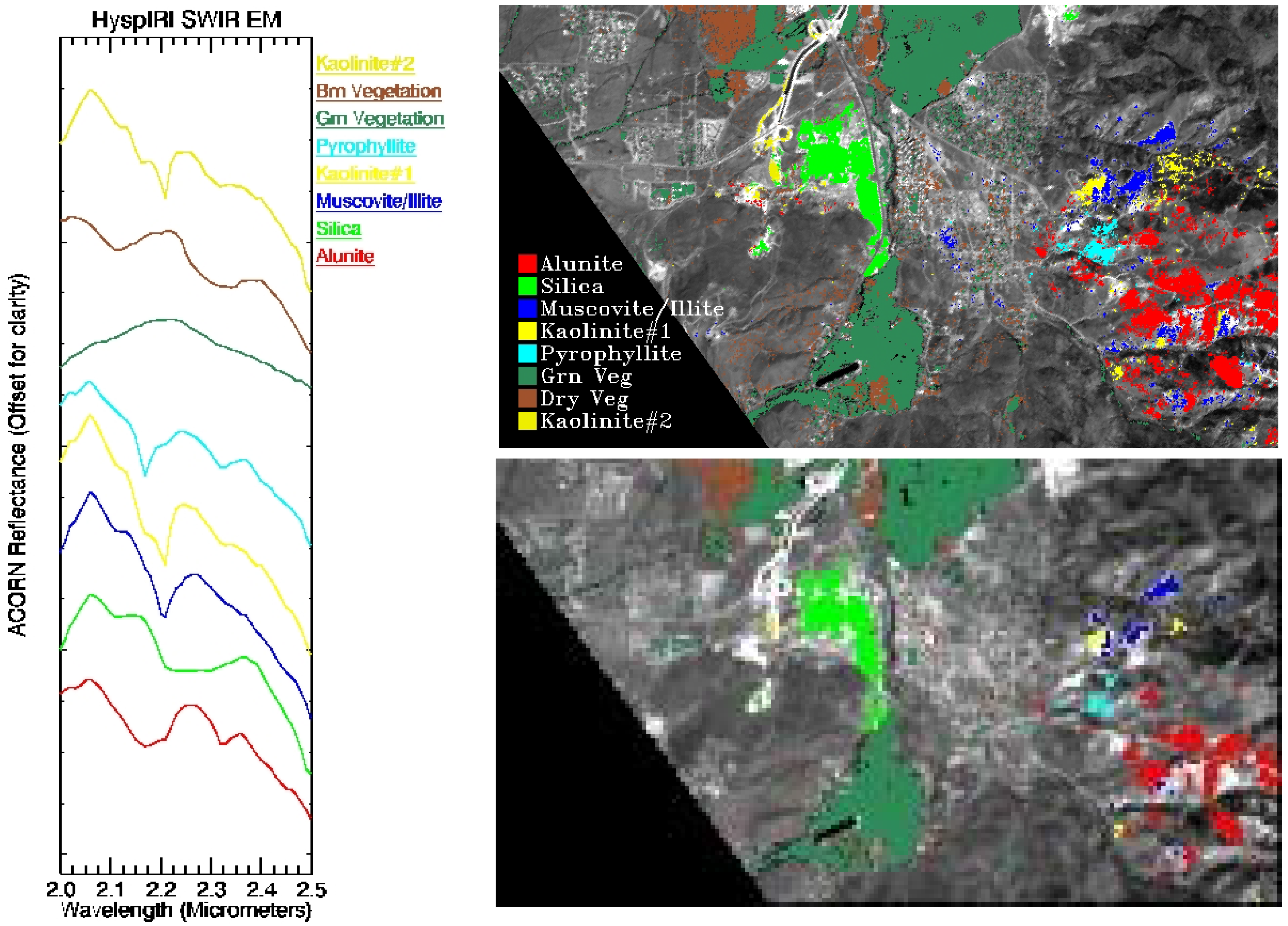
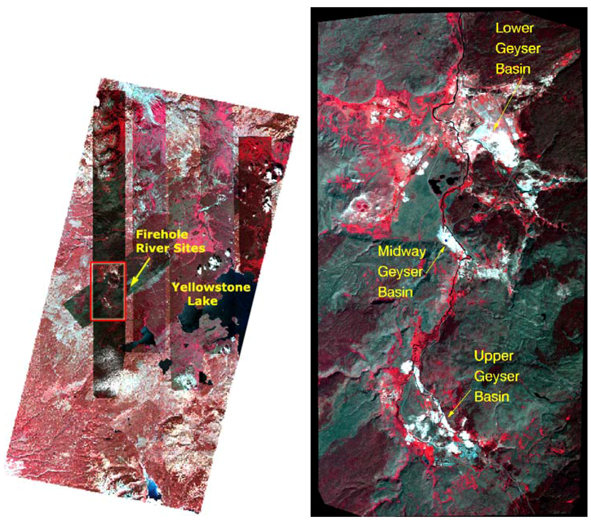
3.3. Yellowstone, WY Site (Active Geothermal System)

Yellowstone National Park covers nearly 3,500 square miles in the northwest corner of Wyoming and contains the largest concentration of geothermal features in the world [49]. The park has around 100 hot springs groups, totaling over 10,000 individual thermal features [50]. Yellowstone has been the site of extensive volcanism throughout the Cenozoic [51], with the geyser basins underlain entirely by Quaternary-age rhyolitic rocks [52]. Regional fault systems and the Yellowstone Caldera control the distribution of thermal features [53,54]. The entire area has been extensively glaciated, and many of the springs and geysers issue from stream and glacial sediments derived from the rhyolites [55].
Figure 5. Left: False color composite (color infrared or CIR) image of a portion of Yellowstone National Park. Yellowstone Lake can be used for location purposes. The large image base is two orthorectified ASTER images at 15 m spatial resolution. The ASTER image base is approximately 60 km. Also shown are 6 AVIRIS flightlines from 1997 orthorectified and overlain on the ASTER data for flightline location purposes. The Firehole River area 1996 AVIRIS subset described in the following sections (which fell along the same flightlines as the 1997 data) is outlined and labeled. Right: False color composite (color infrared or CIR) 1996 AVIRIS image of the Firehole River area. Each AVIRIS Image base in the left mosaic and the AVIRIS image base in the right image is approximately 10 km. North is to the top.
Remotesensing 03 01584 g005
Yellowstone contains numerous active examples of several types of hot springs–alkaline-type (Upper, Midway, and Lower Geyser Basins. referred to here as the “Firehole River area”), travertine (Mammoth Hot Springs), acidic types (Mud Volcano area) and mixed types (Norris Geyser Basin). AVIRIS data were acquired for portions of Yellowstone National park during 1996, 1997, and 1998 (Figure 5). Only selected results from 1996 data of the Firehole River area (Figure 6) are shown here. The Upper, Midway, and Lower Geyser Basins of Yellowstone National Park occur along the Firehole River in the west central part of the park (Figure 5). The Upper Basin, containing over 150 hot springs and geysers, extends approximately 5 km northwest from Old Faithful along both sides of the river [56]. The large majority of thermal features have high flow, alkaline-composition waters, many of which commonly discharge directly into the river. Some acid-dominated systems occur along the fringes of the basin, characterized by low flow and minimal deposition of sinter and sulfur. Midway Basin occurs downstream along the Firehole River and contains approximately 30 springs with predominantly alkaline chemistry, including the largest single hot spring in the world, the Grand Prismatic Spring, which is more than 100 m across. The Lower Geyser Basin is the largest of all of the Yellowstone geyser areas, characterized by large, deep hot springs and alkaline geysers covering an area of approximately 40 km2. As in the Upper Geyser Basin, surrounding slopes and ridges characteristically have acid springs, mud pots, and fumaroles; some of the acid features, however, occur in close proximity to alkaline hot springs [50].
The AVIRIS data of Yellowstone analyzed here for the Firehole River site were acquired 6 August 1996 at approximately 15 m spatial resolution. They were atmospherically corrected to reflectance, spectrally resampled to HyspIRI spectral resolution, geocorrected to orthorectified ASTER data, and spatially resampled to 60 m resolution as previously described. The standardized hyperspectral data analysis procedures were followed for the Firehole River area on simulated HyspIRI SWIR data only (2.0–2.5 μm) at both 15 m and 60 m spatial resolution.
Figure 6. Left: SWIR spectral endmembers for the 1996 Firehole River 15 m HyspIRI spectrally resampled AVIRIS data. Center: 15 m mixture-tuned-matched-filtering (MTMF) spectral mapping results for the spectral endmembers shown on the left. Right: 60 m MTMF spectral mapping results for 60 m HyspIRI-simulated data. Image base is approximately 10 km. North is to the top.
Remotesensing 03 01584 g006
The SWIR data were MNF transformed, the PPI was run to find potential endmembers, and n-Dimensional visualization was used to extract specific endmembers at 15 m spatial resolution (Figure 6, Left). Extracted 15 m mineral spectra were compared with the USGS spectral library for identification. The mineralogy determined was simple, principally hydrothermal silica and kaolinite. Both dry and green vegetation were also present. Several additional vegetation endmembers were also extracted (not shown). The 15 m SWIR endmembers were again used to perform mixture-tuned-matched-filtering (MTMF) mapping of the spectrally predominant mineral (or vegetation) for each pixel for the 15 m and 60 m HyspIRI-simulated data (Figure 6, Right).
The SWIR mineral mapping generally confirms the alkaline nature of the Firehole River area hot springs/geothermal system, as the principal mineral deposited is silica (sinter). There are also a few small areas of acid sulfate alteration, as evidenced by the occurrence of kaolinite in a few spots. The 60 m resolution simulated HyspIRI data mapped similar minerals and distributions to the 15 m data, with some loss of detail. These simulated data, while somewhat limited by low spatial resolution, appear adequate for mapping large geothermal systems such as Yellowstone. There are, however, other significant minerals at this site and at other sites in Yellowstone that have been previously mapped using approximately 2 to 6 m spatial resolution AVIRIS [14]. These unfortunately cannot be easily mapped using imaging spectrometry at the 15 and 60 m scales.
Accuracy assessment was also performed comparing the capability of the 60 m HyspIRI-simulated SWIR data to map the specific minerals identified at Yellowstone, Wyoming. The 60 m HyspIRI-simulated data were compared to the 15 m HyspIRI spectrally resampled data again using the confusion matrix approach [33]. The SWIR mineral mapping results shown above in Figure 6 were directly compared on a pixel-by-pixel basis using the 15 m mineral map as the “ground truth” (Table 3).
Table 3. Confusion matrix for Yellowstone, Wyoming, 15 m versus 60 m HyspIRI simulation. Overall Accuracy = (542160/775992) 69.8667%. Kappa Coefficient = 0.3441.
GroundTruth
ClassUnclassKaoliniteSilicaGrn VegDry VegTotal
Unclass76.8949.4112.8635.4451.6368.03
Kaolinite1.1219.150.360.451.031.11
Silica0.933.1869.172.341.412.84
Grn Veg5.625.618.7656.013.069.82
Dry Veg15.4422.658.855.7742.6618.20
Total100.00100.00100.00100.00100.00100.00
ClassCommissionOmissionProd. Acc.User Acc.
PercentPercentPercentPercent
Unclass15.9323.1176.8984.07
Kaolinite92.4980.8519.157.51
Silcia39.0930.8369.1760.91
Grn Veg49.3343.9956.0150.67
Dry Veg67.6557.3442.6632.35
Overall accuracy of the 60 m classification as compared to the 15 m classification for Yellowstone, Wyoming is estimated at approximately 70%. The calculated Kappa Coefficient, however, which assesses classification performance relative to chance, is only 0.34, falling into the generally accepted “Poor Agreement” category for the Kappa Coefficient statistic [34,35]. An examination of the diagonals of the confusion matrix shows accuracies ranging from approximately 19–69%. As seen for Steamboat Springs, Nevada, the best mapping results are for silica, which is nearly ubiquitous at the hot springs sites throughout Yellowstone in the form of large surface distributions of siliceous sinter. The worst mineral match is for the kaolinite class, which again occurs only as relatively small patches in the 15 m mineral map image. In the 60 m HyspIRI-simulated data the kaolinite exposures are small with respect to the 60 m pixel and thus were confused with other minerals and mostly dry vegetation (errors of commission), or not mapped at all (errors of omission) due to spectral mixing. The confusion matrix further shows that there is a fairly even split of errors of commission versus omission—both of which are high for most classes. The producer and user accuracies are both lower for the Yellowstone case than for the other two sites studied here. The kaolinite class in particular shows very poor classification accuracy. For the Yellowstone, Wyoming site, it appears from the classification images (Figure 6) and the confusion matrix (Table 3) that the HyspIRI sensor would perform adequately for mapping the hydrothermal silica alteration and vegetation at Yellowstone, however, there is significant loss of detail at the 60 m scale for kaolinite compared to the 15 m scale. Again, however, the overall mineralogy and patterns are preserved (particularly for hydrothermal silica), and the simulated HyspIRI data can be used to identify the main mineral (silica) and spatially map the geothermal system.

4. Conclusions

Five simulated HyspIRI datasets consisting were generated of VNIR-SWIR reflectance and LWIR temperature/emissivity at 60 m spatial resolution using existing NASA airborne data (AVIRIS and MASTER). Analysis of the SWIR data only for the Cuprite, Nevada simulated HyspIRI dataset indicates that the proposed HyspIRI SWIR spectral response is essentially the same as AVIRIS, which has repeatedly demonstrated superior mineral mapping capabilities. Thus, HyspIRI-resampled AVIRIS data preserve key spectral information. MTMF mineral maps produced for three of the simulated datasets (Cuprite, Nevada; Steamboat Springs, Nevada; and Yellowstone, Wyoming) using the SWIR (2.0–2.5 μm) region only at both 15 m and 60 m spatial resolution successfully detected and mapped a wide variety of characteristic minerals, including jarosite, alunite, kaolinite, dickite, muscovite-illite, montmorillonite, pyrophyllite, calcite, buddingtonite, and hydrothermal silica at several fossil and active hydrothermal systems. Confusion matrix analyses of the datasets shows overall classification accuracy ranging from 70 to 92% for the 60 m HyspIRI simulated data relative to 15 m airborne spectrally resampled data. Errors of commission and omission provide insight to the causes of misclassification, clearly pointing towards scale dependent spectral mixing as the cause of most errors. Similar minerals and smaller areas of alteration are not mapped well by the simulated 60 m HyspIRI data due to spectral mixing with adjacent pixels.
These results demonstrate that HyspIRI data, while somewhat limited by their relatively coarse (60 m) spatial resolution, should be useful for mapping geologic materials associated with geothermal systems and ore deposits (fossil hydrothermal systems). Mineral mixing at the proposed 60 m spatial resolution does, however, complicate quantitative determination of surface mineralogy and will probably limit detection of some occurrences and detail observed using the airborne data. In addition, these results indicate that HyspIRI data should be useful for many other geologic applications requiring spectral data for mineral mapping.

Availability of Simulated Data

These simulated HyspIRI data will soon be made available for download via FTP. For additional information contact the corresponding author at [email protected].

Acknowledgments

This research was partially sponsored by NASA under NASA Grant NNX10AF99G at the University of Nevada, Reno (UNR). Portions of this effort were also partially supported by the Arthur Brant Laboratory for Exploration Geophysics at UNR. Additional research and manuscript preparation was done after the corresponding author changed employment from UNR to the Naval Postgraduate School, Monterey, CA. Ormat Nevada Inc. provided access to their geothermal properties for reconnaissance, field verification, and field spectral measurements.

References

  1. Goetz, A.F.H.; Vane, G.; Solomon, J.E.; Rock, B.N. Imaging spectrometry for earth remote sensing. Science 1985, 228, 1147–1153. [Google Scholar] [CrossRef] [PubMed]
  2. Kruse, F.A.; Perry, S.L. Improving multispectral mapping by spectral modeling with hyperspectral signatures. J. Appl. Remote Sens. 2009, 3, 033504. [Google Scholar]
  3. Hamilton, M.K.; Davis, C.O.; Rhea, W.J.; Pilorz, S.H.; Carder, K.L. Estimating chlorophyll content and bathymetry of Lake Tahoe using AVIRIS data. Remote Sens. Environ. 1993, 44, 217–230. [Google Scholar] [CrossRef]
  4. Roberts, D.A.; Smith, M.O.; Adams, J.B. Green vegetation, nonphotosynthetic vegetation, and soils in AVIRIS data. Remote Sens. Environ. 1993, 44, 255–269. [Google Scholar] [CrossRef]
  5. Clark, R.N.; Swayze, G.A.; Rowan, L.C.; Livo, K.E.; Watson, K. Mapping Surficial Geology, Vegetation Communities, and Environmental Materials in our National Parks: The USGS Imaging Spectroscopy Integrated Geology, Ecosystems, and Environmental Mapping Project. In Proceedings of Summaries of the 6th Annual JPL Airborne Earth Science Workshop, Pasadena, CA, USA, 4–8 March 1996; Volume 1, pp. 55–56.
  6. Green, R.O.; Dozier, J. Retrieval of Surface Snow Grain Size and Melt Water from AVIRIS Spectra. In Proceedings of the 6th Annual JPL Airborne Earth Science Workshop, Pasadena, CA, USA, 4–8 March 1996; Volume 1, pp. 127–134.
  7. Asner, G.P.; Green, R.O. Imaging spectroscopy measures desertification in the Southwest U.S. and Argentina. Eos Trans. AGU 2001, 80, 601–605. [Google Scholar] [CrossRef]
  8. Ungar, S.; Pearlman, J.; Mendenhall, J.; Reuter, D. Overview of the EARTH Observing One (EO-1) mission. IEEE Trans. Geosci. Remote Sens. 2003, 41, 1149–1159. [Google Scholar] [CrossRef]
  9. Taranik, J.V.; Aslett, Z.L. Development of hyperspectral imaging for mineral exploration. Rev. Econ. Geol. 2009, 16, 83–95. [Google Scholar]
  10. Kruse, F.A. Use of Airborne Imaging Spectrometer data to map minerals associated with hydrothermally altered rocks in the northern Grapevine Mountains, Nevada and California. Remote Sens. Environ. 1988, 24, 31–51. [Google Scholar] [CrossRef]
  11. Kruse, F.A.; Boardman, J.W.; Huntington, J.F. Evaluation and validation of EO-1 Hyperion for mineral mapping. IEEE Trans. Geosci. Remote Sens. 2003, 41, 1388–1400. [Google Scholar] [CrossRef]
  12. Kruse, F.A.; Perry, S.L.; Caballero, A. District-level mineral survey using airborne hyperspectral data, Los Menucos, Argentina. Ann. Geophys. 2006, 19, 83–92. [Google Scholar]
  13. Kratt, C.; Calvin, W.; Coolbaugh, M. Geothermal exploration with Hymap hyperspectral data at Brady–Desert Peak, Nevada. Remote Sens. Environ. 2006, 104, 313–324. [Google Scholar] [CrossRef]
  14. Livo, K.E.; Kruse, F.A.; Clark, R.N.; Kokaly, R.F.; Shanks, W.C., III. Hydrothermally altered rock and Hot-Spring Deposits at Yellowstone National Park—Characterized using airborne visible- and infrared-spectroscopy data. In Integrated Geoscience Studies in the Greater Yellowstone Area—Volcanic, Tectonic, and Hydrothermal Processes in the Yellowstone Geoecosystem; US Geological Survey Professional Paper 1717; USGS: Reno, NV, USA, 2007; Chapter O; pp. 493–505. [Google Scholar]
  15. NRC. National Research Council Committee on Earth Science and Applications from Space, Earth science and Applications from Space, National Imperatives for the Next Decade and Beyond; The National Academies Press: Washington, DC, USA, 2007. [Google Scholar]
  16. Kruse, F.A.; Coolbaugh, M.F.; Taranik, J.V.; Calvin, W.M.; Littlefield, E.F.; Michaels, J.; Martini, B.A. Characterization of Hydrothermal Systems Using Simulated Hyperspectral Infrared Imager (HysPIRI) Data. In Proceedings 2011 IEEE AeroSpace Conference, Big Sky, MT, USA, 5–12 March 2011.
  17. Porter, W.M.; Enmark, H.E. System overview of the Airborne Visible/Infrared Imaging Spectrometer (AVIRIS). SPIE 1987, 834, 22–31. [Google Scholar]
  18. Green, R.O.; Cone, J.E.; Margolis, J.; Chovit, C.; Faust, J. In-Flight Calibration and Validation of the Airborne Visible/Infrared Imaging Spectrometer (AVIRIS). In Proceedings of the 6th Annual JPL Airborne Earth Science Workshop, Pasadena, CA, USA, 4–8 March 1996; Volume 1, pp. 115–126.
  19. Green, R.O.; Eastwood, M.L.; Sarture, C.M. Imaging Spectroscopy and the Airborne Visible Infrared Imaging Spectrometer (AVIRIS). Remote Sens. Environ. 1998, 65, 227–248. [Google Scholar] [CrossRef]
  20. Green, R.O. AVIRIS and related 21st century imaging spectrometers for earth and space science. In High Performance Computing in Remote Sensing; Chapman and Hall/CRC: Boca Raton, FL, USA, 2007; pp. 335–358. [Google Scholar]
  21. Yamaguchi, Y.; Kahle, A.B.; Tsu, H.; Kawakami, T.; Pniel, M. Overview of advanced spaceborne thermal emission reflectance radiometer. IEEE Trans. Geosci. Remote Sens. 1998, 36, 1062–1071. [Google Scholar] [CrossRef]
  22. IMSPEC LLC. ACORN 6 User’s Manual; IMSPEC LLC: Palmdale, CA, USA, 2010; p. 121. [Google Scholar]
  23. Kruse, F.A. Comparison of ATREM, ACORN, and FLAASH Atmospheric Corrections Using Low-Altitude AVIRIS Data of Boulder, Colorado. In Proceedings 13th JPL Airborne Geoscience Workshop, Jet Propulsion Laboratory, Pasadena, CA, USA, 31 March–2 April 2004. JPL Publication 05-3.
  24. Kruse, F.A. Mapping surface mineralogy using imaging spectrometry. Geomorphology 2011. [Google Scholar] [CrossRef]
  25. Green, A.A.; Berman, M.; Switzer, P.; Craig, M.D. A Transformation for ordering multispectral data in terms of image quality with implications for noise removal. IEEE Trans. Geosci. Remote Sens. 1988, 26, 65–74. [Google Scholar] [CrossRef]
  26. Boardman, J.W. Automated Spectral Unmixing of AVIRIS Data Using Convex Geometry Concepts. In Proceedings of Summaries 4th JPL Airborne Geoscience Workshop, Pasadena, CA, USA, 25–29 October 1993; Volume 1, pp. 11–14.
  27. Boardman, J.W.; Kruse, F.A. Automated Spectral Analysis: A Geological Example Using AVIRIS Data, Northern Grapevine Mountains, Nevada. In Proceedings of Tenth Thematic Conference, Geologic Remote Sensing, San Antonio, TX, USA, 9–12 May 1994. I-407-I-418.
  28. Boardman, J.W. Analysis, understanding and visualization of hyperspectral data as convex sets in n-space. Proc. SPIE 1995, 2480, 14–22. [Google Scholar]
  29. Boardman, J.W. Leveraging the High Dimensionality of AVIRIS Data for Improved Sub-Pixel Target Unmixing and Rejection of False Positives: Mixture Tuned Matched Filtering. In Proceedings of Summaries of the Seventh Annual JPL Airborne Geoscience Workshop, Pasadena, CA, USA, 12–16 January 1998; Volume 1, p. 55.
  30. Swayze, G.A. The Hydrothermal and Structural History of the Cuprite Mining District, Southwestern Nevada: An Integrated Geological and Geophysical Approach. Ph.D. Dissertation, University of Colorado Boulder, Boulder, CO, USA, 1997. [Google Scholar]
  31. Abrams, M.J.; Ashley, R.P.; Rowan, L.C.; Goetz, A.F.H.; Kahle, A.B. Mapping of hydrothermal alteration in the Cuprite mining district, Nevada, using aircraft scanner images for the spectral region 0.46–2.36 micrometers. Geology 1977, 5, 713–718. [Google Scholar] [CrossRef]
  32. Clark, R.N.; Swayze, G.A.; Wise, R.; Livo, E.; Hoefen, T.; Kokaly, R.; Sutley, S.J. USGS Digital Spectral Library splib06a; Digital Data Series 231; US Geological Survey, 2007. Available online: http://speclab.cr.usgs.gov/spectral.lib06 (accessed on 18 July 2011).
  33. Richards, J.A.; Jia, X. Remote Sensing Digital Image Analysis: An introduction, 4th ed.; Springer: Berlin, Germany, 2006. [Google Scholar]
  34. Monserud, R.A.; Leemans, R. Comparing global vegetation maps with the Kappa-Statistic. Ecol. Modell. 1992, 62, 275–293. [Google Scholar] [CrossRef]
  35. Landis, J.R.; Koch, G.G. The measurement of observer agreement for categorical data. Biometrics 1977, 33, 159–174. [Google Scholar] [CrossRef] [PubMed]
  36. White, D.E. Thermal springs and epithermal ore deposits. Econ. Geol. 1955, 50, 99–154. [Google Scholar]
  37. White, D.E. Some principles of geyser activity, mainly from Steamboat Springs, Nevada. Am. J. Sci. 1967, 265, 641–684. [Google Scholar] [CrossRef]
  38. Silberman, M.L.; White, D.E.; Keith, T.E.C.; Docktor, R.D. Duration of Hydrothermal Activity at Steamboat Springs, Nevada, From Ages of the Spatially Associated Volcanic Rock; US Geological Survey Professional Paper 458-D; US GPO: Washington, DC, USA, 1979.
  39. White, D.E.; Thompson, G.A.; Sanberg, C.S. Rocks, Structure, and Geologic History of Steamboat Springs Thermal Area, Washoe County, Nevada; US Geological Survey Professional Paper 458-B; US GPO: Washington, DC, USA, 1964.
  40. Sigvaldason, G.E.; White, D.E. Hydrothermal Alteration in Drill Holes GS-5 and GS-7, Steamboat Springs, Nevada; US Geological Survey Professional Paper 450-D; US GPO: Washington, DC, USA, 1962; pp. D113–D117.
  41. White, D.E.; Anderson, E.T.; Grubbs, D.K. Geothermal brine well/mile-deep drill hole may tap ore-bearing magmatic water and rocks undergoing metamorphism. Science 1963, 139, 919–922. [Google Scholar] [CrossRef] [PubMed]
  42. Schoen, R.; White, D.E. Hydrothermal Alteration of Basaltic Andesite and Other Rocks in Drill Hole GS-6, Steamboat Springs, Nevada; US Geological Survey Professional Paper 575-B; US GPO: Washington, DC, USA, 1967; pp. 110–119.
  43. Schoen, R.; White, D.E.; Hemley, J.J. Argillization by descending acid at Steamboat Springs, Nevada. Clays Clay Minerals 1974, 22, 1–22. [Google Scholar] [CrossRef]
  44. White, D.E. Active geothermal systems and hydrothermal ore deposits. Econ. Geol. 1981, 75, 392–423. [Google Scholar]
  45. White, D.E.; Heropoulos, C.; Fournier, R.O. Gold and Other Minor Elements Associated with the Hot Springs and Geysers of Yellowstone National Park, Wyoming, Supplemented with Data from Steamboat Springs, Nevada; U.S. Geological Survey Bulletin 2001; US GPO: Washington, DC, USA, 1992; p. 10.
  46. Kruse, F.A. Characterization of Active Hot-Springs Environments Using Multispectral and Hyperspectral Remote Sensing. In Proceedings of 12th Thematic Conference, Applied Geologic Remote Sensing, Ann Arbor, MI, USA, 17–19 November 1997. I-214-I-221.
  47. Kruse, F.A. Mapping Hot Spring Deposits with AVIRIS at Steamboat Springs, Nevada. In Proceedings of the 8th JPL Airborne Earth Science Workshop, Pasadena, CA, USA, 8–11 February 1999; Jet Propulsion Laboratory Publication 99-17. pp. 239–246.
  48. Coolbaugh, M.F.; Taranik, J.V.; Kruse, F.A. Mapping of surface geothermal anomalies at Steamboat Springs, NV. using NASA Thermal Infrared Multispectral Scanner (TIMS) and Advanced Visible and Infrared Imaging Spectrometer (AVIRIS) data. In Proceedings of 14th Thematic Conference, Applied Geologic Remote Sensing, Las Vegas, NV, USA, 6–8 November 2000; pp. 623–630.
  49. Rhinehart, J.S. Geysers and Geothermal Energy; Springer-Verlag.: New York, NY, USA, 1980. [Google Scholar]
  50. Bryan, T.S. The Geysers of Yellowstone; Colorado Associated University Press: Boulder, CO, USA, 1986. [Google Scholar]
  51. Ruppel, E.T. Geology of Pre-Tertiary Rocks in the Northern Part of Yellowstone National Park, Wyoming; US Geological Survey Professional Paper 729-A; US GPO: Washington, DC, USA, 1972.
  52. Breckenridge, R.M.; Hinckley, B.S. Thermal Springs of Wyoming; Geological Survey of Wyoming Bulletin 60; US GPO: Washington, DC, USA, 1978.
  53. White, D.E.; Hutchinson, R.A.; Keith, T.E.C. The Geology and Remarkable Thermal Activity of Norris Geyser Basin, Yellowstone National Park, Wyoming; US Geological Survey Professional Paper 1456; US GPO: Washington, DC, USA, 1988.
  54. Eaton, G.P.; Christiansen, R.L.; Lyer, H.M.; Pitt, A.M.; Mabey, D.R.; Blank, H.R.J.; Zietz, I.; Gettings, M.E. Magma beneath Yellowstone National Park. Science 1975, 188, 787–796. [Google Scholar] [CrossRef] [PubMed]
  55. Pierce, K.L. History and Dynamics of Glaciation in the Northern Yellowstone Park Area; US Geological Survey Professional Paper 729-F; US GPO: Washington, DC, USA, 1979.
  56. Sorey, M.L. Geothermal Development and Changes in Surficial Features: Examples from the Western United States. In Proceedings of World Geothermal Congress 2000, Tohoku, Japan, 28 May–10 June 2000; pp. 705–711.

