AMARTIS v2: 3D Radiative Transfer Code in the [0.4; 2.5 µm] Spectral Domain Dedicated to Urban Areas


Abstract
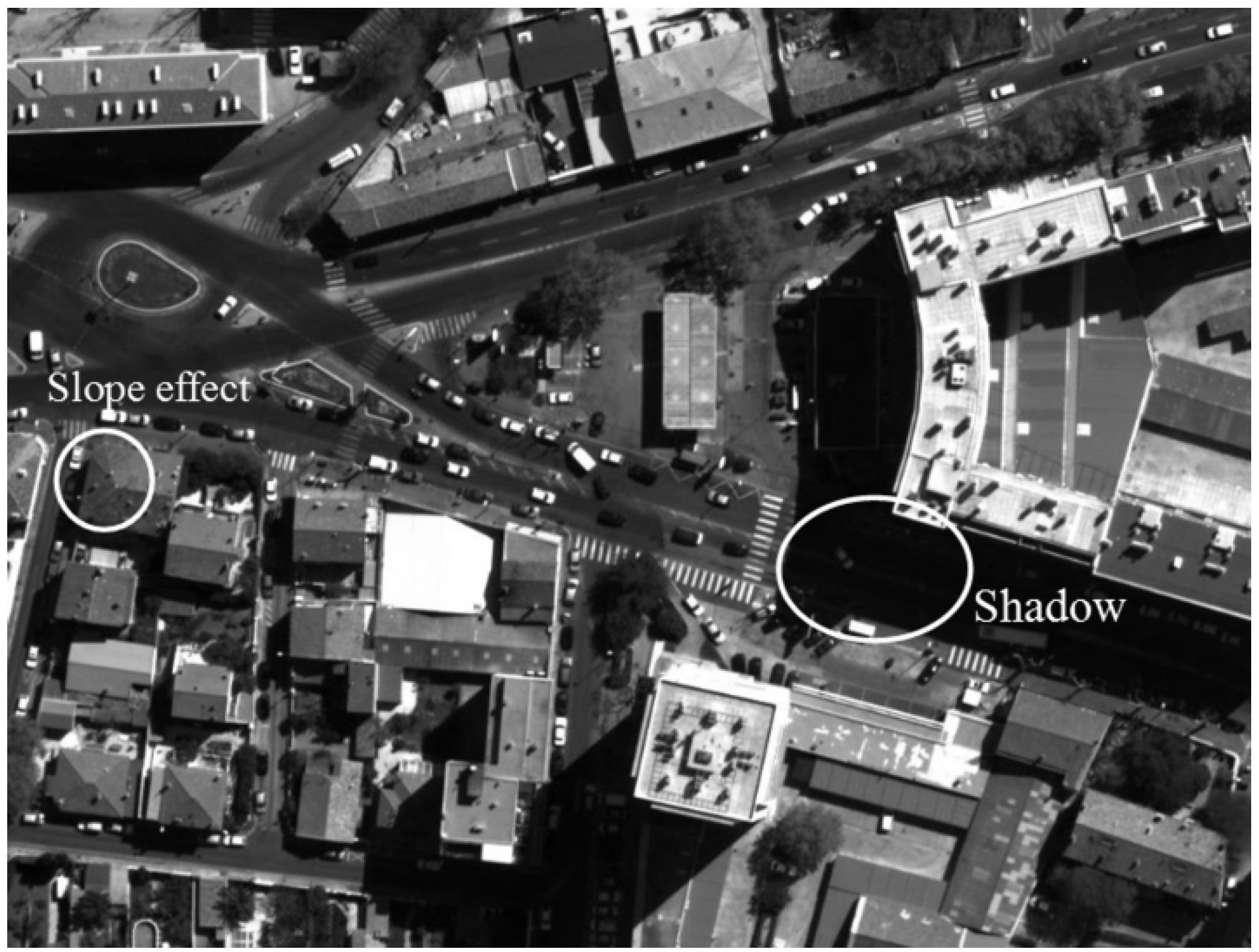
:1. Introduction

2. Description of the 3D Radiative Transfer Code AMARTIS v2
2.1. General Description
- The more realistic description of the atmosphere thanks to the coupling with 6S, especially the availability of new optical and geophysical aerosol models.
- The possibility of modeling realistic complex 3D scenes.
- The huge decrease of the computation time thanks to the use of an efficient ray-tracing tool for the Monte Carlo calculations.
2.2. Inputs Description
2.2.1. Scene

2.2.2. Atmosphere
2.2.3. Sensor
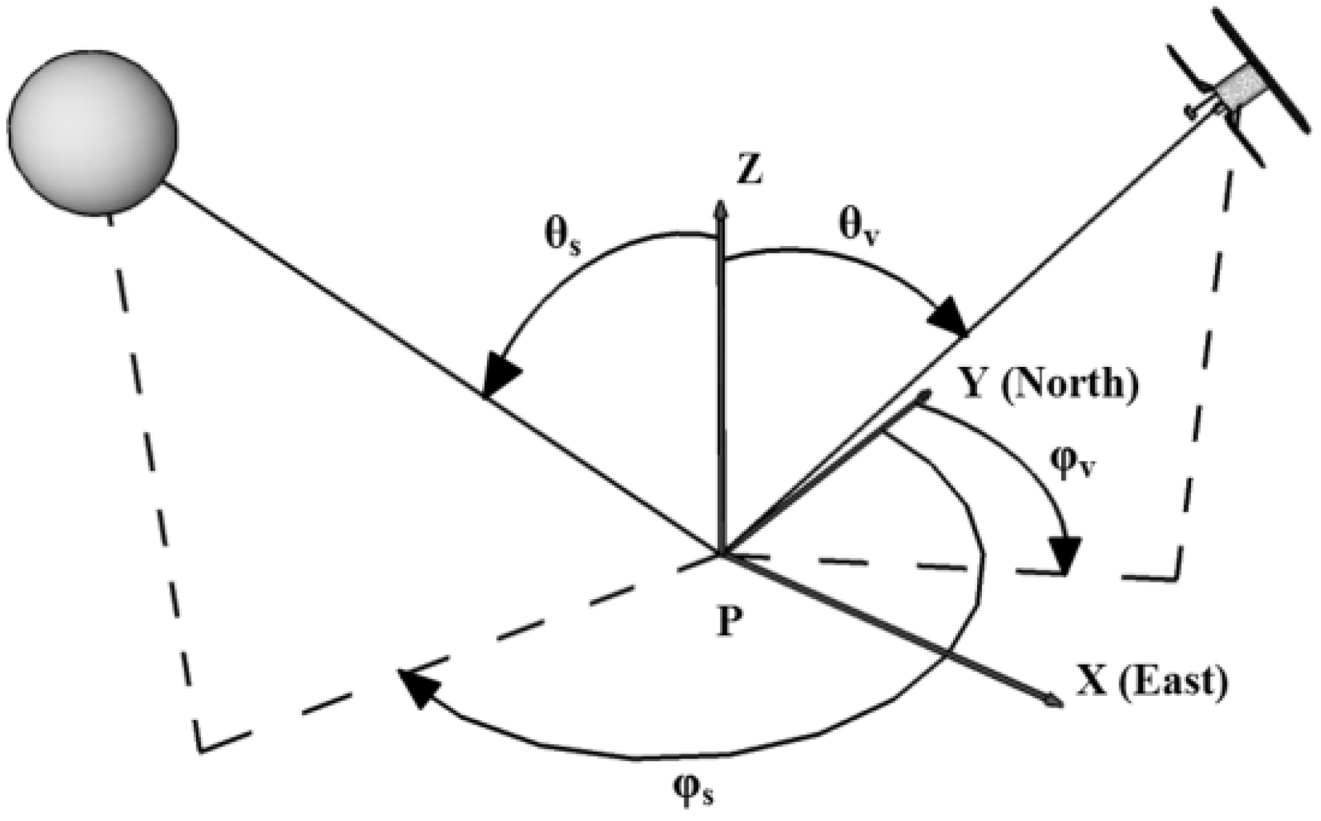
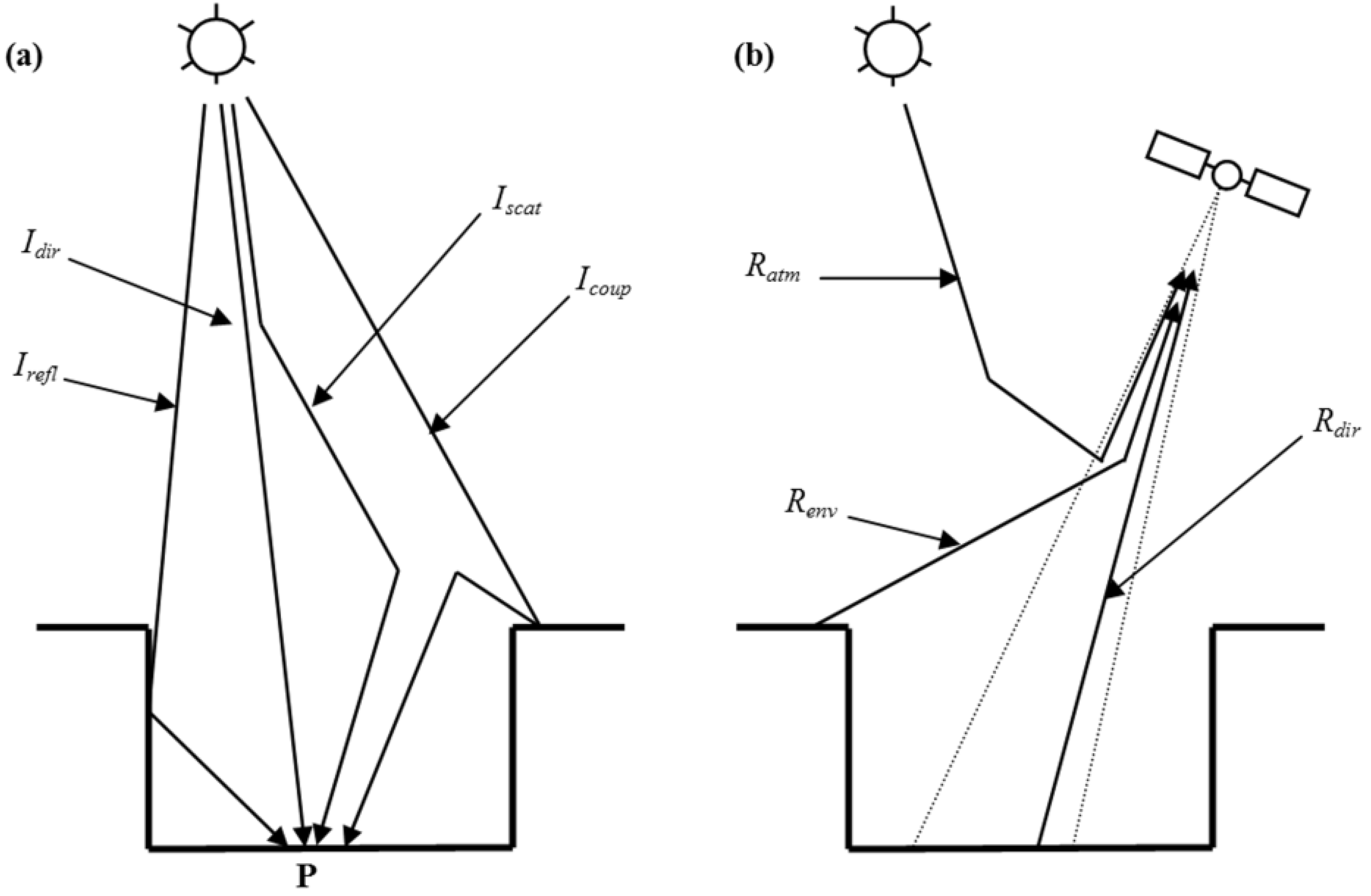
2.3. Method Description

3. Comparison of AMARTIS v2 with Existing Radiative Transfer Codes
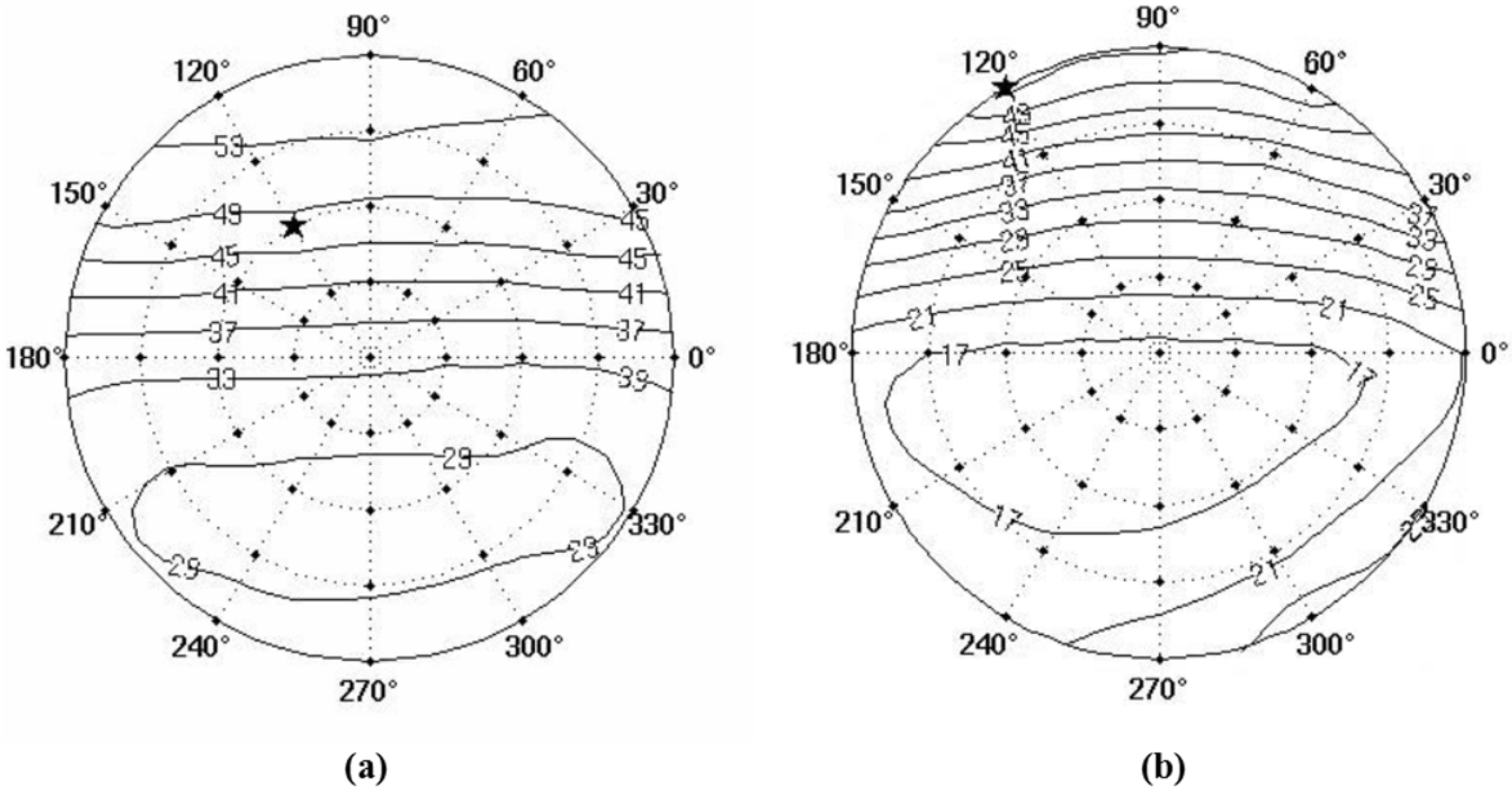
3.1. Comparison with AMARTIS v1


| Radiative component | σ | |
|---|---|---|
| Idir | 0.0% | 0.0% |
| Icoup | 8.9% | 5.3% |
| Irefl | 6.8% | 3.4% |
| Itot | 2.8% | 1.5% |
| Rdir | 2.9% | 1.4% |
| Renv | 3.0% | 1.5% |


3.2. Comparison with 6S
| Aerosols models | Single scattering albedo | Asymmetry factor |
|---|---|---|
| M1 | 0.6 | 0.6 |
| M2 | 0.6 | 0.9 |
| M3 | 0.9 | 0.6 |
| M4 | 0.9 | 0.9 |
| AMARTIS v2 values (W.m−2.µm−1) | Difference between AMARTIS v2 and 6S | ||||||
| Absolute difference (W.m−2.µm−1) | Difference normalized by Itot | ||||||
| Min | Mean | Max | Mean | Standard deviation | Mean | Standard deviation | |
| Idir | 171.80 | 474.06 | 1,132.67 | 0.23 | 0.33 | 0.03% | 0.03% |
| Iscat | 0.14 | 175.51 | 746.00 | 0.01 | 0.00 | 0.00% | 0.00% |
| Icoup | 0.06 | 17.40 | 60.43 | 3.34 | 4.06 | 0.42% | 0.37% |
| Itot | 188.85 | 666.98 | 1,348.58 | 3.46 | 4.23 | 0.43% | 0.39% |
| AMARTIS v2 values (W.m−2.µm−1) | Difference between AMARTIS v2 and 6S | ||||||
| Absolute difference (W.m−2.µm−1) | Difference normalized by Rtot | ||||||
| Min | Mean | Max | Mean | Standard deviation | Mean | Standard deviation | |
| Rdir | 10.11 | 27.38 | 67.26 | 0.12 | 0.12 | 0.21% | 0.16% |
| Ratm | 0.04 | 18.33 | 84.05 | 0.00 | 0.00 | 0.01% | 0.01% |
| Renv | 0.01 | 7.27 | 30.24 | 0.54 | 0.75 | 0.90% | 0.84% |
| Rtot | 11.26 | 52.97 | 121.53 | 0.43 | 0.67 | 0.74% | 0.71% |
4. Illustrations of the Improvements Brought by AMARTIS v2
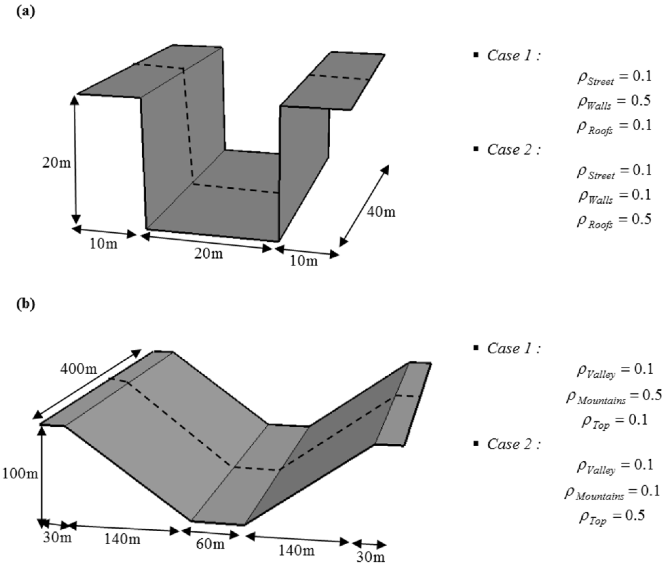
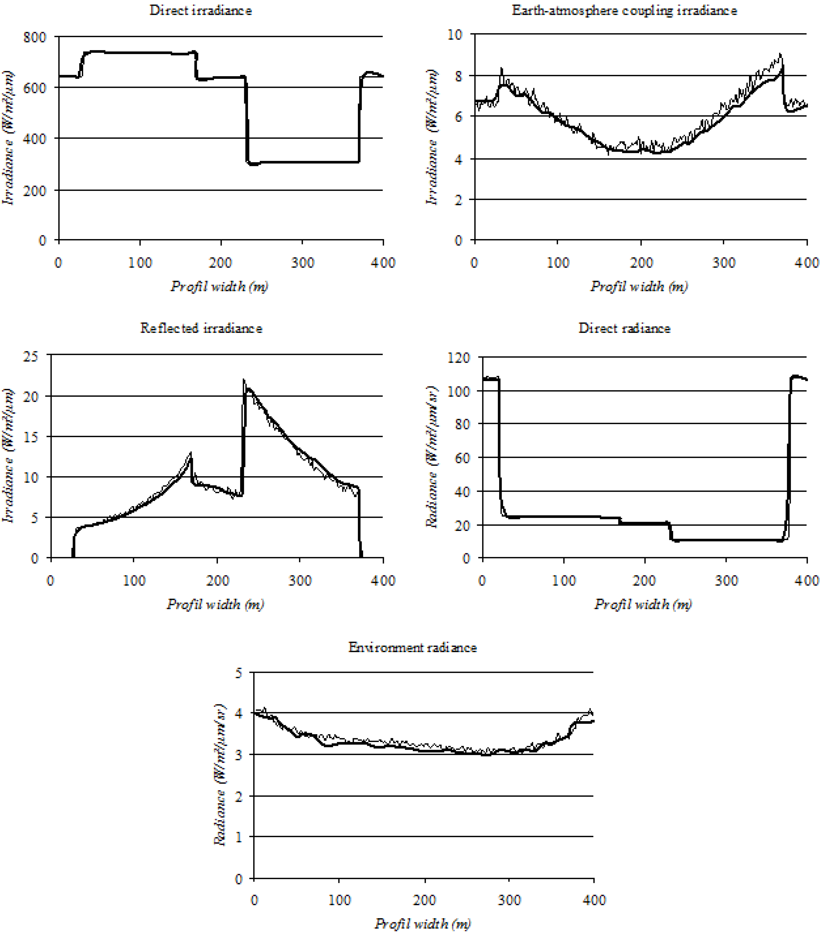
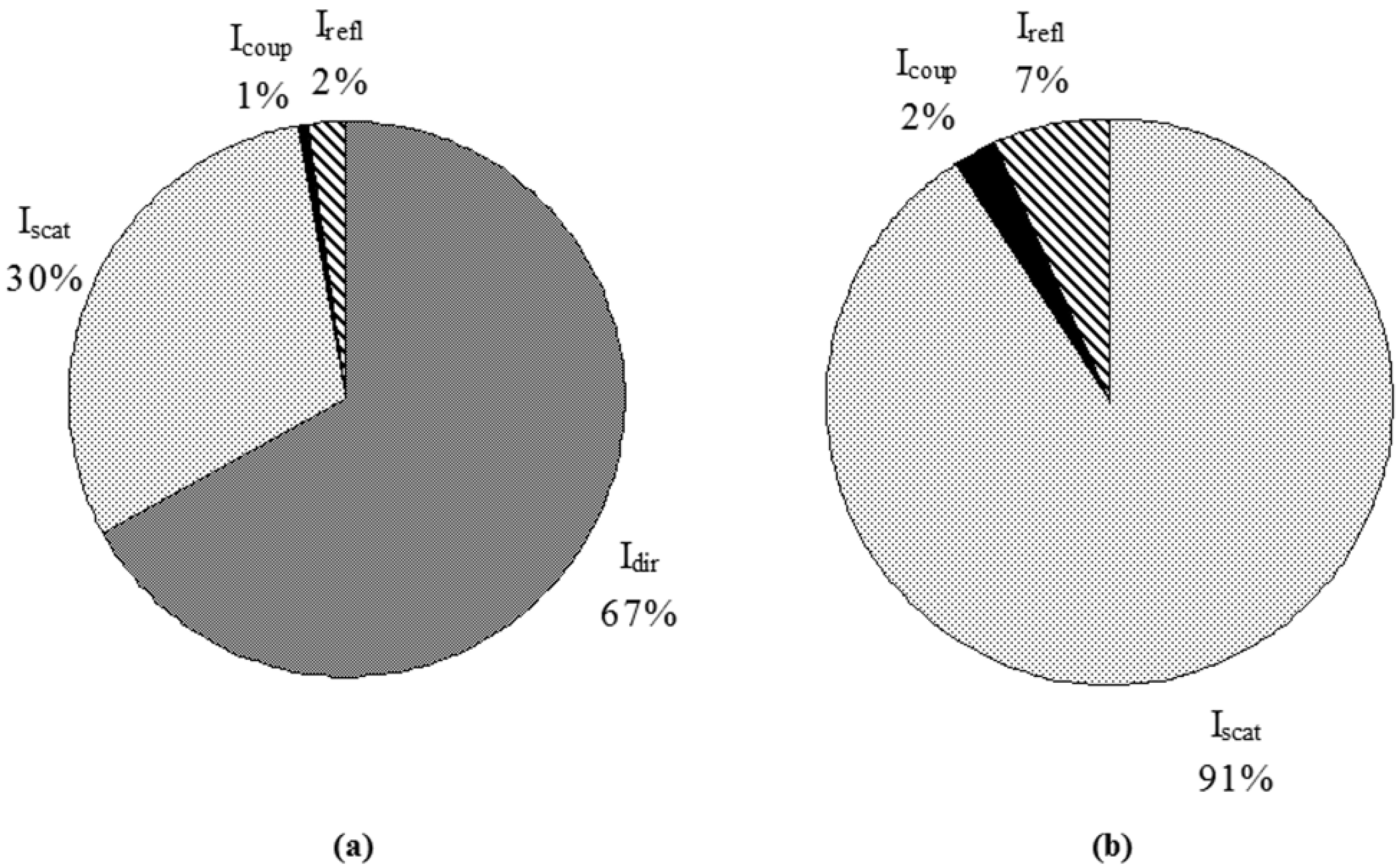
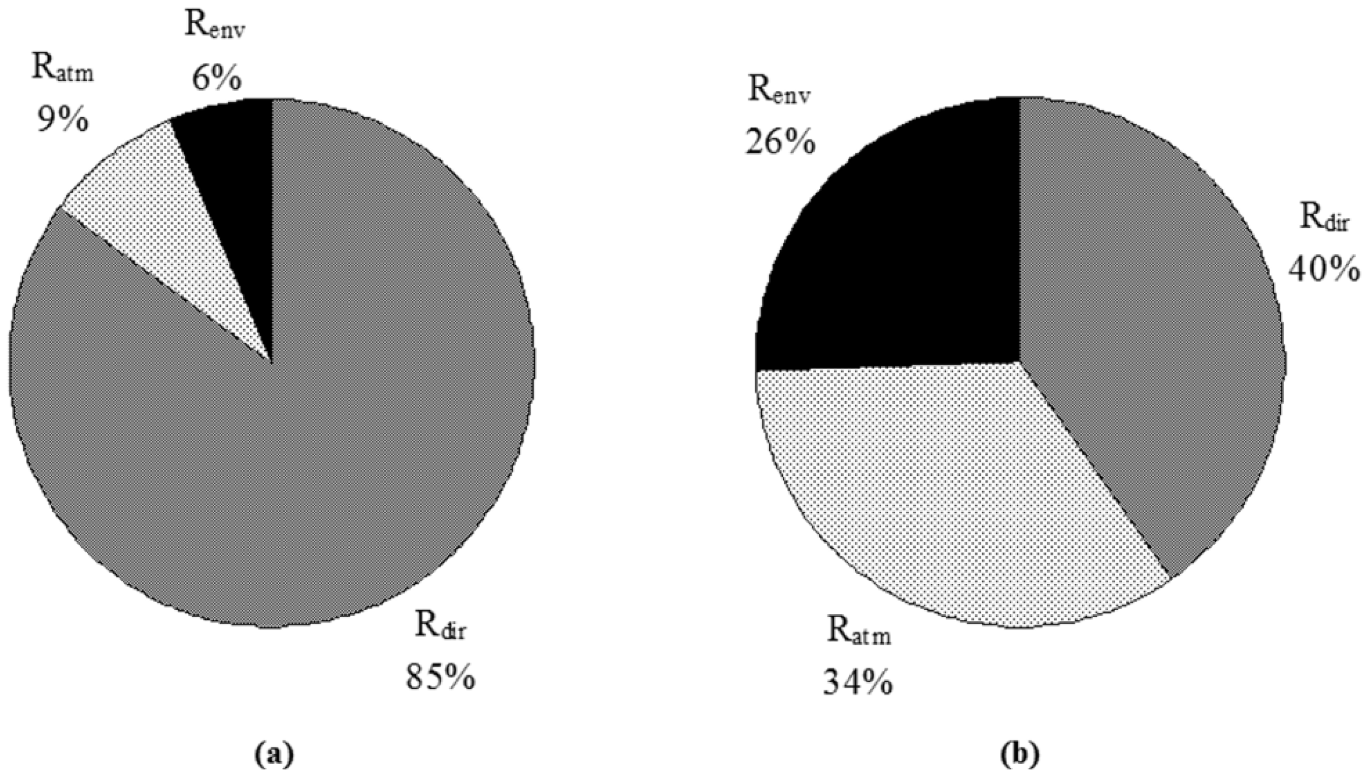
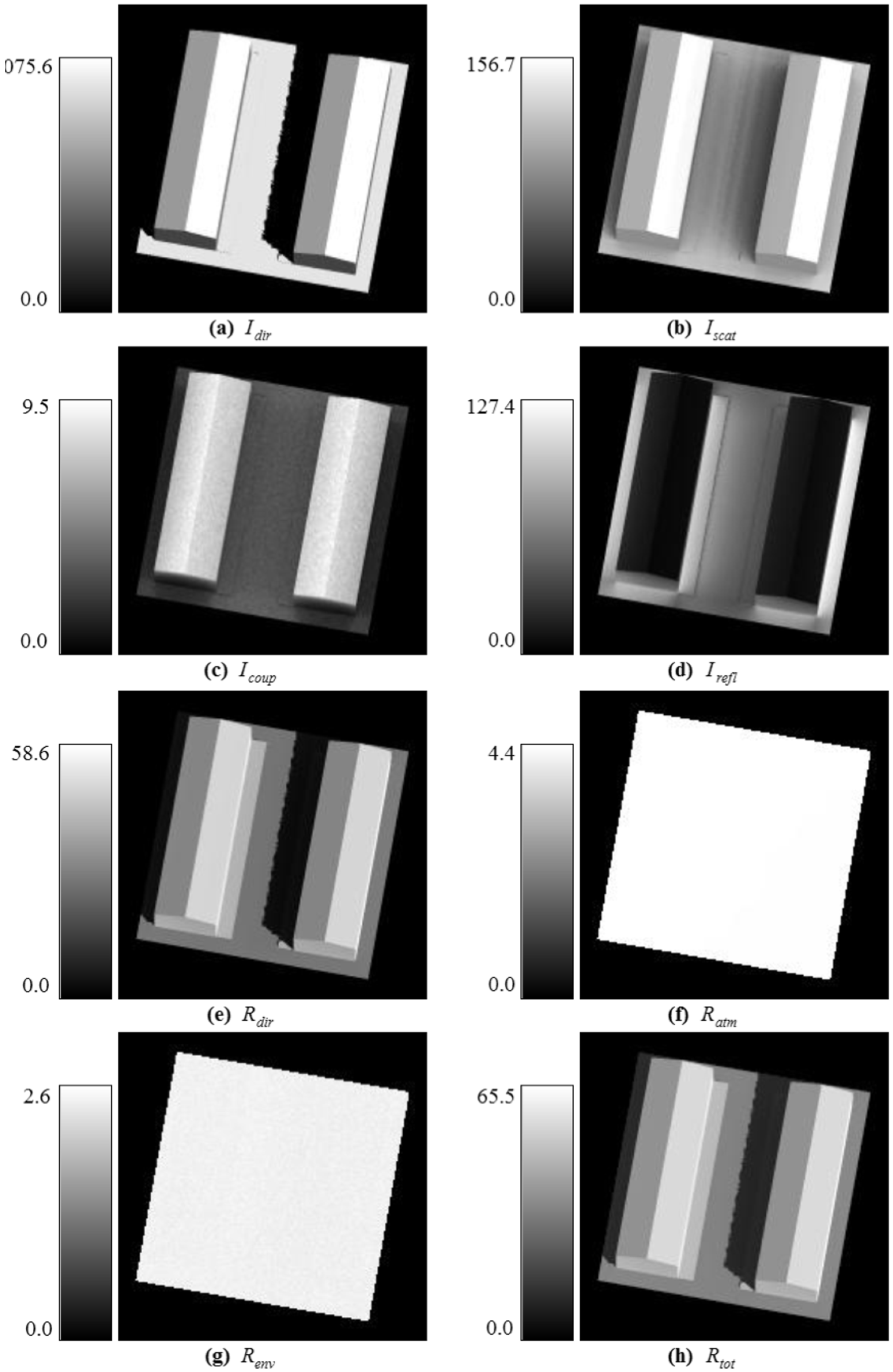
4.1. Case 1: Radiative Budget in an Urban Canyon
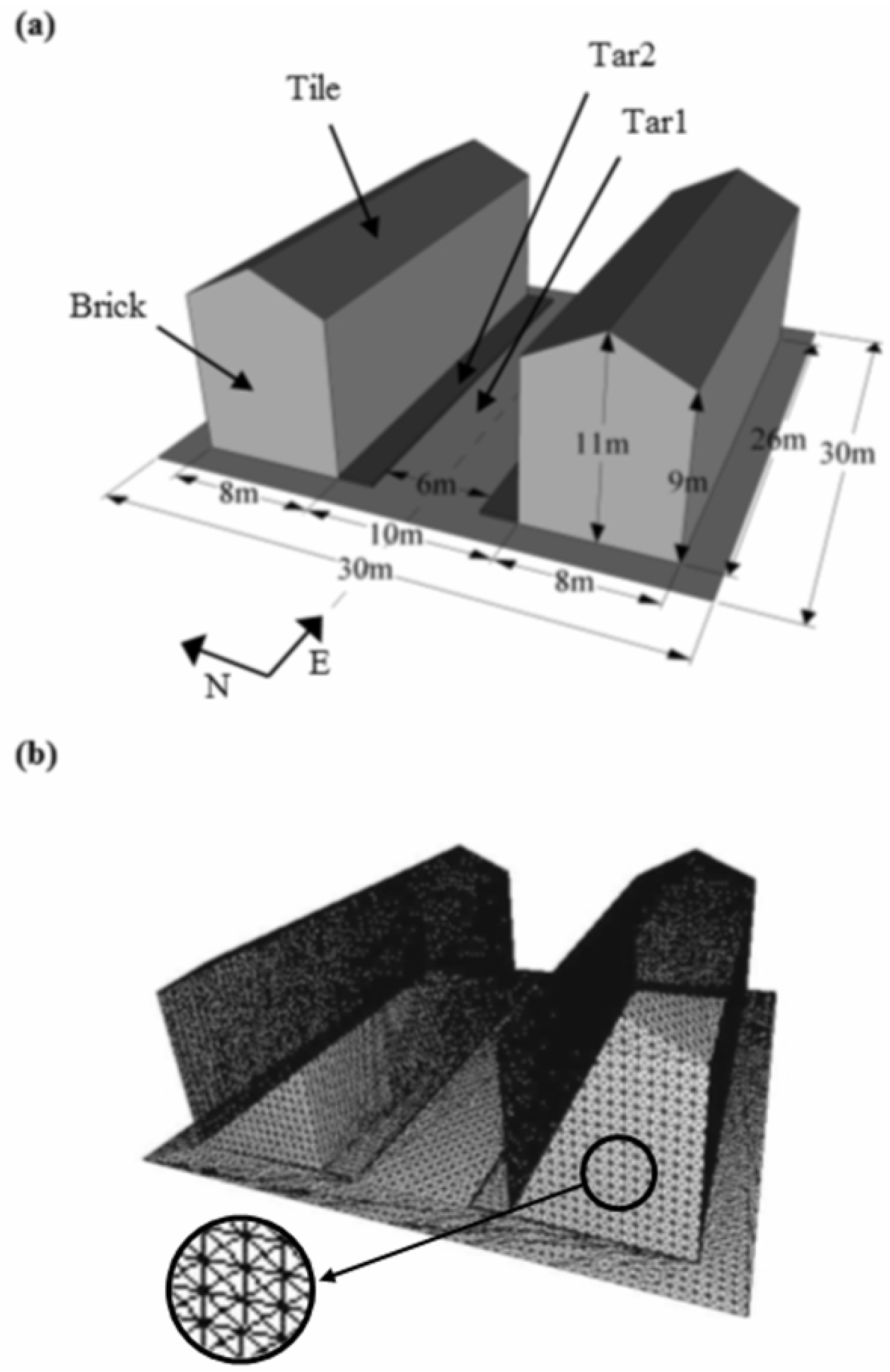
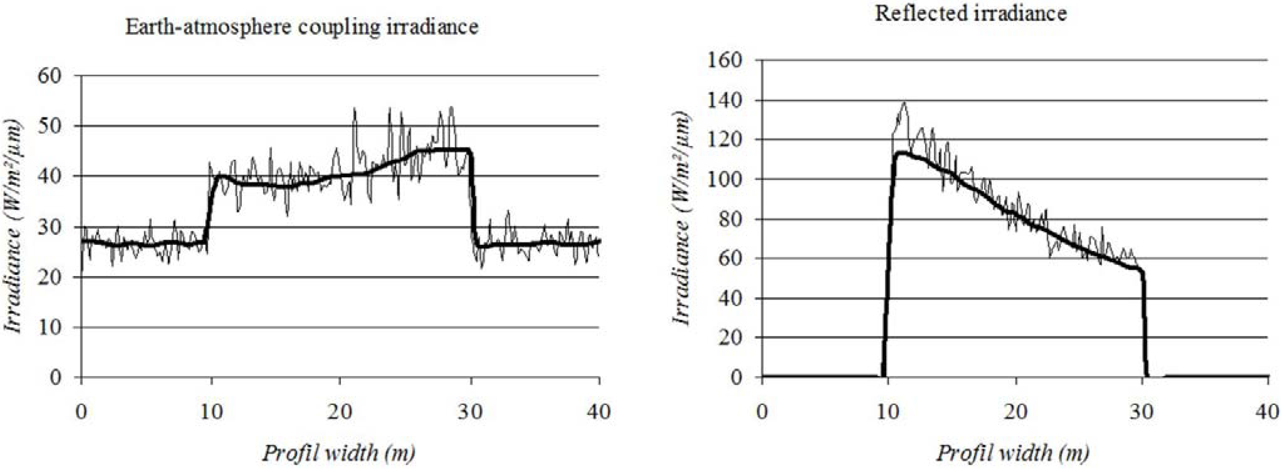
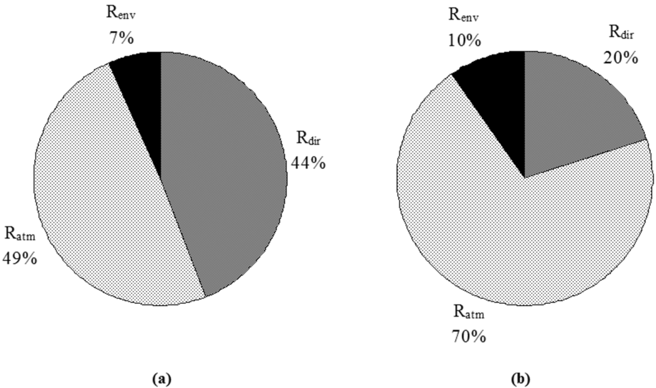
4.2. Case 2: Impact of Highly Reflective Windows

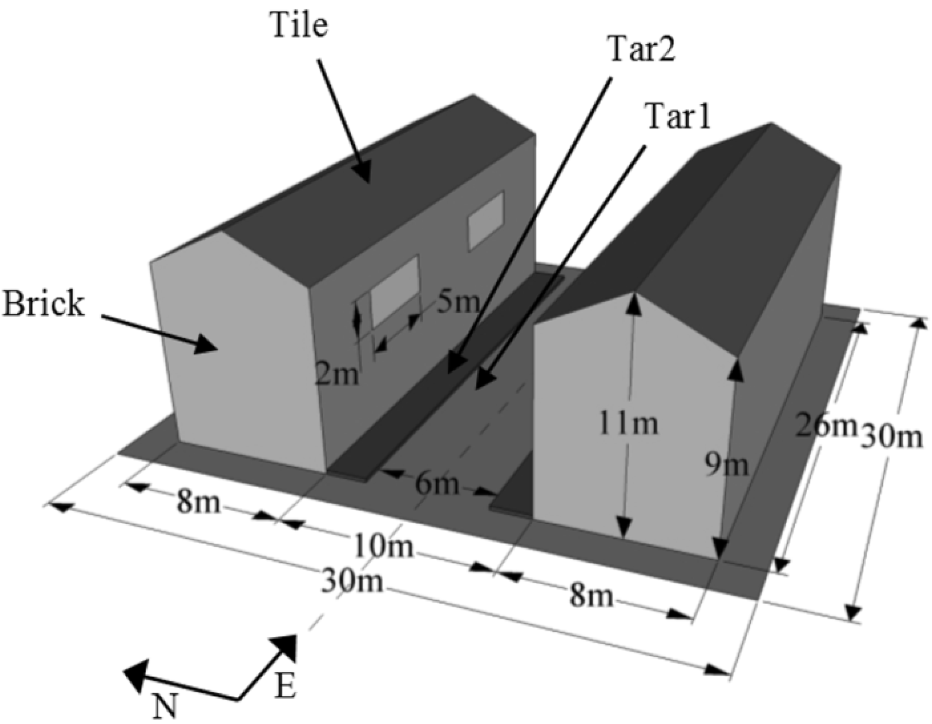

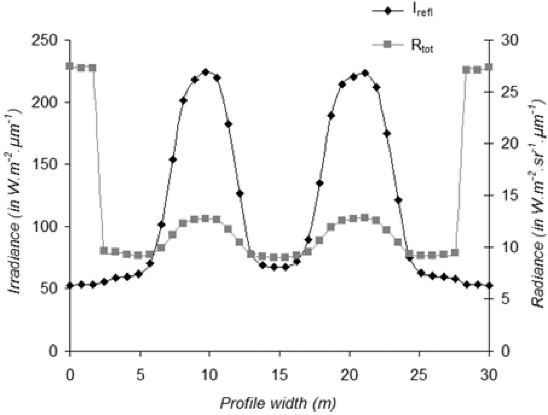
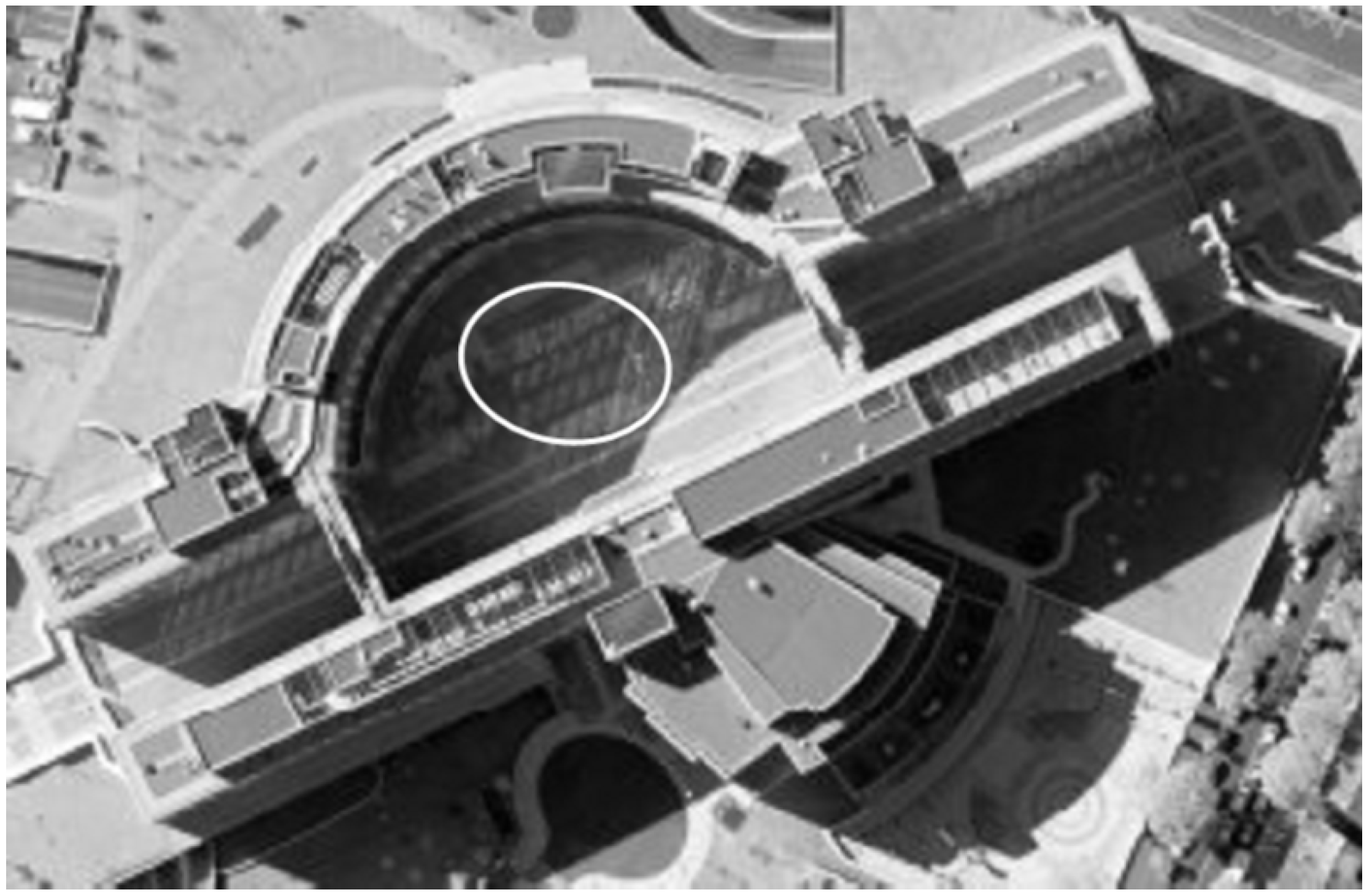
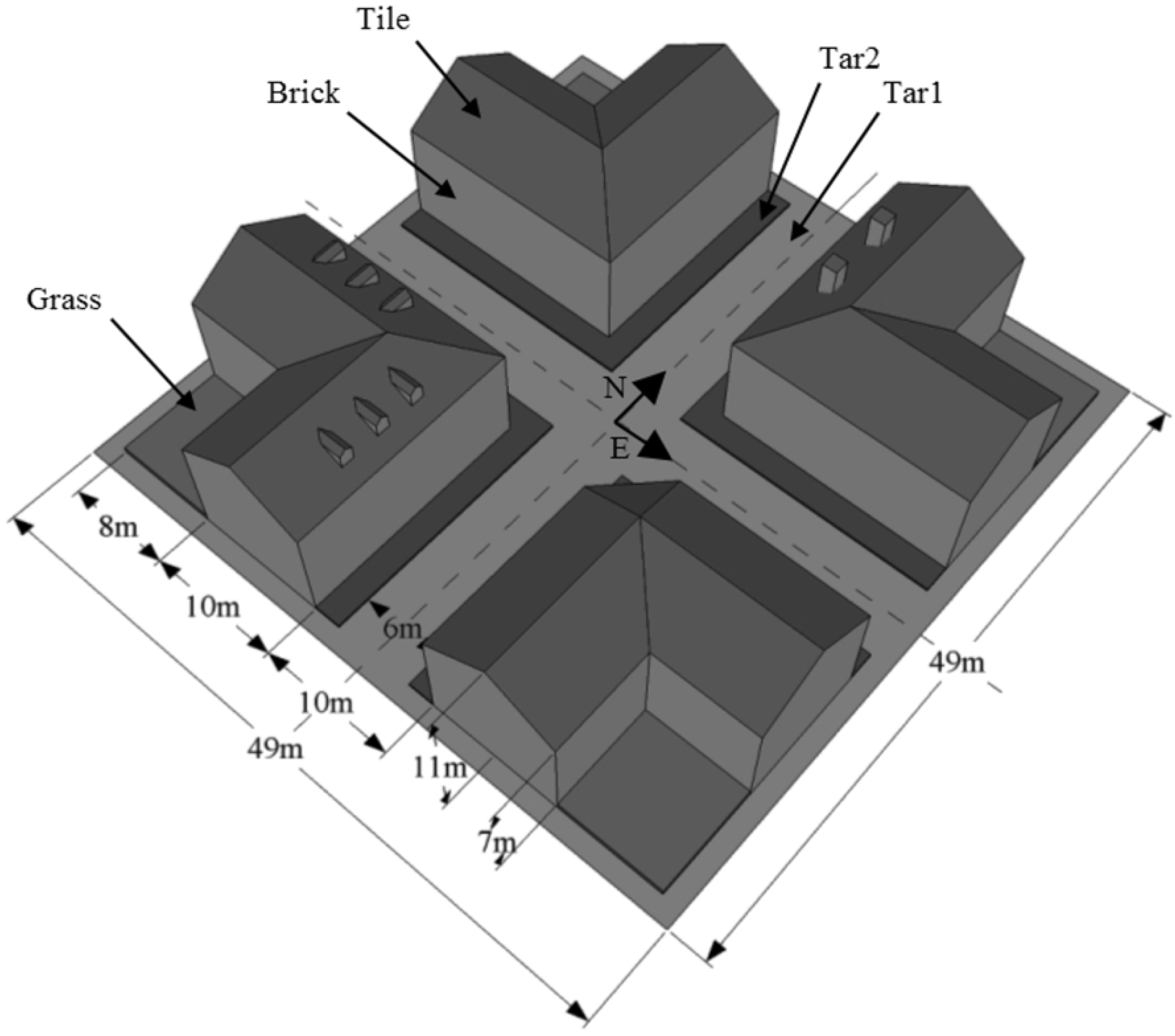
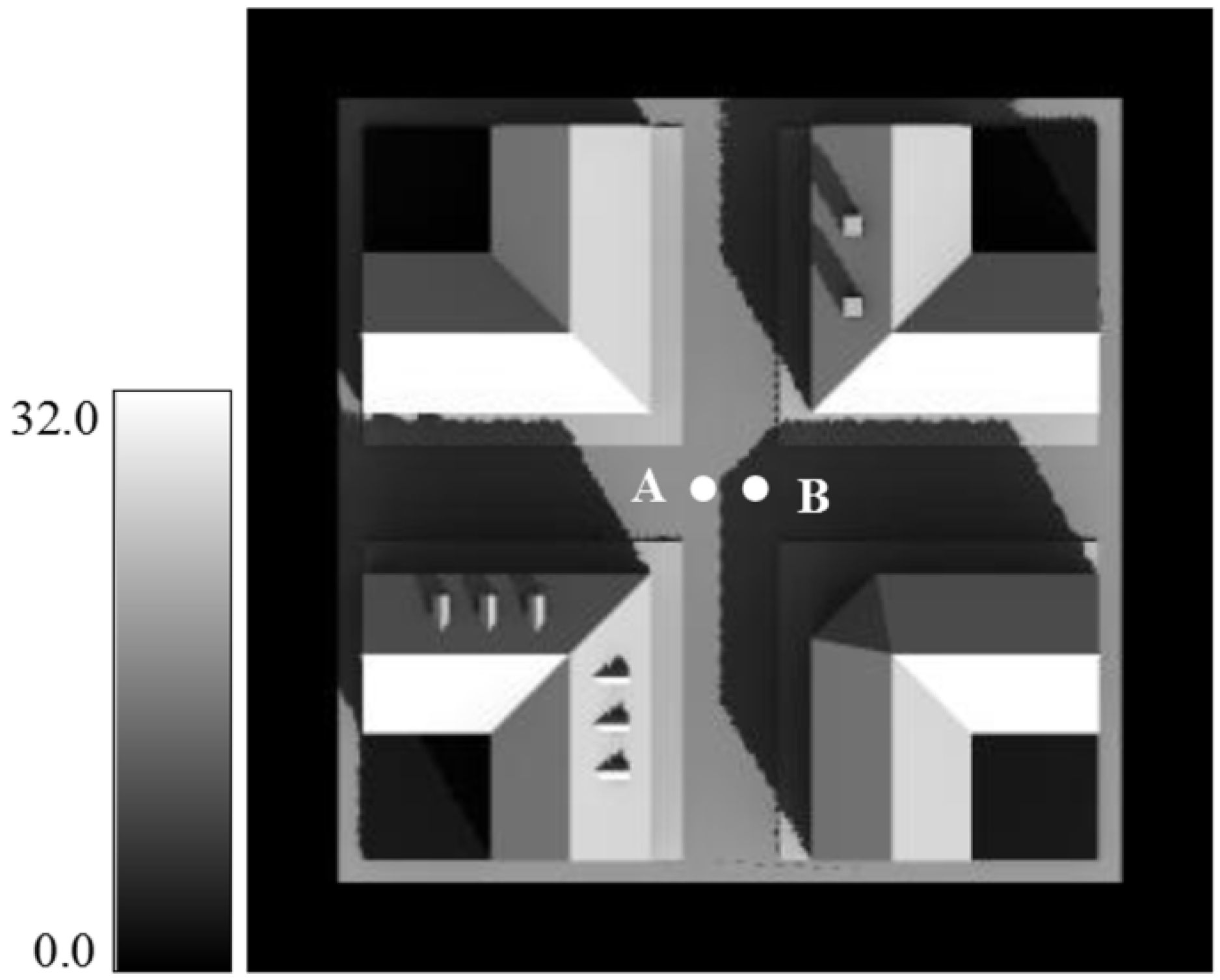
4.3. Case 3: Radiative Budget in a Crossroad in the Sun and in the Shade


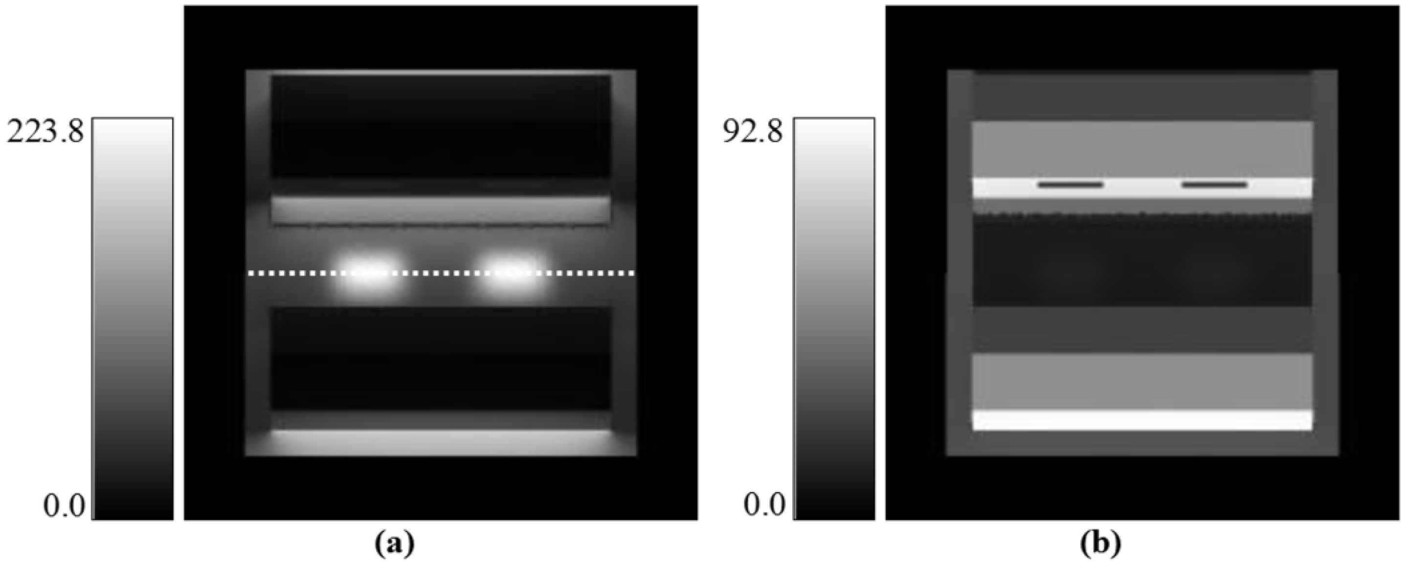
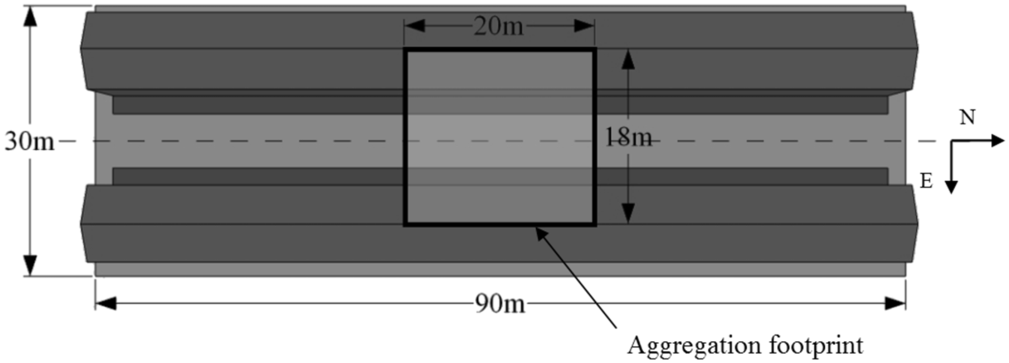
4.4. Case 4: Bidirectional Effects at the Street Scale


5. Conclusions and Perspectives
Acknowledgments
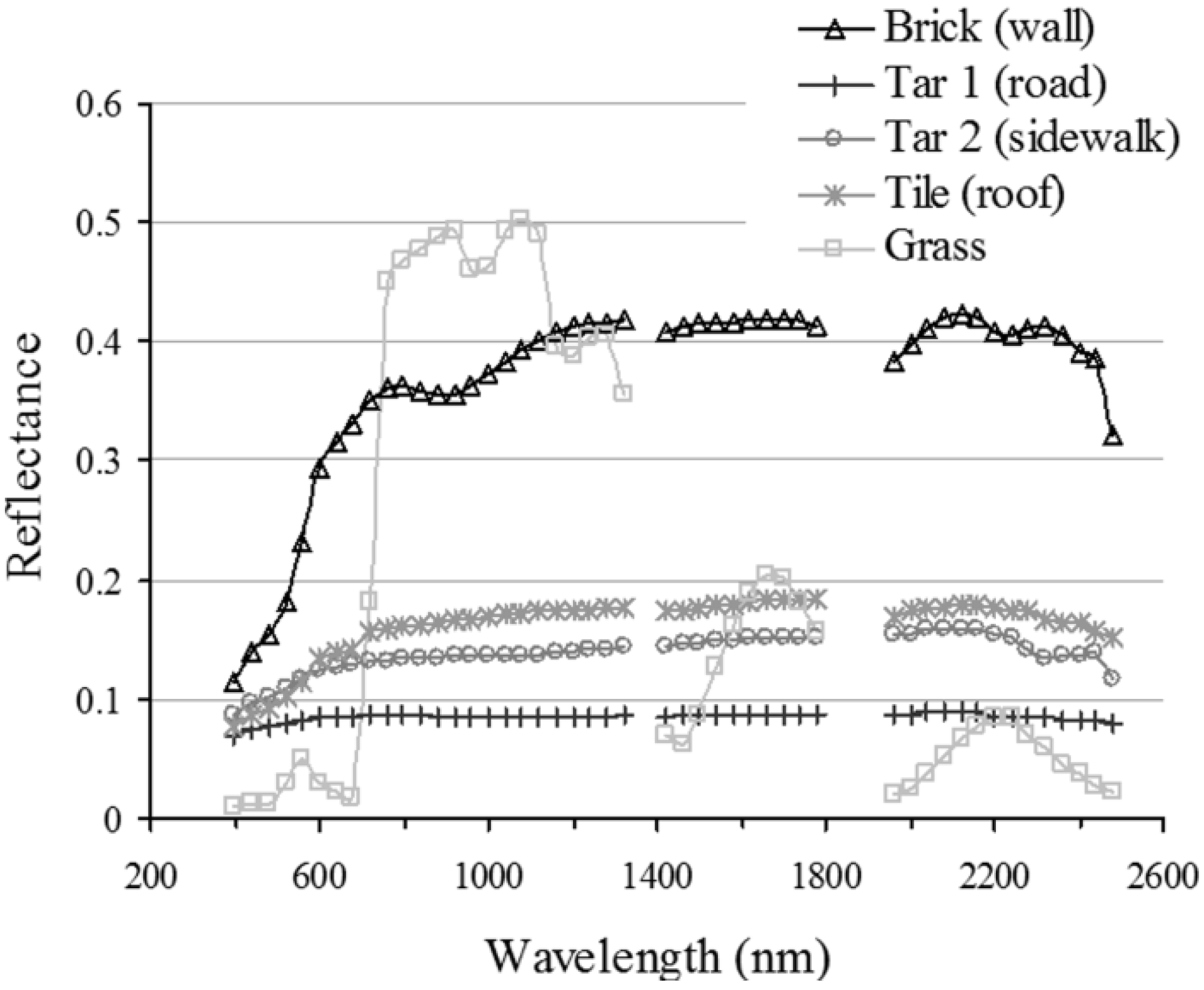
Appendix: Lambertian Reflectances Used in the AMARTIS v2 Computations
References
- Weng, Q.; Quattrochi, D.A. Urban Remote Sensing; CRC Press, Taylor and Francis: Oxford, UK, 2006. [Google Scholar]
- Xiao, J.; Shen, Y.; Ge, J.; Tateishi, R.; Tang, C.; Liang, Y.; Huang, Z. Evaluating urban expansion and land use change in Shijiazhuang, China, by using GIS and remote sensing. Landscape Urban Plan. 2006, 75, 69–80. [Google Scholar] [CrossRef]
- Miller, R.B.; Small, C. Cities from space: Potential applications of remote sensing in urban environmental research and policy. Eviron. Sci. Policy 2003, 6, 129–137. [Google Scholar] [CrossRef]
- Masson, V. Urban surface modeling and the meso-scale impact of cities. Theor. Appl. Climatol. 2006, 84, 35–45. [Google Scholar] [CrossRef]
- Lachérade, S.; Miesch, C.; Boldo, D.; Briottet, X.; Valorge, C.; Le Men, H. ICARE: A physically-based model to correct atmospheric and geometric effects from high spatial and spectral remote sensing images over 3D urban areas. Meteorol. Atmos. Phys. 2008, 102, 209–222. [Google Scholar] [CrossRef]
- Heiden, U.; Segl, K.; Roessner, S.; Kaufmann, H. Determination of robust spectral features for identification of urban surface materials in hyperspectral remote sensing data. Remote Sens. Environ. 2007, 111, 537–552. [Google Scholar] [CrossRef]
- Herold, M.; Gardner, M.E.; Noronha, V.; Roberts, D.A. Spectrometry and hyperspectral remote sensing of urban road infrastructure. Online J. Space Commun. 2003, 3, 1–29. [Google Scholar]
- Ben-Dor, E.; Levin, N.; Saaroni, H. A spectral based recognition of the urban environment using the visible and near-infrared spectral region (0.4–1.1 µm). A case study over Tel-Aviv, Israel. Int. J. Remote Sens. 2001, 22, 2193–2218. [Google Scholar] [CrossRef]
- Déliot, P.; Duffaut, J.; Lacan, A. Characterization and calibration of a high resolution multi-spectral airborne digital camera. Proc. SPIE 2006, 6031. [Google Scholar] [CrossRef]
- Krause, K.S. Relative radiometric characterization and performance of the QuickBird high-resolution commercial imaging satellite. Proc. SPIE 2004, 5542. [Google Scholar] [CrossRef]
- Dial, G.; Bowen, H.; Gerlach, F.; Grodecki, J.; Oleszczuk, R. IKONOS satellite, imagery, and products. Remote Sens. Environ. 2003, 88, 23–36. [Google Scholar] [CrossRef]
- de Lussy, F.; Kubik, P.; Greslou, D.; Pascal, V.; Gigord, P.; Cantou, J.P. PLEIADES-HR Image System Products and Quality PLEIADES-HR Image System Products and Geometric Accuracy. In Proceedings of the International Society for Photogrammetry and Remote Sensing Workshop, Hannover, Germany, 17–20 May 2005.
- Roessner, S.; Segl, K.; Heiden, U.; Kaufmann, H. Automated differentiation of urban surfaces based on airborne hyperspectral imagery. IEEE Trans. Geosci. Remote Sens. 2001, 39, 1525–1532. [Google Scholar] [CrossRef]
- Chanussot, J.; Benediktsson, J.A.; Fauvel, M. Classification of remote sensing images from urban areas using a fuzzy possibilistic model. IEEE Geosci. Remote Sens. Lett. 2006, 3, 40–44. [Google Scholar] [CrossRef]
- Herold, M.; Roberts, D.A.; Gardner, M.E.; Dennison, P.E. Spectrometry for urban area remote sensing—Development and analysis of a spectral library from 350 to 2,400 nm. Remote Sens. Environ. 2004, 91, 304–319. [Google Scholar] [CrossRef]
- Vincent, D.A.; Nielsen, K.E.; Durkee, P.A.; Reid, J.S. Aerosol Optical Depth Retrievals from High-Resolution Commercial Satellite Imagery over Areas of High Surface Reflectance. In Proceedings of AGU Fall Meeting, San Francisco, CA, USA, 5–9 December 2005.
- Thomas, C.; Doz, S.; Briottet, X.; Santer, R.; Boldo, D.; Mathieu, S. Remote Sensing of Aerosols in Urban Areas: Sun/Shadow Retrieval Procedure from Airborne very High Spatial Resolution Images: First Results. In Proceedings of the 6th EARSeL SIG IS Workshop, Tel-Aviv, Israel, 16–19 March 2009.
- Thomas, C.; Doz, S.; Briottet, X.; Santer, R.; Boldo, D.; Mathieu, S. Remote Sensing of Aerosols in Urban Areas: Sun/Shadow Retrieval Procedure from Airborne very High Spatial Resolution Images. In Proceedings of the 2009 Joint Urban Remote Sensing Event, Shanghai, China, 20–22 May 2009.
- Vermote, E.F.; Tanre, D.; Deuzé, J.L.; Herman, M.; Morcrette, J.J. Second simulation of the satellite signal in the solar spectrum, 6S: An overview. IEEE Trans. Geosci. Remote Sens. 1997, 35, 675–686. [Google Scholar] [CrossRef]
- Berk, A; Anderson, G.P.; Bernstein, L.S.; Acharya, P.K.; Dothe, H.; Matthew, M.W. MODTRAN4 radiative transfer modelling for atmospheric correction. Proc. SPIE 1999, 3756, 348–353. [Google Scholar]
- Miesch, C.; Poutier, L.; Achard, V.; Briottet, X.; Lenot, X.; Boucher, Y. Direct and inverse radiative transfer solutions for visible and near-infrared hyperspectral imagery. IEEE Trans. Geosci. Remote Sens. 2005, 43, 1552–1562. [Google Scholar] [CrossRef]
- Poutier, L.; Miesch, C.; Lenot, X.; Achard, V.; Boucher, Y. COMANCHE and COCHISE: Two Reciprocal Atmospheric Codes for Hyperspectral Remote Sensing. In Proceedings of the 2002 AVIRIS Earth Science and Applications Workshop, Pasadena, CA, USA, 5–8 March 2002.
- Gastellu-Etchegorry, J.P.; Martin, E.; Gascon, F. DART: A 3D model for simulating satellite images and studying surface radiation budget. Int. J. Remote Sens. 2004, 25, 73–96. [Google Scholar] [CrossRef]
- Miesch, C.; Briottet, X.; Kerr, Y.H. Phenomenological analysis of simulated signals observed over shaded areas in an urban scene. IEEE Trans. Geosci. Remote Sens. 2004, 42, 434–442. [Google Scholar] [CrossRef]
- Miesch, C.; Briottet, X.; Kerr, Y.H.; Cabot, F. Monte Carlo approach for solving the radiative transfer equation over mountainous and heterogeneous areas. Appl. Opt. 1999, 38, 7419–7430. [Google Scholar] [CrossRef] [PubMed]
- Miesch, C.; Briottet, X. Bidirectional reflectance of a rough anisotropic surface. Int. J. Remote Sens. Lett. 2002, 23, 3107–4114. [Google Scholar] [CrossRef]
- Junge, C.E. Air chemistry and Radiochemistry; Academic Press: New York, NY, USA, 1963. [Google Scholar]
- Thomas, C.; Briottet, X.; Santer, R.; Lachérade, S. Aerosols in urban areas: Optical properties and impact on the signal incident to an airborne high-spatial resolution camera. Proc. SPIE 2008, 7107. [Google Scholar] [CrossRef]
- Doz, S.; Thomas, C.; Lachérade, S.; Briottet, X.; Boldo, D.; Lier, P. Simulation of High Spatial Resolution Images for Urban Remote Sensing. In Proceedings of International Conference on Space Optics, Toulouse, France, 14–17 October 2008.
- Phong, B.T. Illumination for computer generated pictures. Commun. ACM 1975, 18, 311–317. [Google Scholar] [CrossRef]
- Cook, R.; Torrance, K. A reflectance model for computer graphics. ACM Trans. Graph. 1982, 1, 7–24. [Google Scholar] [CrossRef]
- Snyder, W.C.; Wan, Z. BRDF models to predict spectral reflectance and emissivity in the thermal infrared. IEEE Trans. Geosci. Remote Sens. 1998, 36, 214–225. [Google Scholar] [CrossRef]
- Miesch, C.; Briottet, X.; Kerr, Y.H.; Cabot, F. Radiative transfer solution for rugged and heterogeneous scene observations. Appl. Opt. 2000, 39, 6830–6846. [Google Scholar] [CrossRef] [PubMed]
- Herman, B.M.; Browning, S.R. A Numerical Solution to the equation of radiative transfer. J. Atmos. Sci. 1965, 22, 559–566. [Google Scholar] [CrossRef]
- Henyey, L.C.; Greenstein, J.L. Diffuse radiation in the galaxy. Astrophs. J. 1941, 93, 70–83. [Google Scholar] [CrossRef]
- Doz, S.; Thomas, C.; Briottet, X.; Lachérade, S. Simulation of at Sensor Signals over Urban Area: Two Cases Study. In Proceedings of the 2009 Joint Urban Remote Sensing Event, Shanghai, China, 20–22 May 2009.
- Rubin, M.; Powles, R.; von Rottkay, K. Models for the angle-dependent optical properties of coated glazing materials. Solar Energy 1999, 66, 267–276. [Google Scholar] [CrossRef]
- Dare, P.M. Shadow analysis in high-resolution satellite imagery of urban areas. Photogramm. Eng. Remote Sens. 2005, 71, 169–177. [Google Scholar] [CrossRef]
- Lachérade, S.; Miesch, C.; Briottet, X.; Le Men, H. Spectral variability and bidirectional reflectance behaviour of urban materials at a 20 cm spatial resolution in the visible and near infrared wavelengths—A case study over Toulouse (France). Int. J. Remote Sens. 2005, 26, 3859–3866. [Google Scholar] [CrossRef]
- Heiden, U.; Roessner, S.; Segl, K.; Kaufmann, H. Analysis of Spectral Signatures of Urban Surfaces for Their Area-Wide Identification Using Hyperspectral HyMap Data. In Proceedings of IEEE-ISPRS Joint Workshop on Remote Sensing and Data Fusion over Urban Areas, Rome, Italy, 8–9 November 2001; pp. 173–177.
- Ridd, M.K. Exploring a VIS (vegetation-impervious-surface-soil) model for urban ecosystem analysis through remote sensing: Comparative anatomy for cities. Int. J. Remote Sens. 1995, 16, 2165–2185. [Google Scholar] [CrossRef]
- Boardman, J.W.; Kruse, F.A.; Green, R.O. Mapping target signatures via partial unmixing of AVIRIS Data. In Summaries of the Fifth JPL Airborne Earth Science Workshop; JPL Publication 95-1; NASA: Pasadena, CA, USA, 23–26 January 1995; Volume 1, pp. 23–26. [Google Scholar]
- Segl, K.; Roessner, S.; Heiden, U.; Kaufmann, H. Fusion of spectral and shape features for identification of urban surface cover types using reflective and thermal hyperspectral data. ISPRS J. Photogramm. Remote Sens. 2003, 58, 99–112. [Google Scholar] [CrossRef]
- Jia, S.; Qian, Y. Spectral and spatial complexity-based hyperspectral unmixing. IEEE Trans. Geosci. Remote Sens. 2007, 45, 3867–3879. [Google Scholar]
- Rahman, M.T.; Alam, M.S. Nonlinear unmixing of hyperspectral data using BRDF and maximum likelihood algorithm. Proc. SPIE 2007, 6566. [Google Scholar] [CrossRef]
- Keshava, N.; Mustard, J.F. Spectral unmixing. IEEE Signal Process. Mag. 2002, 19, 44–57. [Google Scholar] [CrossRef]
- Meister, G.; Rothkirch, A.; Wiemker, R.; Bienlein, J.; Spitzer, H. Modeling the Directional Reflectance (BRDF) of a Corrugated Roof and Experimental Verification. In Proceedings of IEEE International Geoscience and Remote Sensing Symposium, Seattle, WA, USA, 6–10 July 1998; pp. 1487–1489.
- Meister, G.; Rothkirch, A.; Spitzer, H.; Bienlein, J.K. Large-scale bidirectional reflectance model for urban areas. IEEE Trans. Geosci. Remote Sens. 2001, 39, 1927–1942. [Google Scholar] [CrossRef]
- Zeng, Y.; Schaepman, M.E.; Wu, B.; Clevers, J.G.P.W.; Bregt, A.K. Using Linear Spectral Unmixing of High Spatial Resolution and Hyperspectral Data for Geometric Optical Modelling. In Proceedings of the 10th International Symposium on Physical Measurements and Spectral Signatures in Remote Sensing, ISPMSRS’07, Davos, Switzerland, 12–14 March 2007.
- Fontanilles, G.; Briottet, X.; Fabre, S.; Trémas, T. Thermal infrared radiance simulation with aggregation modeling (TITAN): An infrared radiative transfer model for heterogeneous 3-D surface—Application over urban areas. Appl. Opt. 2008, 47, 5799–5810. [Google Scholar] [CrossRef] [PubMed]
- Masson, V.; Gomes, L.; Pigeon, G.; Liousse, C.; Pont, V.; Lagouarde, J.P. The Canopy and Aerosol Particle Interactions in Toulouse Urban Layer (CAPITOUL) experiment. Meteorol. Atmos. Phys. 2008, 102, 135–157. [Google Scholar] [CrossRef]
© 2011 by the authors; licensee MDPI, Basel, Switzerland. This article is an open access article distributed under the terms and conditions of the Creative Commons Attribution license (http://creativecommons.org/licenses/by/3.0/).
Share and Cite
Thomas, C.; Doz, S.; Briottet, X.; Lachérade, S. AMARTIS v2: 3D Radiative Transfer Code in the [0.4; 2.5 µm] Spectral Domain Dedicated to Urban Areas. Remote Sens. 2011, 3, 1914-1942. https://doi.org/10.3390/rs3091914
Thomas C, Doz S, Briottet X, Lachérade S. AMARTIS v2: 3D Radiative Transfer Code in the [0.4; 2.5 µm] Spectral Domain Dedicated to Urban Areas. Remote Sensing. 2011; 3(9):1914-1942. https://doi.org/10.3390/rs3091914
Chicago/Turabian StyleThomas, Colin, Stéphanie Doz, Xavier Briottet, and Sophie Lachérade. 2011. "AMARTIS v2: 3D Radiative Transfer Code in the [0.4; 2.5 µm] Spectral Domain Dedicated to Urban Areas" Remote Sensing 3, no. 9: 1914-1942. https://doi.org/10.3390/rs3091914