Article

Demonstration of Two Portable Scanning LiDAR Systems Flown at Low-Altitude for Investigating Coastal Sea Surface Topography

1
Defence Science and Technology Organisation (DSTO), 13 Garden Street, Eveleigh, NSW 2015, Australia
2
Airborne Research Australia, Flinders University, P.O. Box 335, Salisbury, Adelaide, SA 5106, Australia
*
Author to whom correspondence should be addressed.
Remote Sens. 2011, 3(9), 1983-2001; https://doi.org/10.3390/rs3091983
Submission received: 4 July 2011 / Revised: 23 August 2011 / Accepted: 24 August 2011 / Published: 2 September 2011

Abstract

:
We demonstrate the efficacy of a commercial portable 2D laser scanner (operating at a wavelength close to 1,000 nm) deployed from a fixed-wing aircraft for measuring the sea surface topography and wave profiles over coastal waters. The LiDAR instrumentation enabled simultaneous measurements of the 2D laser scanner with two independent inertial navigation units, and also simultaneous measurements with a more advanced 2D laser scanner (operating at a wavelength near 1,500 nm). The latter scanner is used routinely for accurately measuring terrestrial topography and was used as a benchmark in this study. We present examples of sea surface topography and wave profiles based on low altitude surveys (< ~300 m) over coastal waters in the vicinity of Cape de Couedic, Kangaroo Island, South Australia and over the surf zone adjacent to the mouth of the Murray River, South Australia. Relative wave heights in the former survey are shown to be consistent with relative wave heights observed from a waverider buoy located near Cape de Couedic during the LiDAR survey. The sea surface topography of waves in the surf zone was successfully mapped with both laser scanners resolving relative wave height variations and fine structure of the sea surface to within approximately 10 cm. A topographic map of the sea surface referenced to the airborne sensor frame transforms to an accurate altimetry map which may be used with airborne electromagnetic instrumentation to provide an averaged altimetry covering a portion of the larger electromagnetic footprint. This averaged altimetry is deemed to be significantly more reliable as a measurement of altimetry than spot measurements using a nadir-looking laser altimeter and would therefore improve upon the use of airborne electromagnetic methods for bathymetric mapping in surf-zone waters. The aperture range of the scanner does not necessarily determine the swath. We observed that instead, the maximum swath at a given altitude was limited by the angle of incidence of the laser at the water surface.

1. Introduction

Application of airborne LiDAR (Light Detection and Ranging) techniques over coastal waters has focused to a large extent on airborne laser bathymetry to map water depth (i.e., the sea floor topography) from reflections off the sea floor using blue-green visible light (532 nm) to penetrate the seawater column [1,2]. Here we are concerned with reflections from the sea surface. Ocean surface topography is typically derived from satellite altimetry [3], and provides a relatively low lateral resolution. Airborne studies have used non-scanning lasers to study sea surface roughness and directional wave spectra [4,5,6]. Two-dimensional (2D “pushbroom”) airborne laser scanning capability can provide a three-dimensional (3D) measurement of the surface topography. (We use the term “scanning” to differentiate from non-scanning LiDAR applications, e.g., sea surface roughness, wind finding, backscatter for aerosol measurements and cloud physics). One of the earliest applications was that by Krabill et al. [7], using an airborne oceanographic LiDAR to map the thickness of the Greenland ice sheet. Hwang et al. [8] discuss the application of a scanning LiDAR system and a scanning radar to study wave propagation in coastal regions. Hwang et al. [9,10,11] used an airborne scanning laser (the Airborne Topographic Mapper, ATM, developed by NASA and EC&G Technical Services) to measure the 3D topography of ocean surface waves to determine their spectral slope, dimensionless spectral coefficient and directional distribution, derived from computed wavenumber spectra. Melville et al. [12] and Romero and Melville [13] present the evolution of wave spectra obtained from observations of fetch-limited waves during strong offshore winds using the ATM instrument. Other coastal applications of airborne and terrestrial LiDAR, although not involving direct measurements over seawater, include measurements of, for example, shoreline variations [14] and sea cliff erosion [15,16].
Many of these airborne studies are based on relatively large, fully integrated and expensive LiDAR systems, which may require the use of larger aircraft. Here we investigate the use of two smaller, lighter and less expensive LiDAR systems that can be flown on light aircraft. These LiDAR instruments are portable and less expensive than fully integrated systems such as the ATM because the 2D laser scanner can be completely integrated with relatively cheap inertial measurement units and differential GPS. The deployment of the lighter LiDAR instrumentation on light aircraft also results in cheaper operational aircraft costs. The portability of one of these systems was demonstrated by attaching the LiDAR system to an operational airborne electromagnetic (AEM) system which was flown as a sling load beneath a helicopter to permit side-by-side LiDAR measurements and AEM bathymetriy measurements [17]. The AEM method uses a transmitter loop with a known magnetic moment that generates a primary magnetic field to induce currents in the ground which in turn give rise to a secondary magnetic field which is detected by a receiver loop [18,19]. The AEM method is a standard geophysics technique for mineral exploration and more recently for environmental applications such as salinity mapping and coastal bathymetry.
The 3D topography of surface waves in coastal waters is relevant to the application of AEM methods for measuring waters depths in shallow coastal waters in areas of ocean swell and in the surf zone. The AEM bathymetry method usually assumes a one-dimensional (1D) layered-earth model consisting of at least two layers (seawater and unconsolidated sediment) overlying a less conductive basement, for interpretation of AEM data [20]. Apart from investigating wave propagation in coastal regions, knowledge of the sea surface topography (i.e., instantaneous wave surface) obtained from 2D laser scanning during AEM survey can support AEM bathymetry studies by measuring the deviation of the sea surface from 1D, thereby invoking the use of 2D and 3D EM interpretation methods if necessary.
The altimetry measurements obtained from the 2D LiDAR data over the sea surface is very relevant to AEM measurements over seawater. In this application, the 2D LiDAR sensor would operate simultaneously with the AEM instrumentation. Altimetry (i.e., the height of the AEM sensor over seawater) is an important parameter because the EM response over conductive seawater at typical survey altitudes of approximately 35 m is very sensitive to sub-meter variations in altitude and therefore, the interpretation of AEM data to obtain water depths to sub-meter accuracy is affected by altimetry errors. Usually, spot measurements of altimetry are obtained from a laser altimeter. Sea surface topography referenced to the airborne sensor frame is simply an altimetry map which can be averaged over a given time interval to provide an averaged altimetry, measured over a portion (15–20%) of the AEM footprint [17,21]. This averaged altimetry would be deemed to be a considerably more accurate representation of the altimetry “viewed” by the AEM system than single beam nadir-looking spot measurements obtained from a laser altimeter.
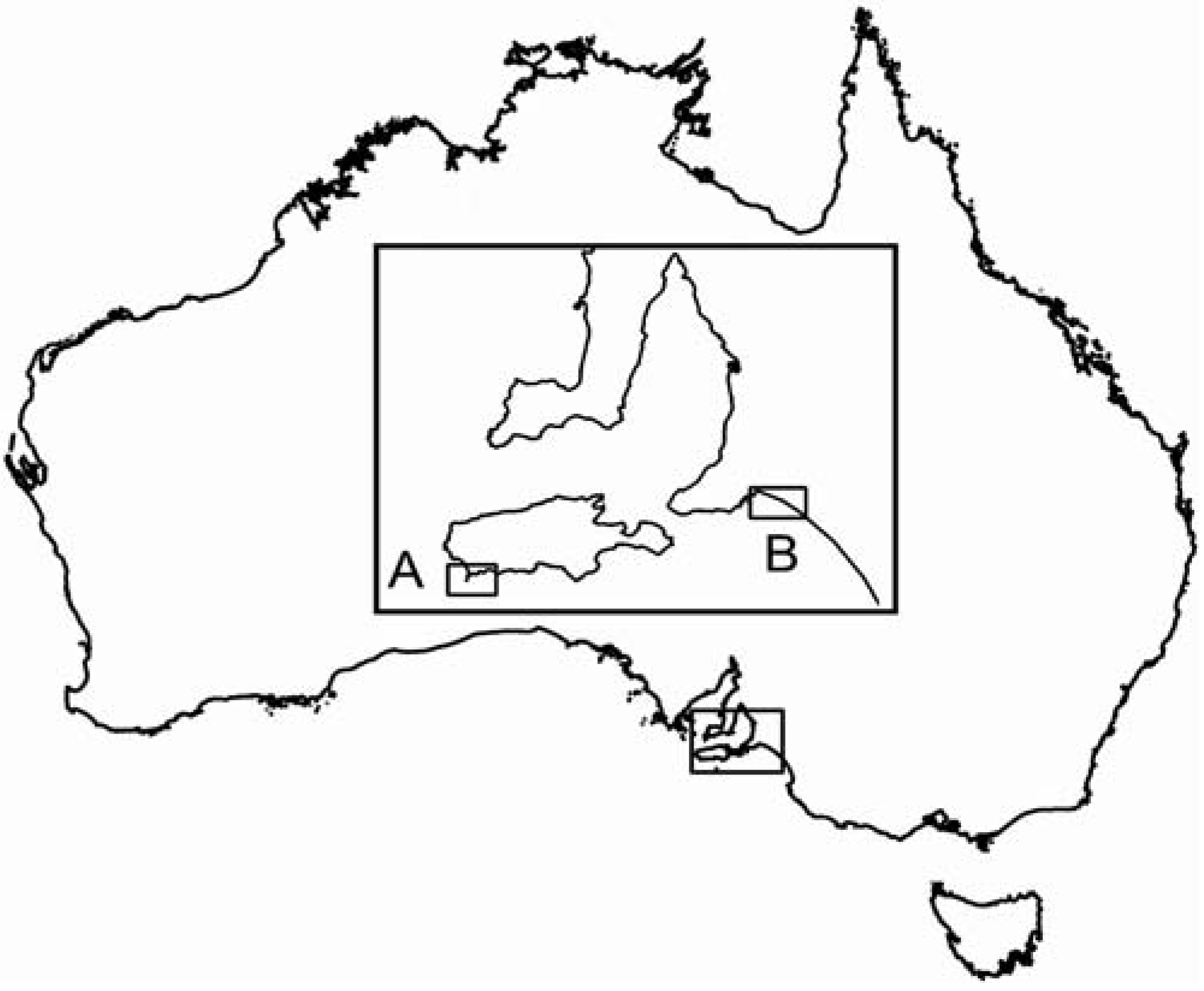
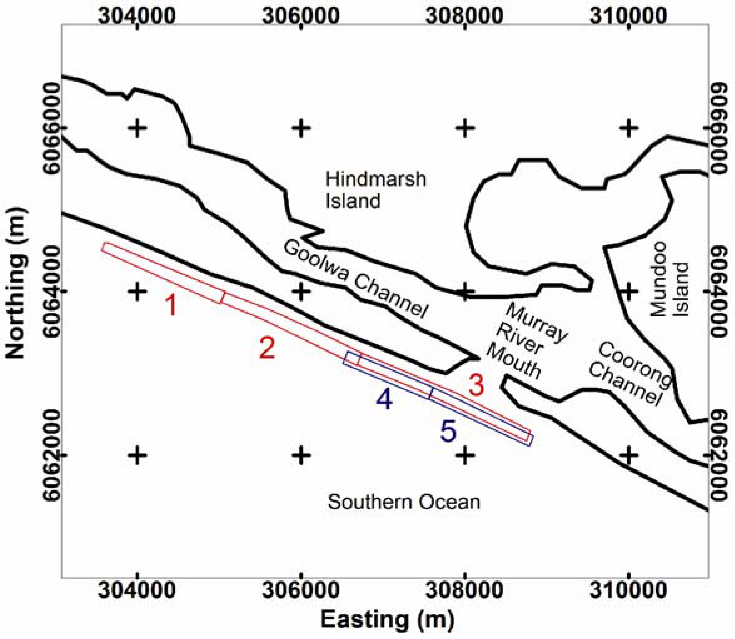
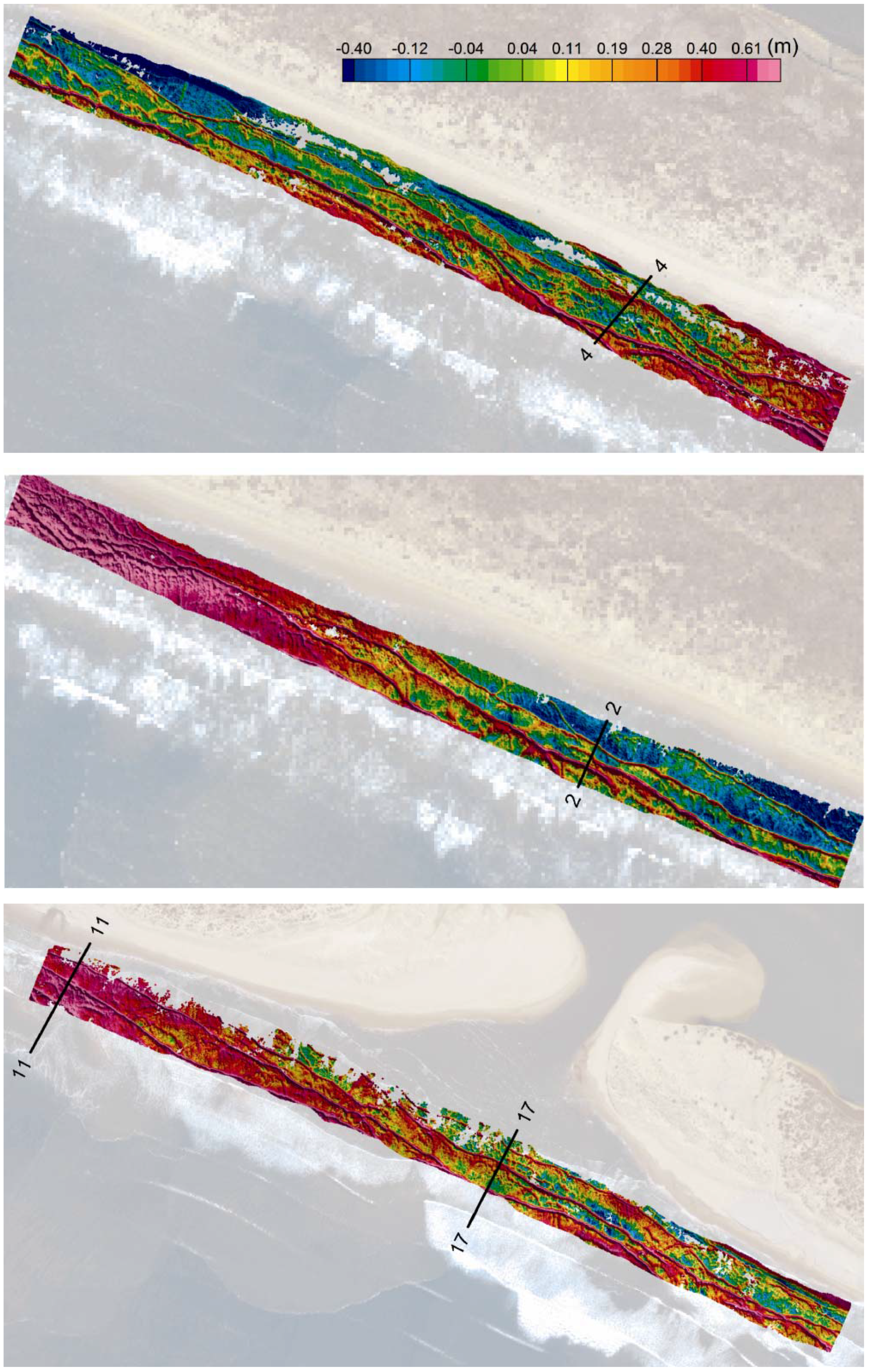
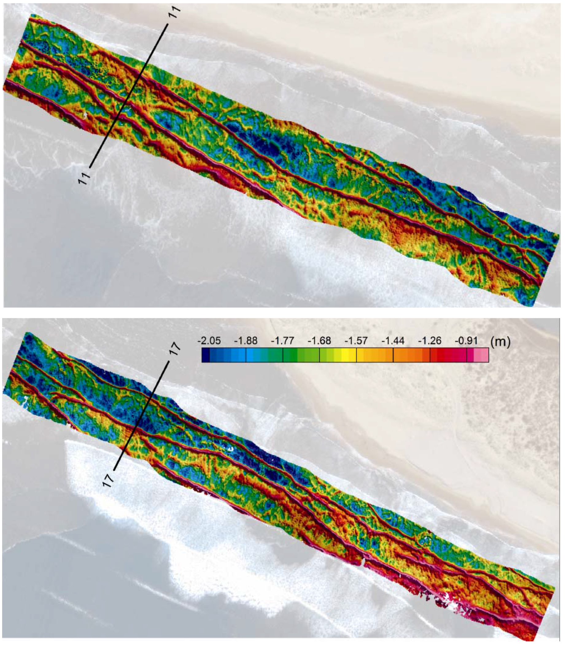
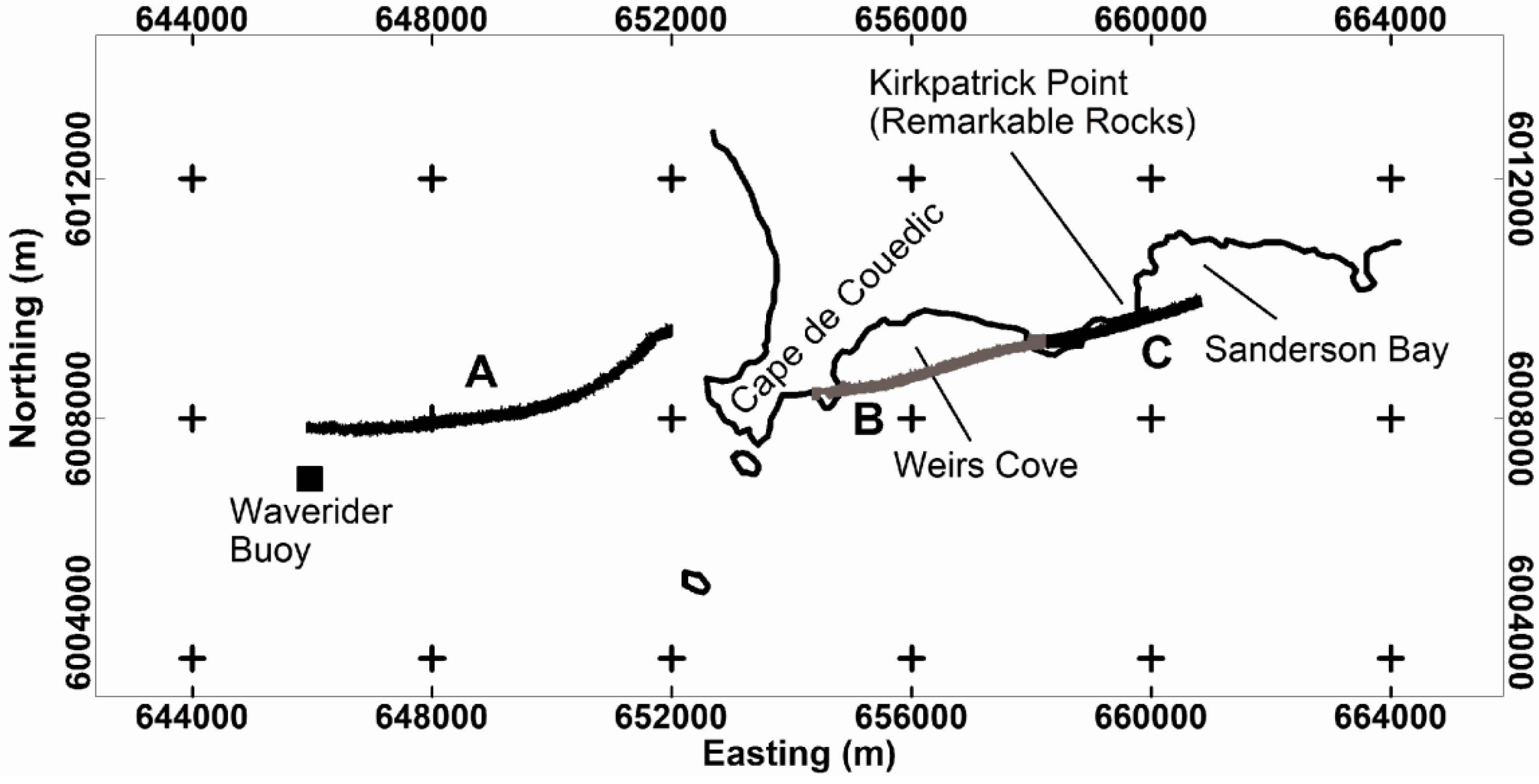
In this study, we evaluated the efficacy of a 2D laser scanner (Riegl model Q240i-80) for measuring the topographic surface of waves in shallow coastal waters and in the surf zone in two study areas shown in Figure 1, the mouth of the Murray River, South Australia (SA) and in surrounding waters of Kangaroo Island, SA, where relative wave heights were compared with wave rider buoy data located near Cape De Couedic on the south-west tip of Kangaroo Island. The Murray River and Cape de Couedic LiDAR surveys were completed in May and June 2007 respectively. A comparison was also made with a second, more complex 2D laser scanner (Riegl model Q560) of significantly higher weight and power supply requirements, simultaneously operating at a longer wavelength with a much higher pulse repetition rate. As this unit has been routinely used and ground-truthed during accurate measurements of terrestrial topographic features [22], its data can be considered to be of benchmark quality for the present study.
We present examples of sea surface topography in both survey areas, using data obtained from a laser scanner operating with a NovAtel/Honeywell GPS-IMU navigation system. We also present similar examples from the mouth of the Murray River survey area using data obtained from: (i) both laser scanners operating simultaneously; and (ii) from one laser scanner operating with two independent navigation systems.
Figure 1. Location of survey areas on Australia’s coastline. Inset: A, Cape de Couedic located on south-west tip of Kangaroo Island (see first figure in Section 3.3 for detail); B, mouth of Murray River area (see first Figure in Section 3.1 for detail).
Remotesensing 03 01983 g001
A similar study was conducted by Reineman et al. [23] in 2008, post-dating our surveys by approximately one year, where a Q240 laser scanner was deployed for ocean and coastal applications, for example: (i) to measure the effects of storm events with regards to beach morphology and erosion; (ii) to determine omnidirectional wavenumber spectrum from sea surface topographic data; and (iii) to measure the wave field around the reef and ocean surrounding a coral island. Whilst there is a degree of overlap between our study and that of Reineman et al. [23], our focus is the comparison of the two LiDAR systems operating simultaneously, over coastal waters and over a surf zone region (to obtain wave profiles) and the use of LiDAR to obtain an altimetry map, which can be used to assist AEM methods for bathymetric mapping by providing an averaged altimetry within an area contained by the larger footprint (relative to the LiDAR system) of the AEM system.

2. Instrumentation

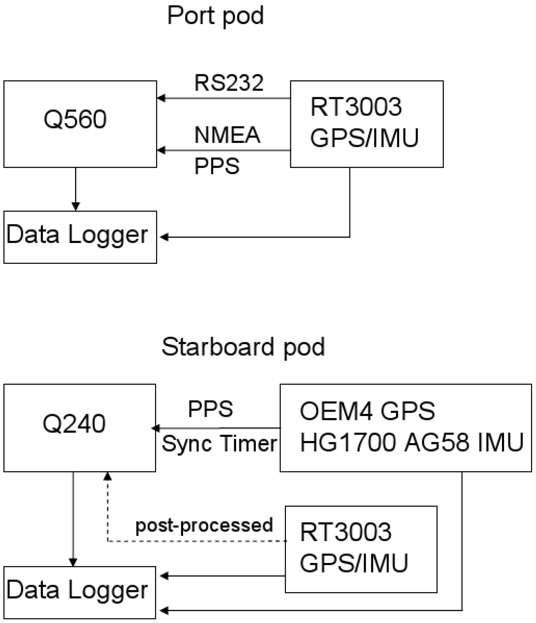
The instrumentation was housed in two pods located on the port and starboard wings of a Diamond HK36TTC -ECO Dimona single-engine aircraft, see Figure 2 and Figure 3. A 2D laser scanner (Riegl model Q240i-80) was mounted within the starboard pod, interfaced to and co-located with a NovAtel SPAN inertial navigation-GPS system (NovAtel OEM4-G2 GPS receiver and Honeywell HG1700 AG58 inertial measurement unit, IMU) co-located with the Q240 scanner. Another GPS-IMU system (OXTS: Oxford Technical Solutions, dual-antenna RT3003 unit) was also co-located with the scanner. This unit contains two NovAtel GPS OEMV receivers, one for each GPS antenna, integrated with a proprietary IMU unit. Temporally synchronized data was acquired from the scanner and the two GPS-IMU systems. The second 2D laser scanner (a full waveform-digitizing Riegl model Q560) was mounted within the port pod, interfaced to and co-located with a second, identical, OXTS RT3003 GPS-IMU system. Temporally synchronized data was acquired from the Q560 scanner and RT3003 unit. The performance of the Q560/RT3003 LiDAR system has been thoroughly demonstrated over terrestrial terrain [24] and is routinely used by Airborne Research Australia (ARA) and others for remote sensing of the environment [22,25,26,27,28].
The focus of this study was to demonstrate the operational functionality and effectiveness of the Q240 and Q560 scanners for measuring sea surface topography and for obtaining wave profiles. The experimental configuration (Figure 2 and Figure 3) allowed a direct comparison of the considerably more expensive Q560 scanner with the Q240 scanner, operating at wavelengths of around 1,500 nm and 1,000 nm respectively, using the same GPS-IMU system (OXTS RT3003), and also a comparison of topographic data obtained from the Q240 scanner using two different GPS-IMU systems.
While the Q240 scanner has a maximum available scan angle range of ±40°, this was set to ±22.5° (start angle 67.5°, angular step 0.18°, 250 shots per line) to match the footprint (as determined by the scan angle) of the Q560 scanner. The pulse repetition rate was set to 30 kHz, which in conjunction with the angular step rate and number of facets of the mirror wheel results in an overall scan rate of about 60 lines/s (resulting in less than 1 m line spacing on the ground at typical survey speeds). As the Q240 is limited to registering and analyzing only one of the many possible returns generated by an outgoing pulse, it was configured to record only the last valid return for each scan step.
The Q560 scanner also was set up for a scan angle of ±22.5° at a line rate of 60 lines/s. Due to the much higher pulse repetition rate of 100 kHz, this results in a much smaller angular step (i.e., the interval between individual samples along the scan line) and thus about 835 laser shots in each scan line. As the Q560 digitizes the full waveform of the receiver signal it does not require any arbitrary restriction to a given return (reflected back from the sea surface).
The set-up of the scanners neglected the wing dihedral angle (3°), thus the central beams of the two scanners are offset by 6° resulting in approximately 40° of overlap between the two fields of view. In order to achieve the best possible quality of post-processed navigation data, the GPS units and inertial systems were configured to record raw data at their highest respective rates (about 2 Hz for GPS measurements and 100 Hz for accelerometers and gyro data).
Figure 2. Experimental set-up on port and starboard wing pods.
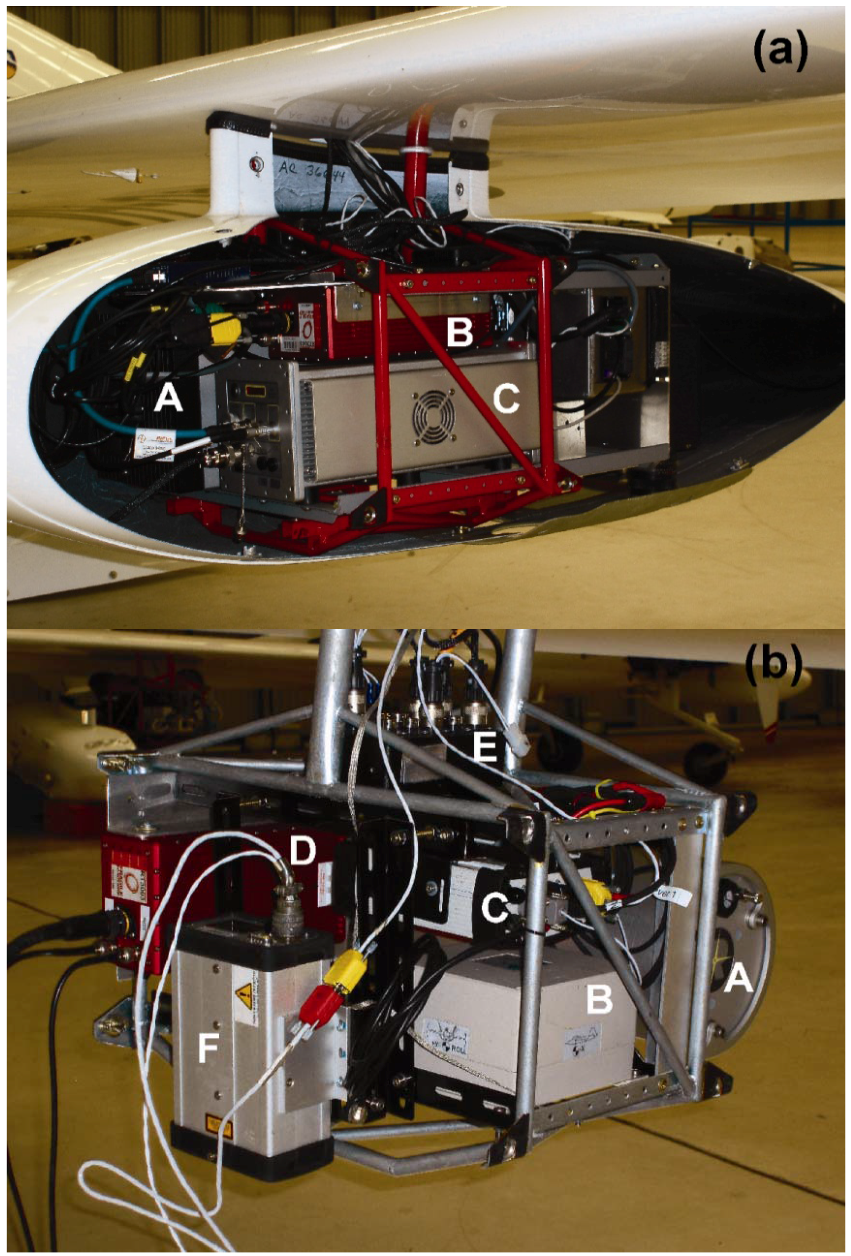
Remotesensing 03 01983 g002
Figure 3. Instrumentation configuration: (a) Port pod assembly: (A), Q560 scanner; (B), RT3003 GPS-IMU; (C), data logger; and (b) Starboard pod assembly: (A), Q240 scanner; (B), HG1700 AG58 IMU; (C), NovAtel OEM4 GPS; (D), RT3003 GPS-IMU; (E), data logger; (F), LD90 altimeter.
Remotesensing 03 01983 g003
The post-processed scanner data provides the altitude (elevation) between the sea surface and the LiDAR which is independent of the GPS height accuracy. This elevation is subtracted from the GPS altitude which is referenced to the WGS84 ellipsoid to determine the instantaneous sea surface topography. Thus the datum of the wave topography is the ellipsoid. While the accuracy of the laser ranging (and hence altimetry) is of the order of cm, the accuracy of the absolute height of the instantaneous sea surface relative to the ellipsoid is determined chiefly by the height accuracy of the GPS data. As the focus of this study was to demonstrate the functionality and effectiveness of the Q240 and Q560 scanners for measuring relative sea surface topography over short time scales (minutes), as opposed to absolute altimetry referenced to a given datum, the use of geoidal GPS data (e.g., using the Australian Height Datum AHD or the EGM96 geoid specifications) was not required, neither was the use of base station differential GPS corrections to improve GPS height accuracy and to remove low frequency drift in the GPS height above the WGS84 ellipsoid. The elevation of the LiDAR system above the sea surface is derived from post-processed data obtained directly from LiDAR measurements and is independent of the GPS altitude. Thus altimetry maps derived from laser scanner data are not affected by GPS errors to the same extent as sea surface topography referenced to the WGS84 ellipsoid datum, and are deemed to be suitable for supporting AEM methodology.
Kinematic differential GPS processing combined with GPS base station data would be required to obtain accurate GPS solutions for the flight trajectories, in particular the vertical GPS height, in order to remove significant low frequency drift that would mask low frequency changes in wave height in coastal areas. Such corrections would be critical, for example, for comparing spatial changes of wave heights over long periods, for obtaining the omnidirectional wavenumber spectrum, and for providing a datum for wave height profiles. In order to proceed from the demonstration phase which is the objective of this study, to more robust applications of LiDAR for studying coastal processes, we recommend normal LiDAR industry practice, i.e., the use of GPS base station corrections, differential kinematic GPS processing and post-processing (e.g., processing with NovAtel’s Waypoint GrafNav and Inertial Explorer software).

System Validation

Initial flight trials over buildings and roads at an altitude range of about 150 to 300 m, confirmed that both scanners were operating correctly. After post-processing/refining the navigation data from all 3 GPS-IMU units using the NovAtel ‘WayPoint’ software package, various comparisons were made: (i) the data from the Q240 scanner, processed either using the NovAtel SPAN or OXTS RT3003 navigation data, resulted in essentially the same 3D topographic accuracy (about 1 m horizontal resolution from 300 m altitude with a vertical jitter of less than 5 cm) based on ground structures with well documented position and altitude that were used as reference targets; (ii) the relative agreement between the Q560 and Q240 scanners, both processed in conjunction with the RT3003 data from the unit mounted in their respective pods, was also likewise estimated to be better than 5 cm for this range of altitudes.
The effect of errors associated with the IMUs on measuring sea surface heights are small compared to GPS errors for the survey altitudes of 150 to 300 m used in this study. Following Reineman et al. [23], the attitude errors can be decomposed as a sum of the mean and fluctuating errors. The mean pitch, roll and azimuth errors are associated with the static alignment offsets between the LiDAR scanner and the IMU and were minimized (by determining the offset constants and minimizing the residuals) during initial flight trials using known ground structures as reference targets. The attitude accuracies (fluctuating errors) of the NovAtel SPAN and the Oxford Technical Solutions RT3003 systems are estimated by the manufacturers to be 0.015° and 0.03° respectively for pitch and roll angles (ξ, θ) and 0.05° and 0.1° respectively for azimuth (yaw, heading) angle (φ). Thus Δθ = Δξ = 0.015° and 0.03° and Δφ = 0.05° and 0.1° for the SPAN and RT3003 systems respectively. The vertical and horizontal position errors arising from the time-varying attitude errors are a function of the swath angle (α) and distance h above the planar surface. Assuming small attitude errors (i.e., within the small angle approximation for trigonometric functions), the vertical position error resulting from the roll error is given by Δ z ( Δ θ ) = h ​   Δ θ tan α ; the horizontal position error resulting from the pitch and roll error is given by Δ x ( Δ ξ ) = h    Δ ξ and Δ y ( Δ θ ) = h    Δ θ respectively; and the horizontal position error Δr resulting from the azimuthal error Δ φ is Δ r ( Δ φ ) = h    Δ φ tan α . Note that the position errors scale linearly with height—thus the class 1 rating of both laser scanners allows deployment at lower altitudes thereby reducing the effects of the fluctuating attitude errors. At the maximum swath angle set to 22.5°, and assuming a flying height of 200 m, the fluctuating errors associated with the RT3003 system are estimated to be Δz = 4.3 cm, Δx = 10.5 cm and Δr = 14.6 cm, and half these values for the SPAN system. These horizontal errors are comparable or smaller than the typical GPS horizontal errors and the vertical errors are smaller than the vertical errors associated with single point GPS positioning (where no differential or base station corrections have been applied) which will be affected by low frequency drift in height accuracy.

3. Results

3.1. Mouth of Murray River Region

The survey was flown over the surf zone consisting of relatively small breaking waves, approximately 1 m in height, as shown in Figure 4. Figure 5 shows the locations of three contiguous segments of processed Q240 data blocks, and two contiguous segments of processed Q560 data blocks, located in the surf zone adjacent to the mouth of the Murray River. Because of the dihedral angle of the wings, there is not complete overlap of the Q240 and Q560 footprints, as seen in Figure 5 (segments 3–5). In this Section, we show a comparison of sea surface topography and wave profiles obtained from Q240 and Q560 data. We also compare the sea surface wave profiles derived from three Q240 datasets—(i) using the NovAtel-Honeywell navigation data with no post-processing; (ii) using RT3003 navigation data with no post processing; and (iii) using RT3003 navigation data with precise point positioning (PPP) processing.
Figure 4. Surf zone, Mouth of the Murray River during the LiDAR survey (10 May 2007). The mouth of the Murray River is located at “X”, the Coorong Channel is located at “Y”.
Remotesensing 03 01983 g004
Figure 5. Mouth of Murray River and Coorong area, South Australia. Flight Sections 1–3: Q240; Sections 4 and 5: Q560 (see text). 2,000 m grid spacing (WGS84, SUTM53).
Remotesensing 03 01983 g005
A section of the sea surface topography in the surf zone adjacent to the mouth of the Murray River is shown in Figure 6 using data obtained from the Q240 scanner and NovAtel-Honeywell navigation system. The interpolation of measured data to a gridded surface, referred to as a “grid” reveals wave heights of up to approximately 1 m and clearly shows the detailed structure of the sea surface. The low frequency drift in GPS altimetry is evident in the upper tile (Section 1, Figure 5) with the wave surface appearing to be inclined left to right by about one meter, giving rise to a grid appearance with a constant color (red) using the color scale in Figure 6. Wave profiles for two transects (Lines 2 and 4, Figure 6) are shown in Figure 7, showing that Q240 LiDAR is capable of resolving relative height variations of approximately 10 cm for this dataset. This estimate of resolution is based on a visual examination of wave profiles obtained from 22 transects. The use of precise point positioning (based on availability of precise GPS orbit and clock data for post-processing single GPS receiver data to achieve decimeter level accuracy [29]) improves the fit between RT3003 and NovAtel-Honeywell data. The RT3003 data shows a tilt (compare red and blue curves in Figure 7), indicating a roll offset error in the equipment configuration.
The sea surface topography obtained from the Q560 data (RT3003—no GPS data post processing) is shown in Figure 8 and the combined two segments (upper and lower panels of Figure 8) can be compared directly with the topography (Q240) shown in the lower panel in Figure 6. (The aerial imagery shown in Figure 6 and Figure 8 was not photographed at the time of the LiDAR surveys.) Apart from the relative bias resulting from GPS altimetry errors in single point positioning data, the topographic grids obtained from both Q240 and Q560 datasets (Figure 6 and Figure 8) show very similar fine structure in the topography of the surf zone, as shown explicitly in the wave profiles for two transects (Lines 11 and 17, Figure 6 and Figure 8), see Figure 9. These two transects are representative of 22 transects examined in the areas confined by panels 2 and 3 in Figure 5. Based on these datasets, the Q240 and Q560 scanners provide very similar relative wave height profiles and topographic grids, and therefore appear to be equally suitable for mapping the sea surface topography including the surf zone.
Figure 6. Three contiguous sections of sea surface topography (Q240-OEM4-HG1700 AG58 IMU data) in the surf zone. Color scale refers to height (m) above ellipsoid and applies to all three images. Top (linear extent ~1,580 m, width ~105 m), middle (linear extent ~1,825 m, width ~150 m) and bottom (linear extent ~1,835 m, width ~155 m) tiles refer to polygons 1, 2, and 3 in Figure 5 respectively.
Remotesensing 03 01983 g006
Figure 7. Sea surface profiles (height (m) above ellipsoid) in surf zone, mouth of Murray River. Left: Line 4 (Figure 6, middle); Right: Line 2 (Figure 6, top). Blue: Q240-OEM4-HG1700 AG58 IMU; green: Q240-RT3003; red: Q240-RT3003 with GPS precise point positioning post-processing.
Remotesensing 03 01983 g007
Figure 8. Two contiguous sections of sea surface topography (Q560-RT3003 data) in the surf zone. Color scale refers to height (m) above ellipsoid and applies to both images. Images top (linear extent ~1,135 m, width ~165 m) and bottom (linear extent ~1,360 m, width ~155 m) refer to polygons 4 and 5 (Figure 5) respectively.
Remotesensing 03 01983 g008
Figure 9. Sea surface profiles (height (m) above ellipsoid) in surf zone, mouth of Murray River. Left panel: Line 11 (Figure 8, top); right panel: Line 17 (Figure 8, bottom). Green: Q560-RT3003; red: Q240-OEM4-HG1700 AG58 IMU. Note the different scales and relative displacements on the vertical axes. The difference in absolute height is caused by different estimates of GPS height in the single point GPS positioning obtained from the two different GPS receivers.
Remotesensing 03 01983 g009

3.2. Altimetry Mapping

The Riegl LD90 laser altimeter has been successfully used for routine AEM surveys over seawater [30] from 2006 onwards and thus altimetry mapping using the Q240 scanner which has the same wavelength as the LD90 altimeter would be expected to be reliable. The altimetry of the Q240 scanner above the sea surface can be averaged over the LiDAR footprint (i.e., product of the along- and cross-flight extent of point densities) determined by the observed swath, scanner operating parameters and flight speed. Thus the elevation at each point along and across the flight direction can be averaged, over a rectangular area defined by the swath (width) and the distance (length) along-flight determined by a given time interval. When used in conjunction with an AEM system, the time interval could be approximately 0.5 to 1 s as the along-flight extent would be comparable to the diameter of the AEM footprint. This averaged altimetry would be expected to provide a more realistic effective altimetry compared to single spot nadir-looking LD90 measurements, especially in areas where the sea surface is non-planar (in areas of ocean swell and in the surf zone). The processing of laser scanner, IMU and GPS data results in the georeferenced altimetry map, i.e., the corrected heights of the 2D scanner data above the sea surface. The (absolute) sea surface topography (referenced to the WGS84 ellipsoid datum) is subsequently obtained by the relatively trivial procedure of subtracting the altimetry (i.e., the elevations of the LiDAR system above the sea surface, over the whole LiDAR footprint) from the GPS height above the ellipsoid. Thus the altimetry map is not influenced by the error in GPS altitude above the ellipsoid, whereas the absolute topography is affected by GPS height errors, although in this case, the relative topography (as shown in a wave profile) measured over short time scales is expected to be accurate because of negligible drift in the GPS height measurement. Any abrupt (high frequency) changes in the measured GPS height would appear as discontinuities along the flight path, which would be clearly identified in the computed topographic grids shown in Figure 6 and Figure 8 (see also third, fifth and sixth figures in Section 3.3).
Figure 10 shows an example of the altimetry map for the equivalent sea surface topography map of the surf zone adjacent to the mouth of the Murray River as shown in Figure 6, top panel (polygon 1, Figure 5). In this example, the altitude of the scanner is decreasing slowly from the south east (bottom-right) at approximately 155 m above sea level (swath ~125 m) to approximately 105 m in the north west (swath ~97 m). The furrows in the altimetry map clearly match the wave crests in the sea surface topography map.
Figure 10. Altimetry map—Height of Q240 LiDAR above the sea surface (see Figure 6 (top panel) for equivalent sea surface topography map); (linear extent ~1,580 m, width ~105 m): covering polygon 1, Figure 5. The color scale bar shows the altitude in meters.
Remotesensing 03 01983 g010

3.3. Cape de Couedic (Kangaroo Island)

Cape de Couedic is located on the south-west tip of Kangaroo Island. A non-directional waverider buoy is located approximately 7.8 km offshore (36.07°S, 136.62°E) in 80 m water depth, see Figure 11. No other waverider buoys were located in the regional vicinity of the coast and as such, a LiDAR survey was specifically planned to include coverage of waters surrounding the waverider buoy. The LiDAR survey was flown across the southern coastline of the island, approaching the Cape and out towards a non-directional waverider buoy, see Figure 11. The waverider buoy data at the time of survey measured a significant wave height and period of about 1.8 m and 11 s respectively, a zero crossing period (mean period of all the waves in a record) of about 7.5 s, and a period at the peak spectral energy swapping between 10 and 13 s. The 10 s swell was estimated to be coming more from the south south-west, and the 13 s swell was estimated to be coming from the south-west, based on barometric chart data (Ray Rice, personal communication, [31]). The two separate swell directions were also observed during flight over these waters. An example of a 10 min sample of the time series data (Figure 12) that overlaps with the time of the LiDAR survey shows relative wave heights (trough-to-crest) ranging typically 0.8 to 1.5 m. Modeling of wave shoaling shows that there is less than a 10% change in wave heights when water depths vary from 80 m down to 40 m (Ray Rice, personal communication, [31]), which is the water depth at the eastern section of the LiDAR survey segment discussed below.
Figure 13 shows a segment of the grid of the sea surface topography obtained from Q240 LiDAR data (Flight Section A, Figure 11) over waters close to the coastline of Cape de Couedic (~40 m depth) extending to waters approximately 750 m north of the waverider buoy. (Very similar topographic grids were obtained from Q560 data.) The 3D wave surface is clearly visible over the swath of approximately 160–200 m. The profile of the sea surface at approximately the mid-point of the grid, extending along the grid, is shown in Figure 14, presenting relative wave heights (trough-to-crest) that vary from ~2 m to ~0.8 m. These relative wave heights are entirely consistent with trough-to-crest wave heights obtained independently from waverider buoy data shown in Figure 12. The low frequency drift in single-point GPS altitude measurements is clearly apparent as a quasi-sinusoidal baseline drift in both the topographic grid (Figure 13) and the profile (Figure 14) where the absolute mean heights are changing from about −9 m to about −7 m along the flight line as shown in Figure 14.
Figure 11. Cape de Couedic, Kangaroo Island, South Australia. Flight Sections A, B, C (see text). The square symbol shows the location of the waverider buoy. 4,000 m grid spacing (WGS84, SUTM53).
Remotesensing 03 01983 g011
Figure 12. Cape de Couedic waverider buoy time series: relative wave height over a 10 min sample.
Remotesensing 03 01983 g012
Figure 13. Section of sea surface topography (Flight Section A, Figure 11), Cape de Couedic, in vicinity of waverider buoy (646,000 mE, 6,007,000 mN, WGS84, SUTM53) located approximately 750 m due south of the south-west edge of the topographic grid. Q240-NovAtel OEM4-Honeywell HG1700 AG58 IMU data. Grid spacing: 500 m. Color scale bar: meters relative to WGS84 ellipsoid. Mean altimetry: 475 m (±17 m standard deviation). Swath: ~ 160–200 m.
Remotesensing 03 01983 g013
Figure 14. Profile of sea surface (relative to WGS84 ellipsoid) along track located approximately midway along the topographic grid shown in Figure 13.
Remotesensing 03 01983 g014
Figure 15 shows an example of the sea surface topography closer to the southern coastline of Kangaroo Island, over waters located between two promontories (Flight Section B, Figure 11). The surface waves are clearly defined and still show a south-westerly swell direction. Figure 16 shows a further example of measured sea surface topography along the adjacent coastline (Flight Section C, Figure 11) with wave refraction clearly evident at the mouth of a small bay (~659,000 mE, Figure 16). Both these examples show the reduced swath over seawater, compared to land, e.g., Figure 16 shows the swath of ~270 m over land reducing to ~185 m over seawater for a survey altitude of 304 m ± 8 m (standard deviation). This observation shows that relatively larger angles of incidence do not necessarily lead to a larger swath over seawater because of larger reflection losses from the sea surface compared to those from land (where there is mixed vegetation and exposed rock/earth).
Figure 15. Section of sea surface topography, Weirs Cove (Flight Section B, Figure 11), between Kirkpatrick Point (Remarkable Rocks) to the east (50 m above sea level), and a headland adjacent to Cape de Couedic to the west (80 m above sea level). Q240 – NovAtel OEM4 – Honeywell HG1700 AG58 IMU data. Datum: WGS84, SUTM53. Grid spacing: 500 m. Color scale bar: meters relative to WGS84 ellipsoid. Mean altimetry: 275 m (±5 m standard deviation). Swath over seawater: ~170 m.
Remotesensing 03 01983 g015
Figure 16. Section of sea surface topography between Kirkpatrick Point (Remarkable Rocks) to the west (50 m above sea level), and Sanderson Bay to the east (Flight Section C, Figure 11). Q240-HG1700 AG58 IMU data. Datum: WGS84, SUTM53. Grid spacing: 500 m. Color scale bar: meters relative to WGS84 ellipsoid. Mean altimetry over seawater: 304 m (±8 m standard deviation).
Remotesensing 03 01983 g016

4. Conclusions

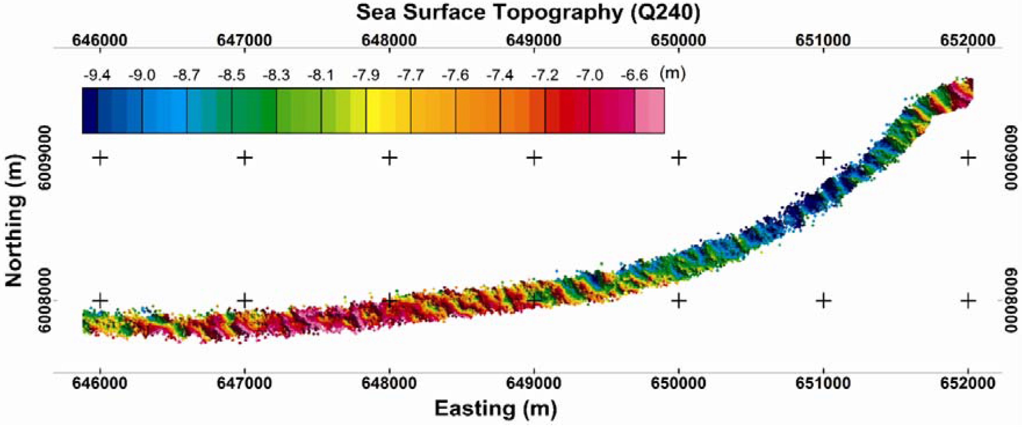
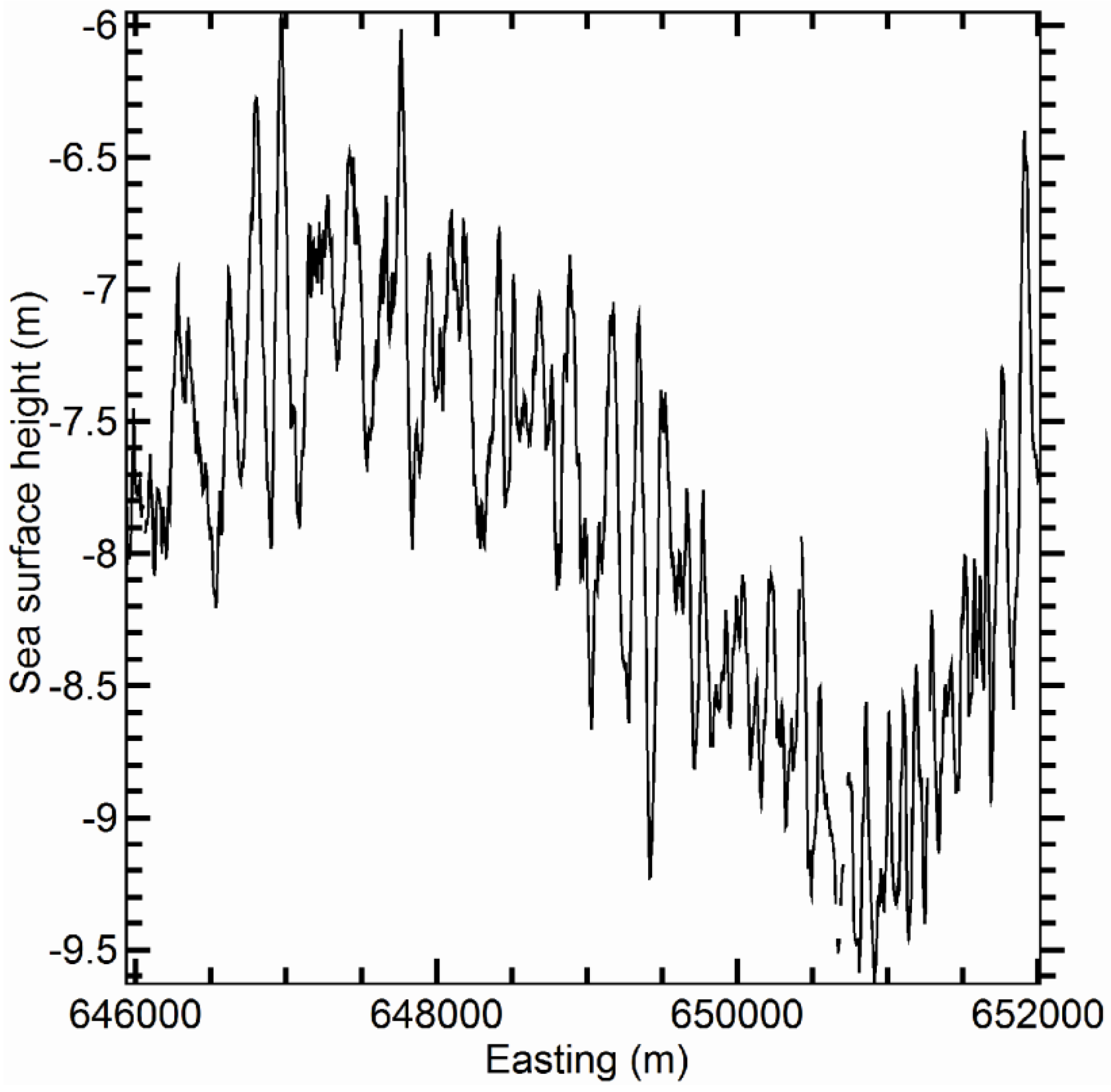
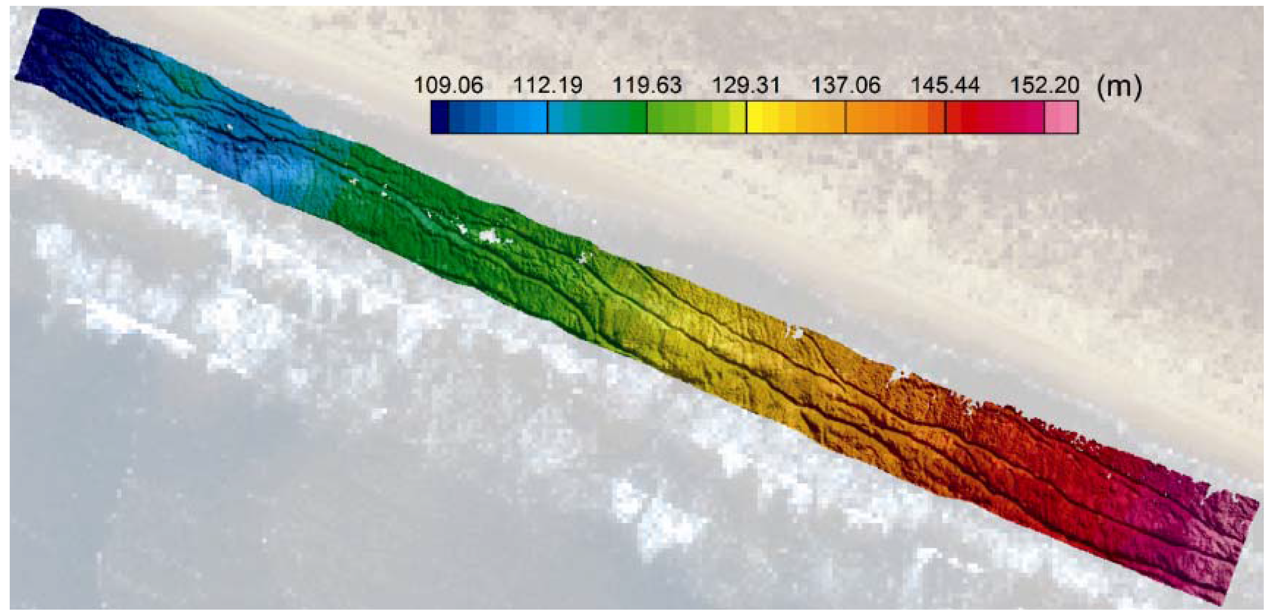
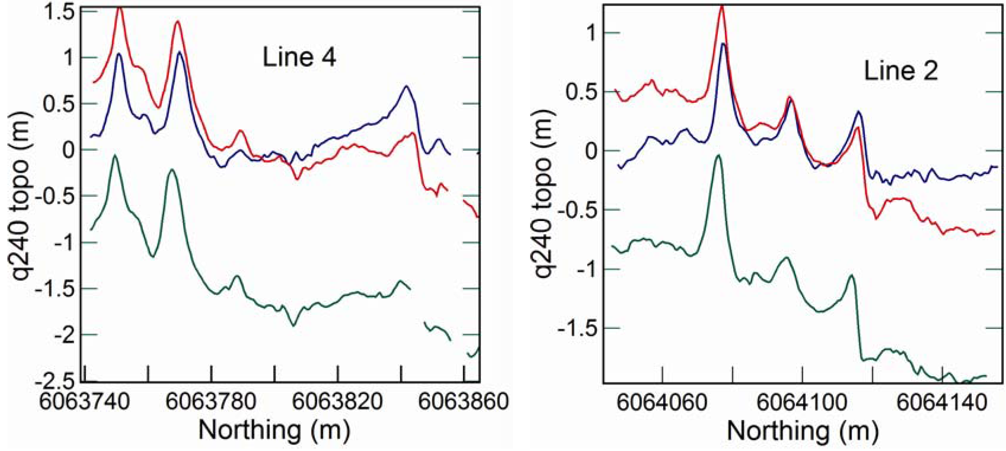
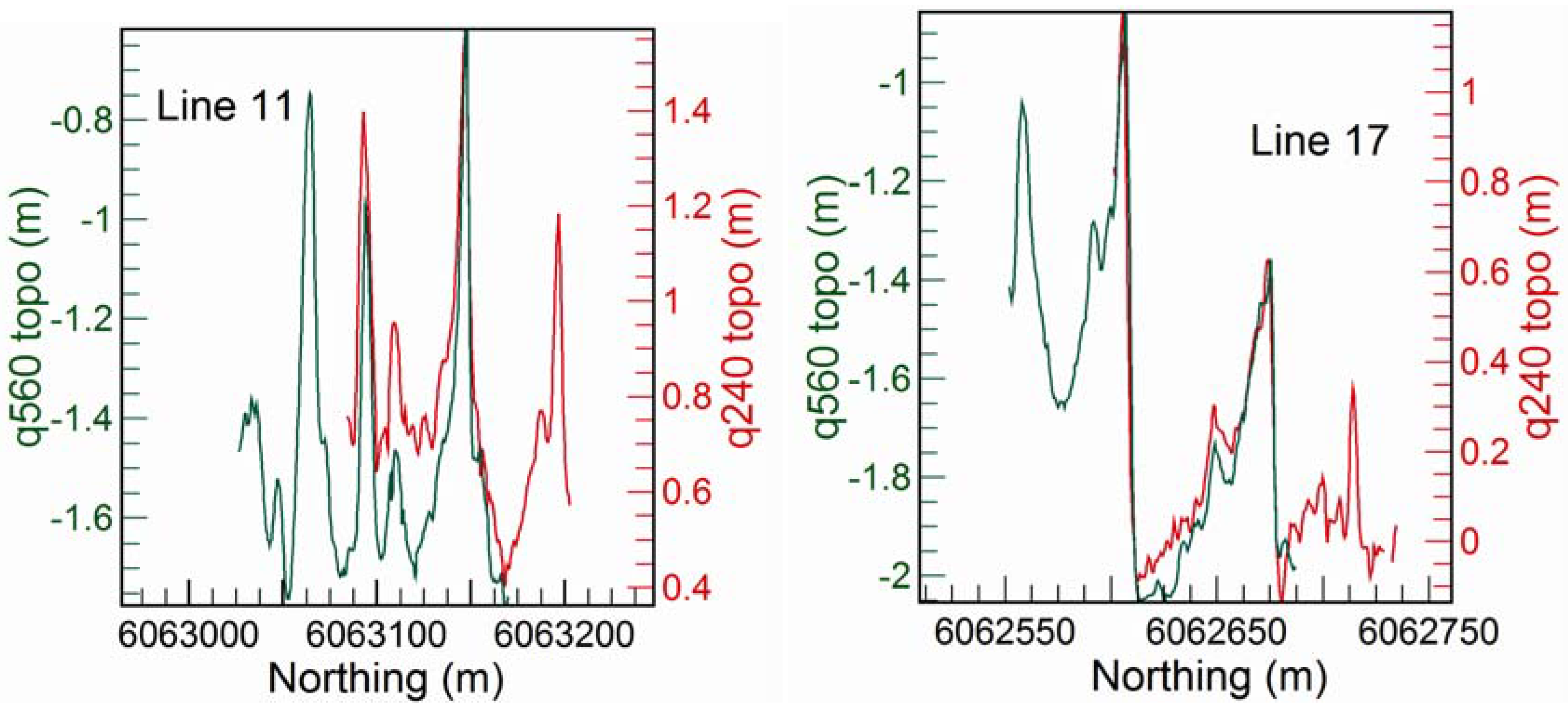
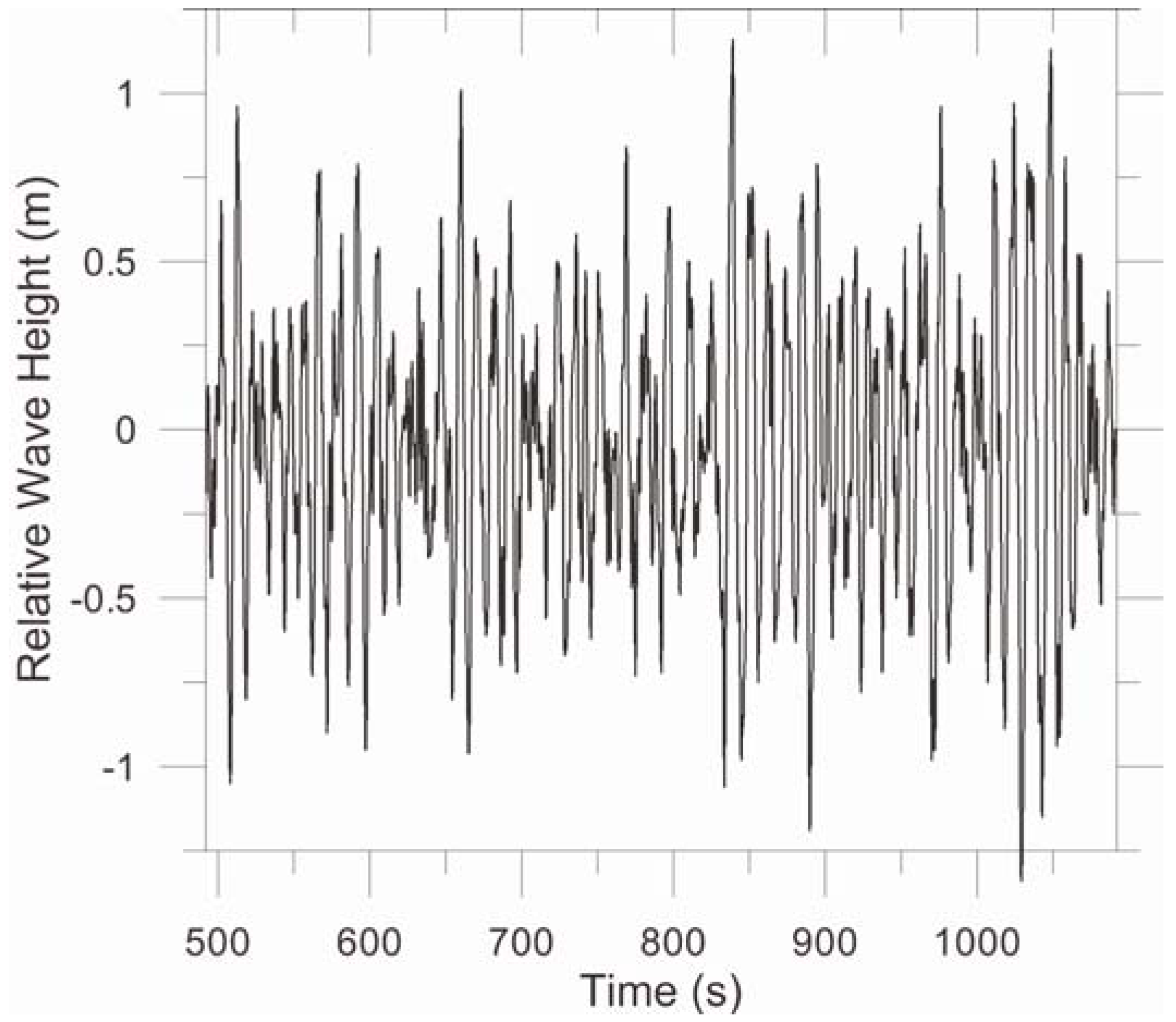
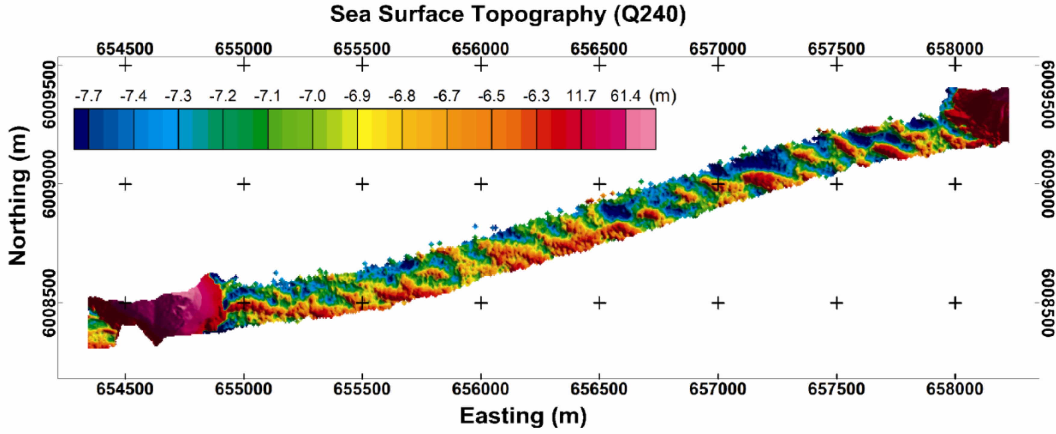
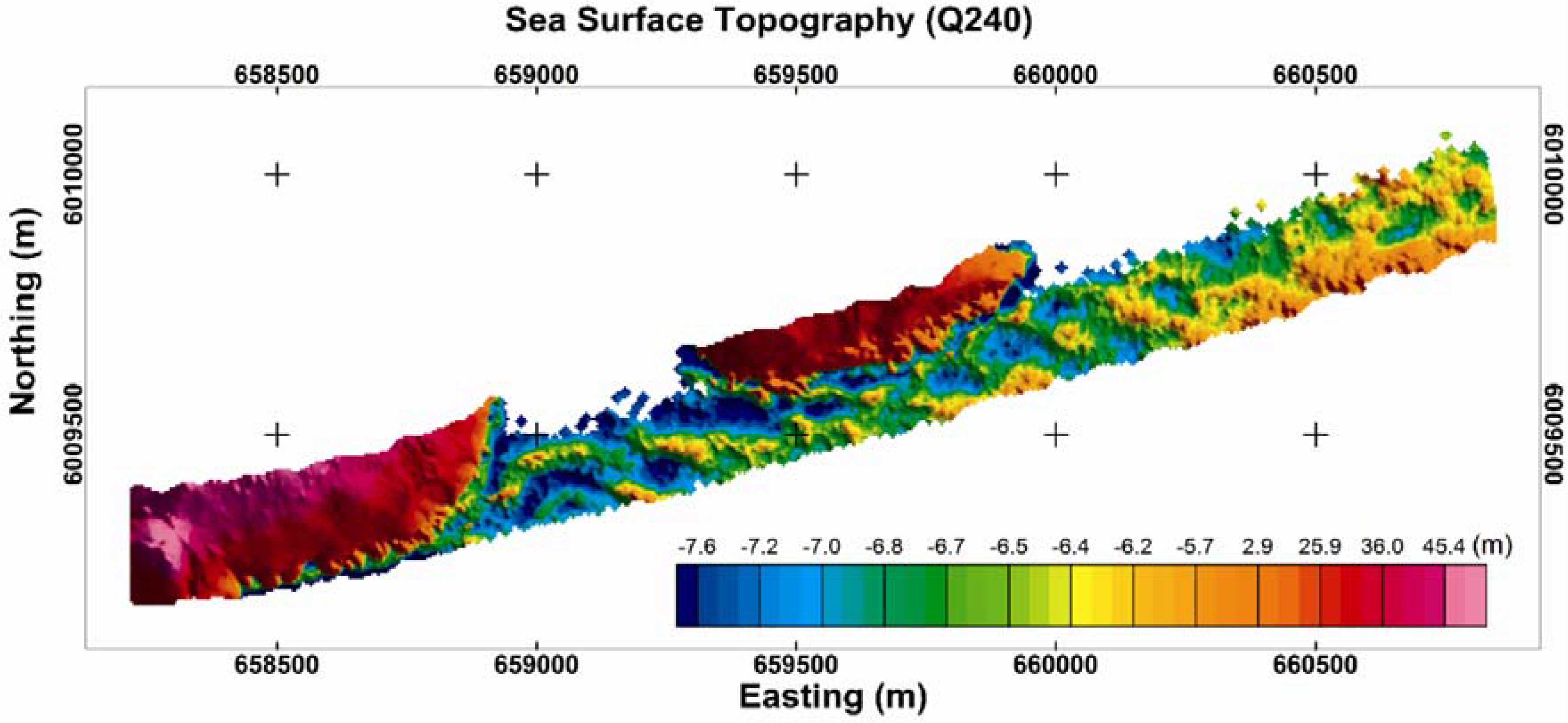
The sea surface topography in coastal waters adjacent to Cape de Couedic, Kangaroo Island (South Australia) and in the surf zone in waters adjacent to the mouth of the Murray River (South Australia) was successfully mapped using two 2D laser scanners (referred to as Q240 and Q560), giving wave profiles that resolve relative height variations of approximately 10 cm. The data for both scanners were recorded simultaneously, mounted on the same aircraft (i.e., the data was measured in a common reference frame), thereby allowing a comparison of the two scanners, which operate at different wavelengths. Both scanners performed equally well in resolving the fine structure of wave profiles. The relative wave heights recorded by the scanners were shown to be consistent with relative wave heights recorded by a waverider buoy in the vicinity of Cape de Couedic.
One potential application of LiDAR over the sea surface is to act as an auxiliary sensor to support the use of airborne electromagnetic methods for bathymetric mapping. The sea surface topography in areas of significant swell could be used for 2D/3D modeling of the electromagnetic response rather than assuming a planar conductive sea surface. Additionally, the processed LiDAR data (prior to subtracting the GPS altitude to determine the sea surface topography) provide altimetry maps which can be subsequently averaged over suitable areas compatible with the electromagnetic footprint to determine an effective altimetry which would be expected to be more reliable that single spot nadir-looking altimeter data.
Based on topographic grids obtained over a range of altitudes, we observed that the Q240 scanner is most suitable for scanning seawater topography from an altitude of about 160–200 m. The limit of obtaining useful reflections from the sea surface is determined by the incidence angle of the laser scanner at the water surface and not by the scan angle (aperture range). Thus scanning at a higher altitude with a narrower aperture can provide a larger useable swath than scanning at a lower altitude with a larger aperture (larger incidence angle). Approximately the same swath can be achieved with the Q560 for water surfaces, but the return reflections require significantly more filtering to remove echoes from foam and spray; there is also occasional loss of returns from the sea surface when the laser penetrates the water column.

Acknowledgments

We thank Gareth Carpenter, South Australian Water Corporation, for providing the aerial imagery used in Figure 6, Figure 8 and Figure 10. J.V. also acknowledges Scott Tremethick, Bureau of Meteorology, South Australia and Ray Rice, Cardino Lawson Treloar Pty Ltd, for the waverider buoy data. We thank four anonymous reviewers for their helpful and constructive suggestions.

References

  1. Guenther, G.C.; Lillycrop, W.J.; Banic, J.R. Future advancements in airborne hydrography. Int. Hydrogr. Rev. 2002, 3, 67–90. [Google Scholar]
  2. Irish, J.L.; Lillycrop, W.J. Scanning laser mapping of the coastal zone: The SHOALS system. ISPRS J. Photogramm. 1999, 54, 123–129. [Google Scholar] [CrossRef]
  3. Smith, W.H.F.; Sandwell, D.T. Global sea floor topography from dense satellite altimetry and sparse shipboard bathymetry. Science 1997, 277, 1956–1962. [Google Scholar] [CrossRef]
  4. Vandemark, D.; Mourad, P.D.; Bailey, S.A.; Crawford, T.L.; Vogel, C.A.; Sun, J.; Chapron, B. Measured changes in ocean surface roughness due to atmospheric boundary layer rolls. J. Geophys. Res. 2001, 106, 4639–4654. [Google Scholar] [CrossRef]
  5. Sun, J.; Burns, S.P.; Vandemark, D.; Donelan, M.A.; Mahrt, L.; Crawford, T.L.; Herbers, T.H.C.; Crescenti, G.H.; French, J.R. Measurements of directional wave spectra using aircraft laser altimeters. J. Atmos. Ocean. Technol. 2005, 22, 869–885. [Google Scholar] [CrossRef]
  6. Schule, J.J.; Simpson, L.S.; DeLeonibus, P.S. A study of fetch-limited wave spectra with an airborne laser. J. Geophy. Res. 1971, 76, 4160–4171. [Google Scholar] [CrossRef]
  7. Krabill, W.; Thomas, R.; Jezek, K.; Kuivinen, K.; Manizade, S. Greenland ice sheet thickness measured by laser altimetry. Geophys. Res. Lett. 1995, 22, 2341–2344. [Google Scholar] [CrossRef]
  8. Hwang, P.A.; Walsh, E.J.; Krabill, W.B.; Swift, R.N.; Manizade, S.S.; Scott, J.F.; Earle, M.D. Airborne remote sensing applications to coastal wave research. J. Geophys. Res. 1998, 103, 18791–18800. [Google Scholar] [CrossRef]
  9. Hwang, P.A.; Krabill, W.B.; Wright, W.; Swift, R.N.; Walsh, E.J. Airborne scanning Lidar measurement of ocean waves. Remote Sens. Environ. 2000, 73, 236–246. [Google Scholar] [CrossRef]
  10. Hwang, P.A.; Wang, D.W.; Walsh, E.J.; Krabill, W.B.; Swift, R.N. Airborne measurements of the wavenumber spectra of ocean surface waves. Part I: Spectral slope and dimensionless spectral coefficient. J. Phys. Ocean. 2000, 30, 2753–2767. [Google Scholar] [CrossRef]
  11. Hwang, P.A.; Wang, D.W.; Walsh, E.J.; Krabill, W.B.; Swift, R.N. Airborne measurements of the wavenumber spectra of ocean surface waves. Part II: Directional distribution. J. Phys. Ocean. 2000, 30, 2753–2767. [Google Scholar] [CrossRef]
  12. Melville, W.K.; Romero, L.; Kleiss, J.M.; Swift, R.N. Extreme wave events in the Gulf of Tehuantepec. In Proceedings of the 14th Aha Huliko’a Hawaiian Winter Workshop on Rogue Waves, Honolulu, HI, USA, 24–28 January 2005; pp. 23–28.
  13. Romero, L.; Melville, W.K. Airborne observations of fetch-limited waves in the Gulf of Tehuantepec. J. Phys. Ocean. 2010, 40, 441–465. [Google Scholar] [CrossRef]
  14. Stockdon, H.; Sallenger, A.; List, J.; Holman, R. Estimation of shoreline position and change using airborne topographic lidar data. J. Coast. Res. 2002, 18, 502–513. [Google Scholar]
  15. Sallenger, A.; Krabill, W.; Brock, J.; Swift, R.; Manizade, S.; Stockdon, H. Sea-cliff erosion as a function of beach changes and extreme wave runup during the 1997–1998 El Nino. Mar. Geol. 2002, 187, 279–297. [Google Scholar] [CrossRef]
  16. Rosser, N.J.; Petley, D.N.; Lim, M.; Dunning, S.A.; Allison, R.J. Terrestrial laser scanning for monitoring the process of hard rock coastal cliff erosion. Q. J. Eng. Geol. Hydrogeol. 2005, 38, 363–375. [Google Scholar] [CrossRef]
  17. Vrbancich, J. Airborne electromagnetic bathymetry investigations in Port Lincoln, South Australia—Comparison with an equivalent floating transient electromagnetic system. Explor. Geophys. 2011. accepted. [Google Scholar] [CrossRef]
  18. Spies, B.; Fitterman, D.; Holladay, S.; Liu, G. (Eds.) Airborne electromagnetics. Explor. Geophys. 1998, 29, 1–271.
  19. Palacky, G.J.; West, G.F. Airborne electromagnetic methods. In Electromagnetic Methods in Applied Geophysics: Applications Part B; Nabighian, M.N., Ed.; Society of Exploration Geophysicists: Tulsa, OK, USA, 1991; pp. 811–879. [Google Scholar]
  20. Vrbancich, J. An investigation of seawater and sediment depth using a prototype airborne electromagnetic instrumentation system—A case study in Broken Bay, Australia. Geophys. Prospect. 2009, 57, 633–651. [Google Scholar] [CrossRef]
  21. Reid, J.E.; Vrbancich, J. A comparison of the inductive-limit footprints of airborne electromagnetic configurations. Geophysics 2004, 69, 1229–1239. [Google Scholar] [CrossRef]
  22. Hacker, J.M.; Lieff, W.; Bannehr, L. Combining Full Wave-Form Laser Scanning, Hyper-spectral Scanning and Other Remote Sensing and in situ Instrumentation on a Small and Environmentally Friendly Airborne Platform: Technology and some Examples from Recent Surveys. In Proceedings of the 14th Australasian Remote Sensing and Photogrammetry Conference, Spatial Sciences Institute Australia, Darwin, Australia, 29 September–3 October 2008.
  23. Reineman, B.D.; Lenain, L.; Melville, W.K. A portable airborne scanning Lidar system for ocean and coastal applications. Atmos. Ocean. Technol. 2009, 26, 2626–2641. [Google Scholar] [CrossRef]
  24. Le, P. Airborne Laser Scanning Accuracy and Precision Over Terrestrial Environments. Honours Thesis, School of Natural and Built Environments, Division of Information Technology, Engineering and the Environment, University of South Australia, Adelaide, SA, Australia, 2007. [Google Scholar]
  25. Lieff, W.; Hacker, J.M.; Ewenz, C.M. Land Surface Characterization Using LIDAR Data. In Proceedings of the 14th National AMOS Conference, Adelaide, SA, Australia, 5–8 February 2007; p. 33.
  26. Dashti, M. Individual Tree Mapping and Classification Using High Density Airborne Lidar. Honours Thesis, School of Natural and Built Environments, Division of Information Technology, Engineering and the Environment, University of South Australia, Adelaide, SA, Australia, 2010. [Google Scholar]
  27. Bertels, L.; Houthys, R.; Sterckx, S.; Knaeps, E.; Deronde, B. Large-scale mapping of the riverbanks, mud flats and salt marshes of the Scheldt basin using airborne imaging spectroscopy and LiDAR. Int. J. Remote Sens. 2011, 32, 2905–2918. [Google Scholar] [CrossRef]
  28. Lasaponara, R.; Masini, N. Full-waveform airborne laser scanning for the detection of medieval archaeological microtopographic relief. J. Cult. Herit. 2009, 10, e78–e82. [Google Scholar] [CrossRef]
  29. Bisnath, S.; Gao, Y. Precise point positioning. GPS World 2009, 20, 43–50. [Google Scholar]
  30. Kratzer, T.; Vrbancich, J. Real-time kinematic tracking of towed AEM birds. Explor. Geophys. 2007, 38, 132–143. [Google Scholar] [CrossRef]
  31. Rice, R.; Cardino Lawson Treloar Pty Ltd. Personal communication, 2007.

