Environmental and Sensor Limitations in Optical Remote Sensing of Coral Reefs: Implications for Monitoring and Sensor Design


Abstract
:
1. Introduction
2. Methods
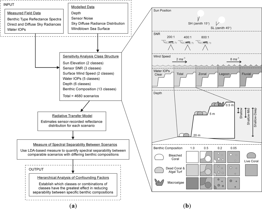
2.1. Overview
2.2. Sensitivity Analysis Structure
2.3. Radiative Transfer Model
2.4. Measure of Spectral Separability between Scenarios
2.5. Hierarchical Analysis of Confounding Factors
3. Results and Discussion
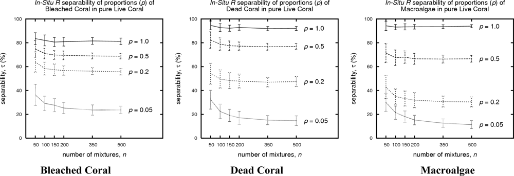
3.1. In situ Spectral Separabilities of Benthic Classes
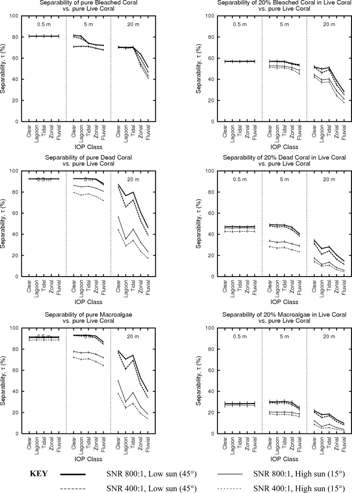
3.2. Individual Effect of Environmental and Sensor Factors
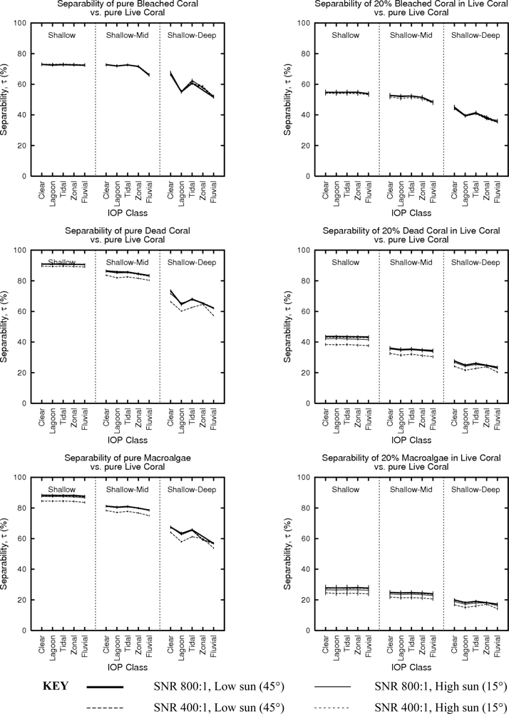
3.3. Effect of Variation in Depth vs. Absolute Depth
3.4. Effect of Variation in IOP Values vs.Absolute IOP Values
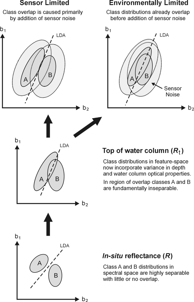
3.5. Sensor-Noise Limited vs. Environmentally Limited Scenarios
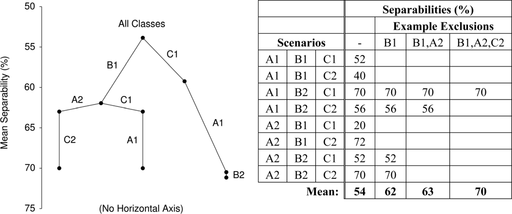
3.6. Hierarchical Analysis of Confounding Factors
3.6.1. Initial Factor Exclusion—Sub-Pixel Proportions
3.6.2. Second Tier—Water Depth and Sun Position
3.6.3. High Accuracy Plateau—Insignificant Factors
4. Conclusions
Acknowledgments
References
- Elvidge, C.D.; Dietz, J.B.; Berklemans, R.; Andréfouët, S.; Skirving, W.; Strong, A.E.; Tuttle, B.T. Satellite observation of Keppel Islands (Great Barrier Reef) 2002 coral bleaching using IKONOS data. Coral Reefs 2004, 23, 123–132. [Google Scholar]
- Mumby, P.J.; Chisholm, J.R.M.; Clark, C.D.; Hedley, J.D.; Jaubert, J. A bird’s eye view of the health of coral reefs. Nature 2001, 413, 36. [Google Scholar]
- Mumby, P.J.; Hedley, J.D.; Chisholm, J.R.M.; Clark, C.D.; Ripley, H.; Jaubert, J. The cover of living and dead corals from airborne remote sensing. Coral Reefs 2004, 23, 171–183. [Google Scholar]
- Hedley, J.D.; Mumby, P.J. Biological and remote sensing perspectives of pigmentation in coral reef organisms. Adv. Mar. Biol 2002, 43, 277–317. [Google Scholar]
- Lesser, M.P.; Mobley, C.D. Bathymetry, water optical properties, and benthic classification of coral reefs using hyperspectral remote sensing imagery. Coral Reefs 2007, 26, 819–829. [Google Scholar]
- Hochberg, E.J.; Atkinson, M.J.; Andréfouët, S. Spectral reflectance of coral reef bottom types worldwide and implications for coral reef remote sensing. Remote Sens. Environ 2003, 85, 159–173. [Google Scholar]
- Hochberg, E.J.; Atkinson, M.J. Capabilities of remote sensors to classify coral, algae and sand as pure and mixed spectra. Remote Sens. Environ 2003, 85, 174–189. [Google Scholar]
- Karpouzli, E.; Malthus, T.J.; Place, C.J. Hyperspectral discrimination of coral reef benthic communities in the western Caribbean. Coral Reefs 2004, 23, 141–151. [Google Scholar]
- Kutser, T.; Dekker, A.G.; Skirving, W. Modeling spectral discrimination of Great Barrier Reef benthic communities by remote sensing instruments. Limnol. Oceanogr 2003, 48, 497–510. [Google Scholar]
- Lubin, D.; Li, W.; Dustan, P.; Mazel, C.H.; Stamnes, K. Spectral Signatures of coral reefs: Features from space. Remote Sens. Environ 2001, 75, 127–137. [Google Scholar]
- Malthus, T.; Mumby, P.J. Remote sensing of the coastal zone: An overview and priorities for future research. Int. J. Remote Sens 2003, 24, 2805–2815. [Google Scholar]
- Phinn, S.R.; Dekker, A.G.; Brando, V.E.; Roelfsema, C.M. Mapping water quality and substrate cover in optically complex coastal and reef waters: An integrated approach. Mar. Pollut. Bull 2005, 51, 459–469. [Google Scholar]
- Hedley, J.D.; Mumby, P.J.; Joyce, K.E.; Phinn, S.R. Spectral unmixing of coral reef benthos under ideal conditions. Coral Reefs 2004, 23, 60–73. [Google Scholar]
- Hedley, J.D.; Mumby, P.J. A remote sensing method for resolving depth and subpixel composition of aquatic benthos. Limnol. Oceanogr 2003, 48, 480–488. [Google Scholar] [Green Version]
- Lee, Z.P.; Carder, K.L.; Mobley, C.D.; Steward, R.G.; Patch, J.S. Hyperspectral remote sensing for shallow waters, 1. A semi-analytical model. Appl. Opt 1998, 37, 6329–6338. [Google Scholar]
- Lee, Z.P.; Carder, K.L.; Mobley, C.D.; Steward, R.G.; Patch, J.S. Hyperspectral remote sensing for shallow waters, 2. Deriving bottom depths and water properties by optimization. Appl. Opt 1999, 38, 3831–3843. [Google Scholar]
- Lee, Z.; Carder, K.L.; Chen, R.F.; Peacock, T.G. Properties of the water column and bottom derived from Airborne Visible Infrared Imaging Spectrometer (AVIRIS) data. J. Geophys. Res 2001, 106, 11639–11651. [Google Scholar]
- Mobley, C.D.; Sundman, L.K.; Davis, C.O.; Bowles, J.H.; Downes, T.V.; Leathers, R.A.; Montes, M.J.; Bisset, W.P.; Kohler, D.D.R.; Reid, R.P.; Louchard, A.M.; Gleason, A. Interpretation of hyperspectral remote-sensing imagery by spectrum matching and look-up tables. Appl. Opt 2005, 44, 3576–3592. [Google Scholar]
- Brando, V.E.; Anstee, J.M.; Wettle, M.; Dekker, A.G.; Phinn, S.R.; Roelfsema, C. A physics based retrieval and quality assessment of bathymetry from suboptimal hyperspectral data. Remote Sens. Environ 2009, 113, 755–770. [Google Scholar]
- Hedley, J.D.; Roelfsema, C.M.; Phinn, S.R. Efficient radiative transfer model inversion for remote sensing applications. Remote Sens. Environ 2009, 113, 2527–2532. [Google Scholar]
- Dekker, A.G.; Phinn, S.R.; Anstee, J.; Bissett, P.; Brando, V.E.; Casey, B.; Fearns, P.; Hedley, J.; Klonowski, W.; Lee, Z.P.; Lynch, M.; Lyons, M.; Mobley, C.; Roelfsema, C. Intercomparison of shallow water bathymetry, hydro-optics, and benthos mapping techniques in Australian and Caribbean coastal environments. Limnol. Oceanogr. Methods 2011, 9, 396–425. [Google Scholar]
- Green, E.P.; Mumby, P.J.; Edwards, A.J.; Clark, C.D. Remote Sensing Handbook for Tropical Coastal Management; UNESCO: Paris, France, 2000. [Google Scholar]
- Mobley, C.D. Thematic mapping. Ocean Optics Web Book. 2012. Available online: http://www.oceanopticsbook.info/view/remote_sensing/level_2/thematic_mapping (accessed on 20 January 2012).
- Mobley, C.D.; Sundman, L.K. Effects of optically shallow waters on upwelling radiances: Inhomogeneous and sloping bottoms. Limnol. Oceanogr 2003, 48, 329–336. [Google Scholar]
- Grant, R.H.; Hiesler, G.M.; Gao, W. Photosynthetically-active radiation: Sky radiance distributions under clear and overcast conditions. Agric. For. Meteorol 1996, 82, 267–292. [Google Scholar]
- Cox, C.; Munk, W. Statistics of the sea surface derived from sun glitter. J. Mar. Res 1954, 13, 198–227. [Google Scholar]
- Mobley, C.D. Light and Water; Academic Press: San Diego, CA, USA, 1994. [Google Scholar]
- Mather, P.M. Computer Processing of Remotely-Sensed Images, 2nd ed.; Wiley: New York, NY, USA, 1999. [Google Scholar]
- Lucas, R.; Rowlands, A.; Niemann, O.; Merton, R.N. Hyperspectral sensors and applications. In Advanced Image Processing Techniques for Remote Sensed Hyperspectral Data; Varshney, P.K., Arora, M.J., Eds.; Springer-Verlag: New York, NY, USA, 2004; pp. 11–49. [Google Scholar]
- Roelfsema, C.M.; Marshall, J.; Hochberg, E.; Phinn, S.; Goldizen, A.; Joyce, K. Underwater Spectrometer System 2004 (UWSS04); Centre for Remote Sensing and Spatial Information Science, University of Queensland: Brisbane, QLD, Australia, 2006. [Google Scholar]
- Hedley, J. A three-dimensional radiative transfer model for shallow water environments. Opt. Express 2008, 16, 21887–21902. [Google Scholar]
- Mobley, C.D.; Sundman, L.K. Hydrolight 4.1 Users’ Guide; Sequoia Scientific Inc.: Redmond, WA, USA, 2000. [Google Scholar]
- Hedley, J.D.; Harborne, A.R.; Mumby, P.J. Simple and robust removal of sun glint for mapping shallow water benthos. Int. J. Remote Sens 2005, 26, 2107–2112. [Google Scholar]
- Mueller, J.L. Ocean Optics Protocols for Satellite Ocean Color Sensor Validation; NASA/TM 2003-211621/Rev 4-Vol IV (Erratum 1); 2003. [Google Scholar]
- Smith, R.C.; Baker, K.S. Optical properties of the clearest natural waters (200–800 nm). Appl. Opt 2001, 20, 177–184. [Google Scholar]
- Boss, E.; Pegau, W.S. Relationship of light scattering at an angle in the backward direction to the backscattering coefficient. Appl. Opt 2001, 40, 5503–5507. [Google Scholar]
- Mobley, C.D.; Sundman, L.K.; Boss, E. Phase function effects on oceanic light fields. Appl. Opt 2002, 41, 1035–1050. [Google Scholar]
- Karpouzli, E.; Malthus, T.; Place, C.; Mitchell Chui, A.; Ines Garcia, M.; Mair, J. Underwater light characterisation for correction of remotely sensed images. Int. J. Remote Sens 2003, 24, 2683–2702. [Google Scholar]
- Tabachnick, B.G.; Fidell, L.S. Using Multivariate Statistics, 4th ed.; Allyn and Bacon: London, UK, 2001. [Google Scholar]
- Ma, Z.; Redmond, R.L. Tau coefficients for accuracy assessment of classification of remotely sensed data. Photogramm. Eng. Remote Sensing 1995, 61, 435–439. [Google Scholar]
- Sokal, R.R.; Rohlf, F.J. Biometry, 3rd ed.; Freeman: San Francisco, CA, USA, 1995. [Google Scholar]
- Christofides, N. Graph theory. An algorithmic approach; Academic Press: London, UK, 1975. [Google Scholar]
- Leiper, I.A.; Siebeck, U.E.; Marshall, N.J.; Phinn, S.R. Coral health monitoring: Linking coral colour and remote sensing techniques. Can. J. Remote Sensing 2009, 35, 276–286. [Google Scholar]
- Lyzenga, D.R. Passive remote sensing techniques for mapping water depth and bottom features. Appl. Opt 1978, 17, 379–383. [Google Scholar]
- Wettle, M.; Brando, V.E. SAMBUCA: Semi-Analytical Model for Bathymetry, Un-Mixing, and Concentration Assessment; CSIRO Land and Water Science Report 22/06; CSIRO: Canberra, ACT, Australia, 2006. [Google Scholar]
- Calvo, S.; Ciraolo, G.; La Loggia, G. Monitoring Posidoniaoceanica meadows in a Mediterranean coastal lagoon (Stagnone, Italy) by means of neural network and ISODATA classification methods. Int. J. Remote Sens 2003, 24, 2703–2716. [Google Scholar]
- Ceyhun, Ö.; Yalcin, A. Remote sensing of water depths in shallow waters via artificial neural networks. Estuar. Coast. Shelf Sci 2010, 89, 89–96. [Google Scholar]
- Bejerano, S.; Mumby, P.J.; Hedley, J.D.; Sotheran, I. Combining optical and acoustic data to enhance the detection of Caribbean fore-reef habitats. Remote Sens. Environ 2010, 114, 2768–2778. [Google Scholar]


| Band | λmin (nm) | λmax (nm) | Width (nm) |
|---|---|---|---|
| 1 | 455.2 | 465.5 | 10.3 |
| 2 | 474.6 | 483.1 | 8.5 |
| 3 | 492.1 | 502.5 | 10.4 |
| 4 | 511.6 | 520.2 | 8.6 |
| 5 | 526.6 | 531.4 | 4.8 |
| 6 | 549.5 | 555.3 | 5.8 |
| 7 | 560.7 | 566.5 | 5.8 |
| 8 | 571.9 | 577.7 | 5.8 |
| 9 | 592.2 | 597.1 | 4.9 |
| 10 | 611.4 | 617.2 | 5.8 |
| 11 | 622.3 | 627.2 | 4.9 |
| 12 | 671.5 | 676.4 | 4.9 |
| 13 | 688.5 | 693.4 | 4.9 |
| 14 | 705.1 | 709.0 | 3.9 |
| 15 | 773.5 | 781.3 | 7.8 |
| Component and Classes | Description | |
|---|---|---|
| Benthic Composition Reflectance Distribution (13 Classes) | ||
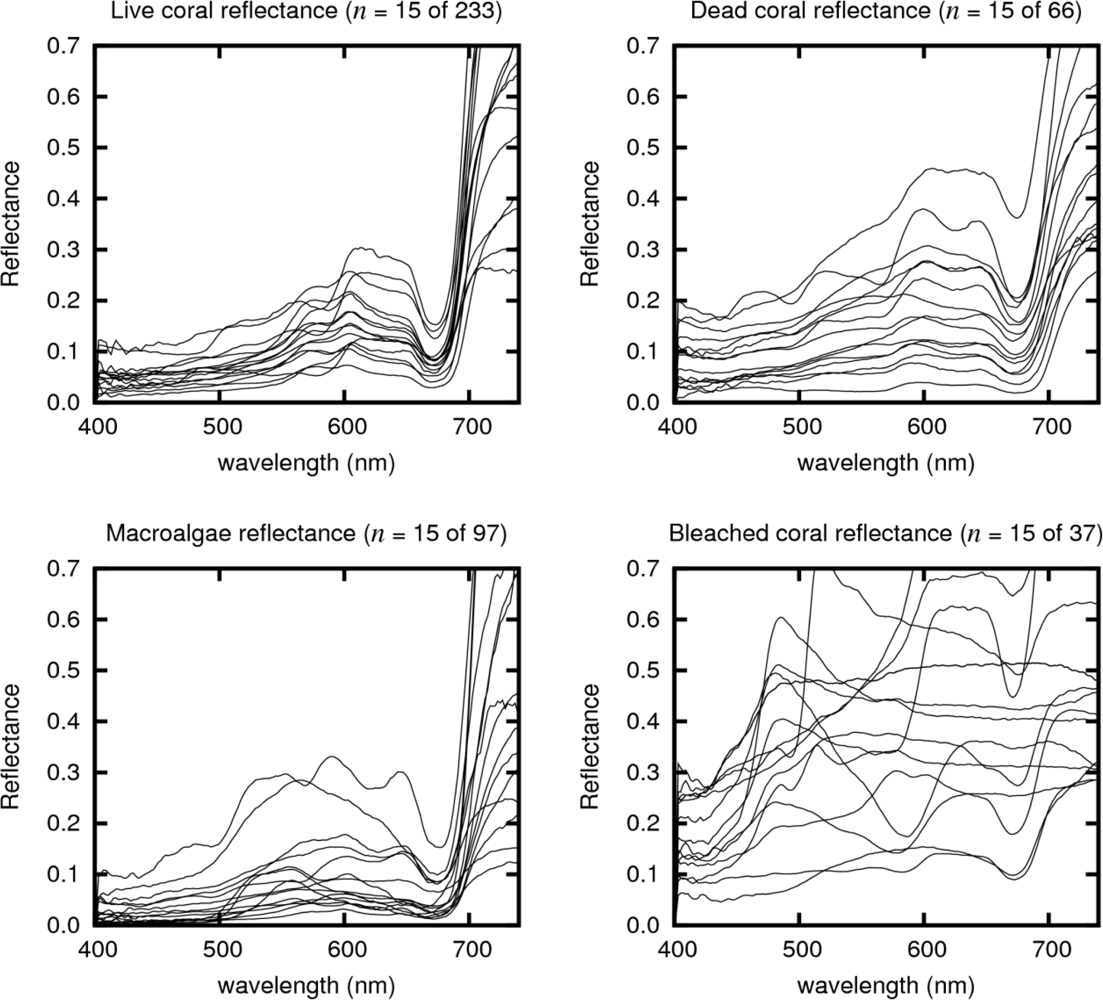
| Live Coral 100% cover | Each class is represented by 200 randomly generated diffuse spectral reflectance profiles constructed as a proportional linear mix between two random in situ reflectance spectra drawn from the field collected spectral library (Table 3, Figure 4). Linear spectral mixing at the bottom of the water column was therefore assumed [24]. The figure of 200 spectra per class was determined experimentally to ensure the variation in the in situ libraries was fully exploited while, for computational efficiency, excessive numbers of spectra were not propagated through the model (see Results and Discussion. | |
| Bleached Coral in Live Coral (proportion 1.0, 0.5, 0.2, 0.05) | ||
| Dead Coral in Live Coral (proportion 1.0, 0.5, 0.2, 0.05) | ||
| Macroalgae in Live Coral (proportion 1.0, 0.5, 0.2, 0.05) | ||
| Depth (6 Classes) | ||
| 0.5 m, 5 m, 20 m | Three image-uniform classes representing specific absolute depths of 0.5 m, 5 m and 20 m respectively. | |
| Shallow (0.5–2 m) | Three image-variable classes each of which models a remotely sensed image in which variation in depth is present. Shallow contains the two depths 0.5 m, 2 m; Shallow-Mid contains, 0.5 m, 2 m and 5 m; | |
| Shallow-Mid (0.5–5m) | ||
| Shallow-Deep (0.5–20m) | Shallow-Deep contains those three plus 10 m and 20 m. For example, the structure of the Shallow-Deep class implies that one of every five image pixels on the reef would be at 20 m. | |
| IOPs (5 Classes) | ||
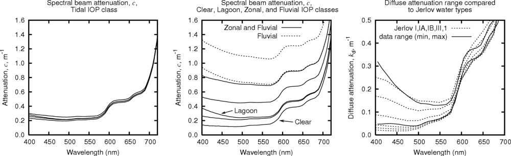
| Clear | An image-uniform class represented by a single IOP dataset from a fore reef drop-off site with strong tidal flushing (Figure 5) | |
| Lagoon | An image-uniform class represented by a single IOP dataset from a lagoonal station (Figure 5). | |
| Tidal | Image-variable class containing four datasets from a fore-reef location collected at two-hour intervals in a tidal cycle (Figure 5). | |
| Zonal | Image-variable class containing five IOP datasets from a mixture of lagoonal and fore-reef sites (Figure 5). | |
| Fluvial | Image-variable class with the same IOP datasets as Zonal plus two acquired at 0.6 km and 1 km offshore from a river outfall that passes through dense mangroves (Figure 5). | |
| Sun Elevation (2 Classes) | ||
| SH (zenith angle 15°) | Two image-uniform sky radiance distributions based on field data acquisitions of total and diffuse shaded downwelling irradiance collected in the marine tropics at two sun elevations. The directional sky radiance distribution was modelled as the sum of the direct sun radiance (total minus diffuse) and the diffuse irradiance directionally weighted by a clear sky radiance model [25]. | |
| SL (zenith angle 45°) | ||
| Wind Speed (2 Classes) | ||
| W2 (2 ms−1) | Two image-uniform water surface classes based on the approximate minimum and maximum daily wind speed averages taken over a one month period in Palau, April 2006 (this month coincides with a field study not reported here). These wind speeds are also similar to the range cited in previous remote sensing field studies, e.g., 2 ms−1 [9], ∼5 ms−1, [12]. The sea surface state is incorporated into the radiative transfer model by a statistical derivation of the directional light reflection and transfer with a relative sun and wind azimuth angle of 45°, modelled according to Cox and Munk wave slope statistics [26,27]. | |
| W8 (8 ms−1) | ||
| Sensor SNR (3 Classes) | ||
| 200:1 | Three SNR values defined as the ratio of the standard deviation of a normally distributed noise term to the signal level in each band [28]. Values were chosen to be representative of those cited for existing airborne remote sensing instruments (e.g., 480:1 and peak 790:1 for CASI and CASI-2, and 500:1 to 1000:1 for HyMap [29], www.itres.com). SNR classes implicitly embody within-image variance as they are a source of spectral variation on a pixel-by-pixel basis. | |
| 400:1 | ||
| 800:1 | ||
| Category | Total Spectra | Genera | Number of Spectra |
|---|---|---|---|
| Live Coral | 233 | Acropora | 87 |
| Porites | 45 | ||
| Montipora | 17 | ||
| Pocillopora | 12 | ||
| Favites | 7 | ||
| Millepora | 6 | ||
| Others (< 5 each) | 59 | ||
| Bleached Coral | 37 | Acropora | 32 |
| Others | 5 | ||
| Dead Coral/Turf Algae | 66 | N/A | |
| Macroalgae | 97 | Halimeda | 12 |
| Lobophora | 11 | ||
| Padina | 10 | ||
| Sargassum | 9 | ||
| Laurencia | 8 | ||
| Chlorodesmus | 7 | ||
| Dictyota | 6 | ||
| Caulerpa | 5 | ||
| Others (<5 each) | 29 | ||
| Sun Elevation and Wind Speed |
|---|
|
| Sensor SNR |
|
| Variation in Depth and Absolute Depth |
|
| Variation in IOP Values and Absolute IOP Value |
|
| Benthic Type vs. Pure Live Coral. | Mixture Proportion | Solar Zenith | Wind Speed | Depth Class | n | % of Sensor Limited Scenarios (Δτ̄ > 5%) | |
|---|---|---|---|---|---|---|---|
| % | degrees | ms−1 | 400:1 vs. 200:1 | 800:1 vs. 400:1 | |||
| Bleached Coral | any | any | any | any | 480 | 1 | 0 |
| Dead Coral | 5% | any | any | any | 120 | 0 | 0 |
| 20% | 45° | 2 | S | 15 | 73 | 33 | |
| M | 15 | 53 | 0 | ||||
| 8 | any | 30 | 16 | 0 | |||
| 15° | any | any | 60 | 2 | 3 | ||
| 50% | 45° | 2 | S | 15 | 73 | 53 | |
| M | 15 | 100 | 0 | ||||
| 8 | any | 30 | 37 | 33 | |||
| 15° | any | any | 60 | 17 | 13 | ||
| 100% | 45° | 2 | S | 15 | 53 | 67 | |
| M | 15 | 67 | 13 | ||||
| 8 | any | 30 | 43 | 17 | |||
| 15° | any | any | 60 | 17 | 13 | ||
| Macroalgae | 5% | any | any | any | 120 | 0 | 0 |
| 20% | any | any | any | 120 | 0 | 0 | |
| 50% | 45° | 2 | S | 15 | 67 | 33 | |
| M | 15 | 100 | 0 | ||||
| 8 | any | 30 | 20 | 10 | |||
| 15° | any | any | 60 | 13 | 3 | ||
| 100% | 45° | 2 | S | 15 | 53 | 60 | |
| M | 15 | 100 | 0 | ||||
| 8 | any | 30 | 30 | 17 | |||
| 15° | any | any | 60 | 13 | 10 | ||
| (1) Detecting proportions less than 100% of any benthic type. |
| (2) Water depth > 5m. |
| (3) Fluvial variation in IOPs when detecting bleaching. |
| (4) High sun elevation (zenith angle 15°vs. 45°). |
| (5) Water depth > 0.5 m when detecting bleaching (less important for dead coral or macroalgae). |
| (6) Sensor SNR, wind speed and other IOP variations are overall not very significant factors. |
Share and Cite
Hedley, J.D.; Roelfsema, C.M.; Phinn, S.R.; Mumby, P.J. Environmental and Sensor Limitations in Optical Remote Sensing of Coral Reefs: Implications for Monitoring and Sensor Design. Remote Sens. 2012, 4, 271-302. https://doi.org/10.3390/rs4010271
Hedley JD, Roelfsema CM, Phinn SR, Mumby PJ. Environmental and Sensor Limitations in Optical Remote Sensing of Coral Reefs: Implications for Monitoring and Sensor Design. Remote Sensing. 2012; 4(1):271-302. https://doi.org/10.3390/rs4010271
Chicago/Turabian StyleHedley, John D., Chris M. Roelfsema, Stuart R. Phinn, and Peter J. Mumby. 2012. "Environmental and Sensor Limitations in Optical Remote Sensing of Coral Reefs: Implications for Monitoring and Sensor Design" Remote Sensing 4, no. 1: 271-302. https://doi.org/10.3390/rs4010271