A Data Mining Approach for Sharpening Thermal Satellite Imagery over Land


Hydrology and Remote Sensing Laboratory, Agricultural Research Service, US Department of Agriculture, Beltsville, MD 20705, USA
*
Author to whom correspondence should be addressed.
Remote Sens. 2012, 4(11), 3287-3319; https://doi.org/10.3390/rs4113287
Submission received: 29 August 2012
/
Revised: 22 October 2012
/
Accepted: 22 October 2012
/
Published: 26 October 2012
(This article belongs to the Special Issue Thermal Remote Sensing Applications: Present Status and Future Possibilities)
Abstract
:Thermal infrared (TIR) imagery is normally acquired at coarser pixel resolution than that of shortwave sensors on the same satellite platform and often the TIR resolution is not suitable for monitoring crop conditions of individual fields or the impacts of land cover changes that are at significantly finer spatial scales. Consequently, thermal sharpening techniques have been developed to sharpen TIR imagery to shortwave band pixel resolutions, which are often fine enough for field-scale applications. A classic thermal sharpening technique, TsHARP, uses a relationship between land surface temperature (LST) and Normalized Difference Vegetation Index (NDVI) developed empirically at the TIR pixel resolution and applied at the NDVI pixel resolution. However, recent studies show that unique relationships between temperature and NDVI may only exist for a limited class of landscapes, with mostly green vegetation and homogeneous air and soil conditions. To extend application of thermal sharpening to more complex conditions, a new data mining sharpener (DMS) technique is developed. The DMS approach builds regression trees between TIR band brightness temperatures and shortwave spectral reflectances based on intrinsic sample characteristics. A comparison of sharpening techniques applied over a rainfed agricultural area in central Iowa, an irrigated agricultural region in the Texas High Plains, and a heterogeneous naturally vegetated landscape in Alaska indicates that the DMS outperformed TsHARP in all cases. The artificial box-like patterns in LST generated by the TsHARP approach are greatly reduced using the DMS scheme, especially for areas containing irrigated crops, water bodies, thin clouds or terrain. While the DMS technique can provide fine resolution TIR imagery, there are limits to the sharpening ratios that can be reasonably implemented. Consequently, sharpening techniques cannot replace actual thermal band imagery at fine resolutions or missions that provide high quality thermal band imagery at high temporal and spatial resolution critical for many agricultural, land use and water resource management applications.
The US Department of Agriculture (USDA) prohibits discrimination in all its programs and activities on the basis of race, color, national origin, age, disability, and where applicable, sex, marital status, familial status, parental status, religion, sexual orientation, genetic information, political beliefs, reprisal, or because all or part of an individual’s income is derived from any public assistance program. (Not all prohibited bases apply to all programs.) Persons with disabilities who require alternative means for communication of program information (Braille, large print, audiotape, etc.) should contact USDA’s TARGET Center at (202) 720-2600 (voice and TDD). To file a complaint of discrimination, write to USDA, Director, Office of Civil Rights, 1400 Independence Avenue, S.W., Washington, DC, USA, 20250-9410, or call (800) 795-3272 (voice) or (202) 720-6382 (TDD). USDA is an equal opportunity provider and employer.
1. Introduction
Thermal infrared (TIR) remote sensing provides spatially distributed estimates of land-surface temperature (LST) that can be used for detecting wild fires [1,2], mapping land surface energy fluxes and evapotranspiration [3–10], monitoring urban heat fluxes [11–15] and detecting drought [7,8,16]. For many of these applications, TIR data are required at relatively fine resolution. However, thermal band imagery is normally acquired at a coarser pixel resolution than that of shortwave sensors on the same satellite platform. Table 1 lists spatial resolutions of shortwave and TIR bands for several medium resolution sensors including the Thematic Mapper (TM; Landsat 5), the Enhanced Thematic Mapper Plus (ETM+; Landsat 7), the Thermal Infrared Sensor (TIRS) and Operational Land Imager (OLI) package to be flown on the Landsat Data Continuity Mission (LDCM), as well as the Advanced Spaceborne Thermal Emission and Reflection Radiometer (ASTER). The spatial resolutions of shortwave spectral band imagery for these medium resolution sensors vary from 15 to 30 m, while TIR resolutions range from 60 to 120 m. Though the 60–120 m pixel resolution may meet requirements for applications in some regions, a finer TIR pixel resolution is desired for many heterogeneous areas, particularly agricultural regions containing small (∼1 ha) fields [3,9,17,18].
To improve spatial resolution in LST retrievals, several techniques have been developed to sharpen thermal band imagery using shortwave band data. These sharpening techniques are often referred to as downscaling or disaggregation techniques in previous publications. The basic assumption of most thermal sharpening approaches is that land surface temperature (LST) has a unique relationship to shortwave band signals across a given imaging scene. Relationships between LST and spectral signals within a scene are determined empirically at the coarse (thermal band) pixel resolution and then applied to the fine (shortwave band) pixel resolution to produce sharpened thermal band imagery. A classic sharpening technique, TsHARP, sharpens thermal data using an inverse relationship developed between the surface temperature and the Normalized Difference Vegetation Index (NDVI) [3,17]. Agam et al.[17] evaluated four different LST-NDVI functions and found fractional vegetation cover (fc) computed from NDVI yielded the smallest prediction errors for LST.
TsHARP assumes that the LST-fc (or LST-NDVI) relationship is unique for different land cover types at different spatial resolutions and locations. This assumption is reasonable for a uniformly (homogeneous) vegetated area and worked well in rainfed agricultural areas [17,19]. However, several studies have demonstrated that the LST-NDVI relationship is not well-defined over many complex heterogeneous landscapes [13,20–25]. To address this issue, Inamdar and French [20,21] used emissivity data to sharpen GOES land surface temperature over the US Southwest. Merlin et al.[22] developed separate LST-NDVI relationships for photosynthetically and non-photosynthetically active vegetation cover to sharpen imagery over an irrigated crop land in Mexico. Dominguez et al.[13] found that the LST-NDVI relationship was ill-defined over an urban area in Puerto Rico, and included albedo as an independent variable in their High-resolution Urban Thermal Sharpener (HUTS), which yielded smaller Mean Absolute Error (MAE) and higher correlation coefficient compared to TsHARP [13]. Jeganathan et al.[23] investigated the TsHARP approach over a mixed agricultural landscape in India and suggested the approach could be applied locally within relatively homogeneous sub-regions, but not on a regional basis. Chen et al.[24] found the relationship between LST and vegetation index depends on image spatial extent.
While these refinements to the original TsHARP approach share a similar conceptual framework, namely developing relationships between LST and spectral signals or derived biophysical parameters at coarse pixel resolution and then applying to spectral imagery at fine pixel resolution, they differ in the selection of predictor variables used in the sharpening approach. Sharpening techniques dependent on higher order products as input (e.g., albedo, land cover type and emissivity) are less easily applied in an automated operational data production system, and different inputs may be important over different landscapes. The choice of an optimal prediction model (e.g., linear vs. non-linear) may also vary from location to location, so more flexibility in model construction is needed for routine, global application.
The objective of this paper is to establish a robust sharpening technique that can be applied operationally to landscapes and conditions at different spatial resolutions, and does not need higher order data products as input. A data-mining sharpening method (DMS) is described that relates TIR temperature directly to a suite of shortwave spectral reflectances using a regression tree approach. In this method, there is no pre-selection of which shortwave band combinations are important for a particular landscape; rather, this is determined adaptively by the DMS. The method is designed to utilize the full complement of TIR and shortwave data collected by a given satellite platform.
The performance of the DMS and TsHARP approaches is evaluated at three sites that represent very different vegetation and moisture conditions. These include a rainfed corn and soybean production region in central Iowa, an irrigated agricultural region growing primarily wheat, cotton, corn and sorghum in the Texas High Plains, and a complex heterogeneous naturally vegetated landscape in Alaska containing a variety of forests, open grass and shrublands, and open water surfaces. Landsat TM, ETM+ and airborne surface and top-of-atmosphere (TOA) brightness temperatures are used in evaluating the sharpening approaches. Results from the DMS are compared to TsHARP and to the uniTR method, which assumes no subpixel variation in LST (i.e., no sharpening).
2. Approach
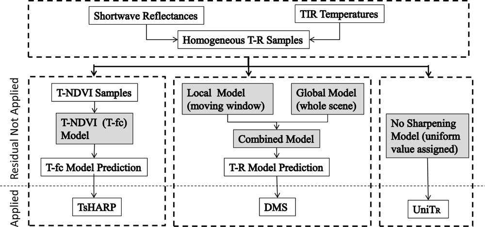
DMS uses reflectances from shortwave spectral bands as independent variables. Reflectance (either top-of-atmosphere or surface) data from shortwave spectral bands are aggregated to match the coarser TIR band pixel resolution. Then, high-quality land surface temperature (T) and reflectance (R) data points selected from the imagery (referred to as “samples”) are used to build the T-R relationship using a regression tree method [26,27]. In the DMS, the T-R regression trees (also referred to as the T-R model) built from coarse resolution samples are then applied to fine resolution shortwave spectral reflectance to predict TIR temperature at the finer pixel resolution. Finally, the predictions of temperature from the T-R regression tree at fine resolution are aggregated to TIR band resolution and the differences (residuals) at coarse resolution are uniformly redistributed across the fine-scale T values within each coarse pixel to ensure that the sharpened map will reaggregate to the unsharpened values. Although this sharpening procedure is similar in many aspects to other techniques, the selected predictor variables and the T-R regression tree method are unique. Several factors that must be considered in the DMS thermal sharpening process are discussed below.
2.1. Data Mining Model for LST and Shortwave Spectral Reflectance
The original TsHARP approach assumed a specific T-NDVI functional relationship (linear or non-linear) and used this to sharpen the TIR image to the finer NDVI resolution. While this has the advantage of simplicity, as noted above the T-NDVI relationship is not unique for a variety of land cover conditions and hence robust sharpening requires additional information such as land cover type, fraction of green vegetation, emissivity, or surface albedo [13,21,22]. To efficiently handle the large number of input variables that may influence LST distributions across different landscapes, we have adopted a data mining approach, which searches for patterns among data samples used for training. There are several advantages to this approach. First, data mining approaches do not rely on any pre-defined relationship between the variables. The data-driven method itself determines scene-relevant relationships based on the sample features extracted from the scene, allowing ready application over different locations and conditions. Second, temperature and spectral reflectance samples are extracted from all regions across the scene, providing well distributed samples (for training the data mining model. Third, the sample size is large, which ensures the model predictions can be evaluated using standard statistical measures. In this paper, the cubist regression tree method [26,27] is applied to train the temperature and spectral reflectance relationships.
Reflectances from the spectral bands contain information about surface type and albedo that may not be provided by NDVI alone. The regression tree method generates rule-based multivariate regressions from the T-R samples, and these rules can separate different trends found among the T-R data within the scene. For each rule, the multivariate regression is assumed to be linear. A linear relationship between surface reflectance and temperature is supported by observations from earlier studies [28]. While a higher order polynomial function may be better able to capture the variations of temperature, it has a risk of over-fitting and may be too sensitive to noise in the samples [17]. As the DMS uses reflectances as independent variables directly, it eliminates extra processing including mapping land cover, and computing albedo and fractional vegetation cover. In addition, because the DMS does not rely on pre-assumed relationships, it is easy to include additional independent variables (e.g., emissivity, soil moisture, hill shade relief, etc.) in the processing where identified as necessary [29].
2.2. Homogeneous Samples and Weighting Function
The original TsHARP approach assumes the T-NDVI relationship is universal at different spatial resolutions. If this is true, T-NDVI relationships built from coarse resolution images can be applied at fine resolution. However, as the aggregation procedure for temperature is non-linear, while aggregation for reflectance is linear, the T-R and T-NDVI relationships for the mixed pixels may indeed vary with spatial resolution. Nevertheless, the T-R relation will be applicable if the coarse resolution pixel is homogeneous. Kustas et al.[3] suggested selecting coarse resolution samples with the lowest 25% coefficient of variation in NDVI to develop the T-R sharpening relationships. This practical strategy not only screens out outliers but also preserves homogeneous pixels for the training process. In this paper, a coarse resolution sample is defined as “homogeneous” if sub-pixel reflectances at the fine (spectral band) resolution are similar, i.e., the subpixel variation in coarse resolution pixel is close to zero. Note that the fine resolution pixel does not necessarily have to be “pure” by this definition. In the DMS, homogeneous samples used to train the regression trees are selected on the basis of the averaged coefficient of variation of the sub-pixel reflectances, defined as:
where subscript i represents the spectral band, n is the total number of spectral bands, μ and σ are the mean and the standard deviation of the fine resolution reflectances within the coarse resolution pixel, respectively. Clearly, the smaller the cv value, the purer the sample, but in practice a purely homogenous pixel (cv = 0) is unlikely. Consequently, the criterion was relaxed and a threshold for a useable sample was defined as cv < 0.20 (or 20%). In the case studies presented here, this threshold (cv < 0.20) resulted in 80–90% of the pixels in the sampling window being classified as useable samples. These useable pure samples were then weighted inversely by cv in the multi-variant regression, giving purer samples more weight.
2.3. Global and Local Regression Models
The T-R relationship may vary across a given scene due to differences in factors controlling LST (e.g., soil moisture, vegetation cover, or air temperature). In these situations, a regression model built from samples selected locally (e.g., close to the coarse TIR pixel that is being sharpened) will typically work better than a global regression model built from samples selected across the whole scene [23–25]. A local model can be implemented using a moving window, where local regressions are determined within some predefined window and applied to coarse pixels within that window. To avoid boundary effects, where discontinuous changes in the regression model between windows may lead to artificial box-like discontinuities in the sharpened LST imagery, an overlapping moving window approach was adopted. The central window of the prediction area (the area of regression application) was defined according to the complexity and soil moisture conditions in the area. The sampling area (the area from which training samples were extracted) is an extension of the prediction area, with approximately double the size. This ensures that adjacent moving (prediction) windows share some common samples, which reduces the window boundary effect. The default window sizes for prediction and sampling area were defined as 50 by 50 and 72 by 72 respectively. For the irrigated case study site (Section 3.2), the window sizes were reduced to 10 and 14 for the prediction and sampling areas to account for the complex irrigation patterns. A smaller window size may be able to capture local variation of T-R relationship but will also reduce the number of samples available for training. A T-R relationship established based on a limited number of samples may not reliable. In practice, the smaller window size demands more computing time for the entire area. Thus in our tests, the prediction windows size was set between 10 (very complex) to 50 (relative homogeneous). The number of rules which determine the number of regression tree nodes in the cubist algorithm was constrained to be less than five in the application of the local model, but it was unconstrained in the global model.
Although a local model generally performs better than a global model [23–25], the prediction accuracy may be low if T-R samples are not well distributed over the full range of expected T and R in the sampling area. In this case the regression tree predictions must extrapolate significantly beyond the training data, especially for small outlier features that are not well-represented in the homogeneous training data (e.g., small irrigated fields that are not resolved at the TIR pixel scale). In these cases, the global model may outperform the local model since the global samples are likely to include a wider range of conditions. In the DMS, both the global and the overlapping moving window approaches are implemented over each scene and the accuracy is evaluated for each coarse resolution TIR pixel by examining the residuals. The final (combined) model prediction (p) is computed using a weighted linear combination of local and global model results as:
where pi represents the prediction from the local or global model, wic is the weight at coarse resolution, and the subscript c represents coarse resolution. The prediction (local or global) with the smaller residual at a given coarse resolution pixel represents a better prediction and thus is weighted higher using the reversed squared residual as:
where ric is the residual for the local and global model prediction at coarse resolution.
2.4. Residual Analysis
Ideally, if the underlying model prediction is accurate, there should be no bias between the original TIR image and the sharpened image aggregated to the coarse native TIR resolution. In general, however, models are imperfect and the available spectral bands do not contain all the information necessary to reconstruct LST at finer resolutions. To enforce energy conservation within the sharpening process (e.g., near-perfect aggregation to the original TIR image), residuals between predicted and observed LST fields at the coarse resolution are redistributed over the sharpened LST maps. This application of residuals in the sharpened imagery can sometimes cause artificial box-like features that are visible at the native LST resolution if there are significant inaccuracies in the sharpening model. To reduce the appearance of these box-like features, the coarse resolution residual fields can be spatially smoothed using a Gaussian filter prior to reintroduction into the sharpened map [6]. However, Merlin et al.[22] argue that more accurate models, that more fully capture signals of the various factors controlling LST variability over the scene, will necessarily reduce the magnitude of these residuals. Therefore, residual analysis becomes an effective tool for evaluating model performance and is used in the DMS to weight global and local model predictions at the coarse resolution pixel level.
2.5. Comparative Sharpening Techniques
The DMS TIR-band sharpening approach developed in this paper is compared to two additional techniques. The uniTR approach uniformly distributes the coarse resolution LST values over the finer pixel resolution sub-pixels; in other words, the LST field is not actually sharpened. The uniTR method represents the simplest possible disaggregation strategy (using no additional input variables), and therefore is used as a relative metric for evaluating the performance of the other sharpening approaches.
TsHARP was also applied to the test scenes, using the formulation from Agam et al.[17] based on the vegetation cover fraction (fc) derived from NDVI. TsHARP represents a global modeling approach, where the T-fc sharpening regression is built from homogeneous samples selected over the whole scene (the same set used for the global DMS model).
Figure 1 illustrates the data processing flow chart for this paper. Data from Landsat TM, ETM+ and from an airborne imaging system were used in the tests. The TIR images were aggregated from their native resolution to a set of coarser resolutions, and then sharpened back to a reference T resolution. Two simple statistical criteria were used to evaluate model performance; mean absolute error (MAE) and the coefficient of determination (r2) between predicted and reference LST.
3. Test Sites and Data Preparation
The three sharpening approaches (DMS, UniTR and TsHARP) were applied to TIR and shortwave imagery collected over three different areas representing rainfed and irrigated agricultural areas, and a heterogeneous naturally vegetated landscape. The test sites and image characteristics are described below.
3.1. Rainfed Agricultural Site
A relatively homogeneous rainfed agricultural site in central Iowa was selected for analysis, with nearly 95% of the land area in either corn or soybean production, and the remaining 5% constituting small forest stands, grasses, water, bare soil and impervious surfaces (e.g., buildings and roads). The selected Landsat scene listed in Table 2 (WRS-2 path 26 and row 31, with central location (41.8°N, 93.0°W)) covers the Soil Moisture-Atmosphere Coupling Experiment (SMACEX), which was conducted in central Iowa during 2002 [5]. Three Landsat 7 ETM+ images acquired on 14 May, 1 July and 22 November 2002 were obtained for evaluating the sharpening procedures, representing conditions at the start, peak and end of the growing season. Scene-average NDVI for the three dates varied from 0.24 to 0.64, while surface temperature varied from 5.5 to 36.9 °C with scene-based standard deviations of 1.7 to 4.0 °C.
Multi-spectral airborne imagery was also collected over the Iowa campaign site during SMACEX [19]. Airborne TIR images collected on 1 July 2002 at 6 m pixel resolution using an Inframetric 760 scanner were used to validate results from the different sharpening approaches.
3.2. Irrigated Agricultural Site
The sharpening approaches were also evaluated over an irrigated agricultural site, where fine-scale LST variability is often more strongly correlated with surface moisture conditions than with vegetation cover amount. In such landscapes, an NDVI-only based sharpening approach, such as TsHARP will miss a significant component of LST variability, for example, missing low-LST sub-pixel features associated with fields that received pre-emergence irrigation (no NDVI signal). This leads to large residuals in the TsHARP approach, causing box-like features to appear in the sharpened LST fields [18]. The sharpening approaches were applied to the Landsat TM scene in Table 2 (WRS-2 path 31 and row 36, central location (34.61°N, 102.92°W)) acquired over the northern part of the Texas and New Mexico state boundary lines on 22 September 2002. This scene was used in a previous case study [18] to test TsHARP over irrigated agricultural fields in the Texas High Plains. The scene includes both irrigated and rainfed agriculture (primarily cotton, wheat, corn and sorghum). September is a relatively dry month in this region and many of the fields containing near-mature cotton and emerging winter wheat were receiving irrigation.
3.3. Complex Terrain Site
Thermal sharpening is particularly challenging over heterogeneous sites where there is significant sub-pixel variability in LST caused by multiple uncorrelated factors such as shading and elevation. Such a site was selected for evaluating sharpening approaches over a heterogeneous naturally vegetated area in Alaska with varying topography included within Landsat TM WRS-2 path 73 and row 12 centered at 68.3°N, 150°W, using an image acquired on 5 July 2009 (Table 2). The northeast portion of the scene has flat terrain and was clear on the imaging date, while the southwest part of the scene covers rugged/complex terrain and was partially cloud covered. Land cover contained in this complex scene was a mixture of deciduous and coniferous forests, tundra and open water surfaces. This scene exhibited a weak positive relationship between LST and NDVI, typical of natural and agro-ecosystems that are energy limited and/or affected by elevation/terrain, and in contrast with the negative relationship found when moisture is the growth limiting factor [30]. Unlike the agricultural scenes discussed above, topography may play a role in controlling surface temperature in this scene.
3.4. Data Preparation
Both Landsat TM and ETM+ data were calibrated to top of atmosphere (TOA) reflectance and brightness temperature using Landsat Ecosystem Disturbance Adaptive Processing System (LEDAPS) [31]. In practice, the DMS sharpening process could either be applied to atmospherically corrected surface reflectance and temperature images, or simply to the TOA (uncorrected) reflectances and brightness temperatures, depending on operational constraints. In this study, the TOA reflectance and brightness temperature were used in most tests, except for the rainfed agricultural site on 1 July, where surface products from a previous study [32] were used. The thermal band airborne imagery from SMEX02 was also calibrated and atmospherically corrected to surface temperature, and was used in a previous sharpening study [17].
Reflectances were aggregated from fine resolution to coarse resolution using simple areal averaging. To aggregate TIR fields, LST was first converted to radiance according to the Stefan-Boltzmann law:
where ε is the emissivity and σ is the Stefan-Boltzmann constant, T is the LST in K. As accurate emissivities at the fine resolution are typically not available, we simply assume the emissivities of adjacent fine resolution pixels are similar, thus the aggregated temperature was computed as
where n represents total number of fine resolution pixels in the coarse resolution cell. Note that this may not be a reasonable approximation under conditions of strongly heterogeneous terrain [33]. Following the Stefan-Boltzmann law, the 4th power of temperature was used for pixel aggregation, disaggregation and residual temperature redistribution. The sharpened radiance images were converted to temperature in the final step.
In this study, several sharpening scenarios were simulated covering a wide range of thermal-toshortwave resolution ratio (sharpening ratio). For ETM+ scenes, the spectral band images were aggregated to 60 m pixel resolution to match the native TIR band resolution. The TIR image was then aggregated to coarser spatial resolutions of 120, 240, 480 and 960 m pixel resolution then sharpened to 60 m resolution, using the original ETM+ TIR image at 60 m spatial resolution as a reference to validate sharpening results (Table 2). These tests cover a wide range of sharpening ratios from 2 to 16. For most satellite missions, the thermal-to-shortwave resolution ratio for the same satellite platform varies from 2 to 6 as shown in Table 1.
For Landsat TM scenes, Landsat TM spectral reflectances were aggregated to 120 m to match the native resolution of the TIR band, and the TIR band image was aggregated to spatial resolutions of 240, 480 and 960 m. These images were sharpened to 120 m, and compared to the original LST image at 120 m resolution (Table 2). The TM tests therefore evaluate sharpening ratios from 2 to 8.
For the irrigated site (Landsat WRS-2 path 31 and row 36), the original Landsat ETM+ TIR image at 60 m spatial resolution was aggregated to coarser spatial resolutions of 120, 240, 960 m pixel resolution. The simulated TIR image at 960 m resolution was then sharpened to 60, 120, 240 m resolution and validated using the ETM+ TIR image at corresponding spatial resolution as a reference.
Finally, fine-resolution (6 m) airborne TIR images acquired during the SMACEX’02 campaign (over the rainfed agricultural site) on 1 July 2002 were used to evaluate the sharpening to 30 m, as it would be applied in practice to Landsat TM, ETM+ and to OLI/TIRS data from LDCM. The airborne TIR band image was geo-referenced, mosaicked and corrected for atmospheric and emissivity effects [17]. The corrected 6-m TIR image was aggregated via Equation 3 to 30 m resolution for validating sharpening techniques at the scale of operational application for Landsat TM and LDCM (120 m to 30 m). In the study, we assume TIR image and shortwave band images have been cross-registered with sufficient accuracy from Landsat missions [34].
4. Results and Analysis
The DMS involves several components that differ from the standard TsHARP technique; hence, the DMS–TsHARP comparisons were evaluated in sequential steps for each additional DMS refinement, as applied to the rainfed agricultural site. The full DMS approach is then compared with TsHARP and uniTR results over each of the three test sites in the latter subsections.
4.1. DMS Component Analysis
As a first step, the relative performance of the underlying T-fc relationships used in the TsHARP formulation, namely fc as the independent variable in a linear regression with T, was evaluated vs. using all shortwave band reflectances in a regression tree (DMS). Next the impact of using a global vs. local model to construct the reflectance-based regression tree in the DMS was examined. Lastly, the impact of adding the residuals back into the sharpened LST fields from both approaches was investigated.
4.1.1. Reflectance Suite vs. fc as Independent Variables
The DMS approach uses all spectral band reflectances as independent variables, while the TsHARP approach uses only fc derived from NDVI as the independent variable in a linear regression model. To compare sharpened results from these approaches, the same homogeneous samples extracted from the whole image (global) to train T-fc and T-R functions (i.e., the global T-R model was applied) were used for three dates over the rainfed agricultural site. In these comparative tests, ETM+ TIR data were sharpened from 120, 240, 480 and 960 m down to 60 m resolution. Here we test the capacity of the underlying relationships (T-fc and T-R) to capture LST variability prior to reintroduction of residuals, noting that better functions will necessarily yield smaller residuals.
Table 3 lists the MAE and r2 computed between model predictions and reference temperatures at 60 m resolution from the resulting 12 tests (4 sharpening ratios on 3 dates). In all tests, the global T-R model predictions yield smaller MAE values compared the T-fc model. The magnitude of MAE from the global T-R model depends on sharpening ratio, with smaller sharpening ratios yielding smaller errors. The T-fc model yields similar MAE values across different sharpening ratios, which implies that a unique T-fc relationship exists for each date across different spatial resolutions. For the three testing dates, MAE from global T-R model are smaller than those from T-fc by 0.40–0.69, 0.38–0.49 and 0.45–0.59 °C (or K) for 14 May, 1 July and 22 November respectively.
In Table 3, r2 values from the global T-R model are higher (>0.64) than those from the T-fc model (<0.62) for all stages in the growing season. The most dramatic improvement comes from the scene late in the season, when the vegetation was predominantly senescent (22 November, NDVI = 0.24). In this case, r2 improved from 0.08 to >0.64 by using the T-R global model. However, the T-fc model still works reasonably well for much of the growing season as previous studies have found [17,22].
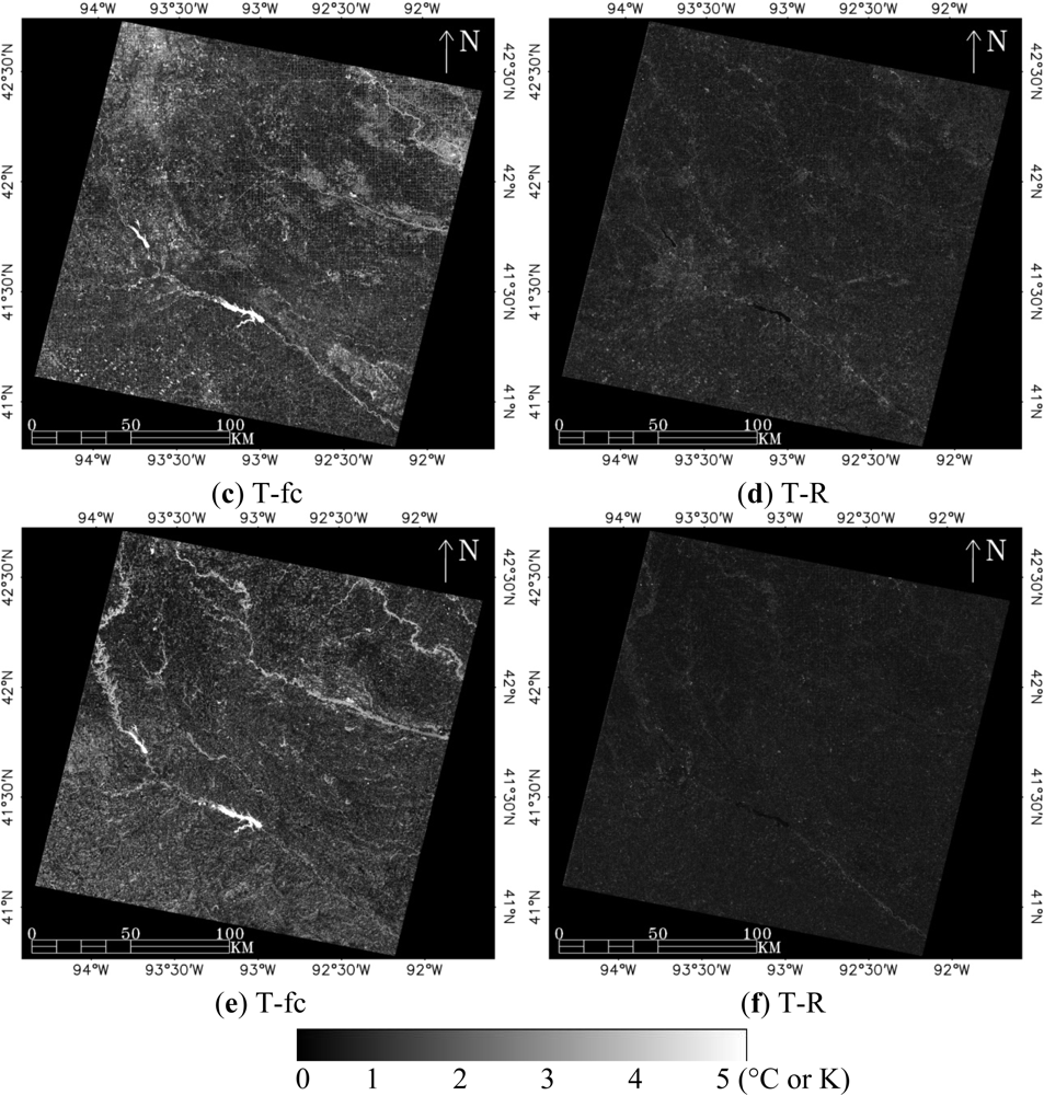
The absolute differences (absolute residuals) between model predictions and reference temperatures from the three test dates are shown in Figure 2. In the figure, darker colors indicate smaller differences and brighter colors show larger differences. Again, the same training datasets have been used for both the T-fc model and global T-R model. For the T-fc model, larger residuals are seen in the non-vegetated areas such as bare soils, rivers and urban areas. Temperature variations in these areas are therefore less well correlated with fc. As the global T-R model used all spectral reflectance bands, trained with a regression tree rather than a fixed relationship, different T-R patterns were detected and separated for different surface types. The predictions from the global T-R model show smaller residuals for both vegetated and non-vegetated surfaces.
4.1.2. Global and Local Regression Models and Combined Approach
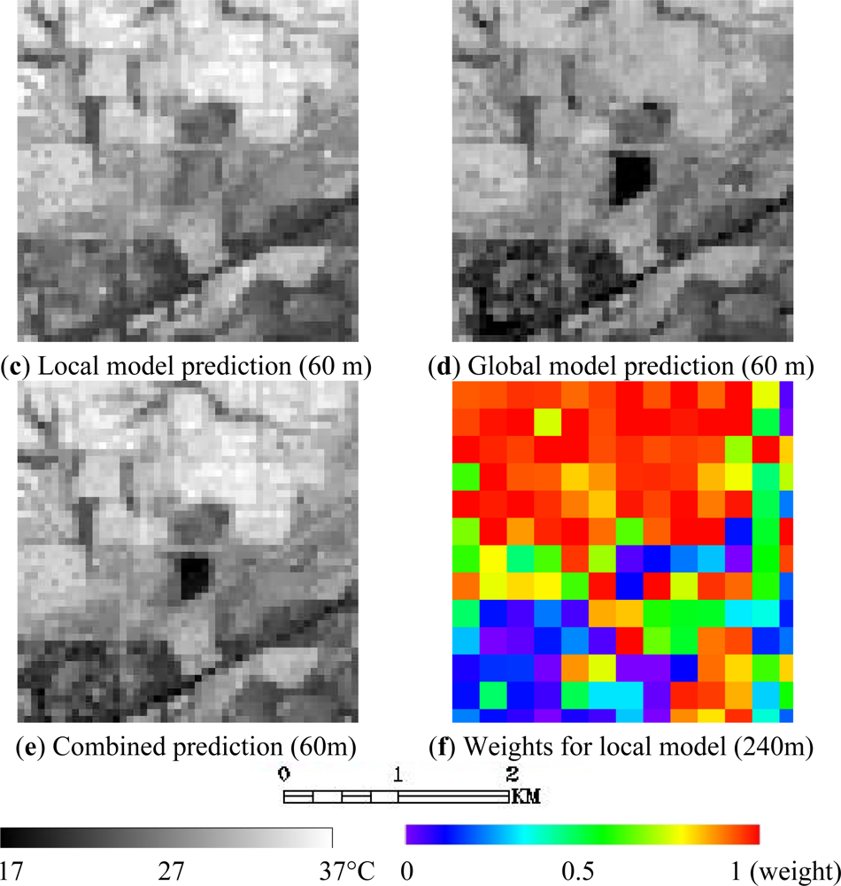
Table 3 also lists statistics comparing T-R results from the local modeling approach (selecting samples locally from an overlapped moving window). In all test cases, the MAE from the local T-R model was smaller than for the global T-R model by 0.32–0.45, 0.14–0.27 and 0.10–0.12 K for 14 May, 1 July and 22 November respectively. The coefficients of determination from the local model were higher than the global model, indicating overall better performance. However, in some cases where small outlier features were not well-represented in the moving window, the local model predictions were less accurate as demonstrated in Figure 3. In this figure, the circled object (presumably an agricultural field with high moisture conditions and low T) represents a small population of T-R samples that was not accurately predicted by the local model. In contrast, the global model was able to capture this population by using samples selected from the entire scene, although it did not perform as well as the local model in other parts of this sub-scene.
To generate an optimal combination of local and global modeling results, local and global regression model output were combined. First, the residuals from local and global models were computed at the TIR pixel resolution, and then the residuals from the two models were converted to weights for each TIR pixel. The model result with smaller residuals is normally a better prediction and thus weighted higher using Equation (3). The combined result is shown in Figure 3 along with the weight from the local model prediction. The local model outperformed the global model in general, with weighting values >0.5 as shown in Figure 3f. However, the global model worked better in the lower left part of the image. Comparing the reference temperature field (Figure 3(b)) with output from the combined model (Figure 3(f)) indicates that the combined model outperformed both the local and global models. MAEs reduced from 1.47 K (global model) and 1.11 K (local model) to 1.03 K for the combined model for the entire Landsat scene on 14 May.
4.1.3. Impact of Residuals
All thermal sharpening techniques redistribute the T residuals to ensure energy conservation in the sharpened imagery (i.e., ensure that the sharpened T map aggregates to the unsharpened or native resolution T values). Table 4 lists MAE values before and after redistributing residuals for the TsHARP and DMS approaches. Note that in Table 4, the combined T-R (global and local) model was used and thus the MAE is smaller than that obtained from the local or global model alone, listed in Table 3. Application of residuals reduces MAE with respect to reference fields for both TsHARP and DMS. TsHARP shows notable reduction in MAE after reintroduction of residuals, ranging from 0.32 °C (960 to 60 m on Nov. 22) to 1.57 °C (120 to 60 m on 15 May). In contrast, residual redistribution has a smaller improvement for DMS (0.05 to 0.35 °C) because the combined T-R model already accurately captured much of the extant variability in surface temperature.
Although the redistribution of residuals ensures conservation of energy and reduces MAE, it yields no new information about sub-pixel variation in thermal band imagery. The subpixel information only comes from sharpening model algorithm or relationship developed between T and the shortwave band data. Smaller MAE values from the underlying algorithm in the sharpening model, namely T-fc for TsHARP and T-R for DMS, are what determine the accuracy of the sharpening process. The utility of the TsHARP and DMS models in sharpening T is examined in the following three case studies.
The relative performance of different sharpening models, after redistributing residuals, is also reflected in coefficients of determination computed with respect to the reference temperature fields, as shown in Table 5 and using uniTR (no sharpening) as a basis for comparison. Even the non-sharpening uniTR approach shows very high correlation (r2 > 0.78) in first two rows, which implies the rainfed agricultural site is relatively homogeneous from 60m to 240 m pixel resolution. In all testing cases, the DMS approach shows the highest correlation in each group. The most significant difference in performance was found for the November 22 image, when there was little green or active vegetation present. The original r2 between the 960 m and 60 m resolution images was 0.45 (uniTR). The correlation for the TsHARP model before applying residuals was very weak (r2 = 0.08 in Table 3). After applying residuals, results for the TsHARP approach improved to 0.46. In contrast, r2 from the DMS model only increased from 0.71 to 0.77 after applying residuals. This indicates that the additional reflectance bands used in the DMS regression tree allowed more of the variability in surface temperature to be captured over this scene, which was mainly comprised of senescent vegetation.
4.2. Results from the Rainfed Agricultural Site
4.2.1. Landsat Simulations
Figure 4 illustrates the final sharpening results from the uniTR, TsHARP and DMS approaches for a subset area within the rainfed agricultural site. The top row shows the ETM+ reference temperature maps for 14 May, 1 July and 22 November at 60 m spatial resolution. The uniTR approach (second row) shows results at 240 m resolution (i.e., no sharpening). The TsHARP (third row) and DMS (fourth row) images have been sharpened from 240 to 60 m pixel resolution. The results from TsHARP and DMS show clear agricultural field boundaries and reasonable sub-pixel variations in temperature, particularly when compared to uniTR. The TsHARP approach yielded more accurate sharpening results on 14 May and 1 July than on 22 November, when the variation in T was not related to green vegetation cover. In all 3 scenes, box-like anomalies associated with water bodies and bare soil are visible in the TsHARP results, indicating these areas were not well-captured by the T-fc relationship and therefore had large residuals. The DMS outperformed TsHARP for all dates and areas, including vegetated and non-vegetated surfaces, as is demonstrated both visually (Figure 4) and statistically (Tables 4 and 5).
4.2.2. Airborne Imagery Simulations of Landsat Sharpening
To simulate sharpening of Landsat 5 and LDCM data from 120 to 30 m, the 6 m resolution airborne surface temperature image on 1 July 2002 acquired over the SMACEX’02 site was aggregated to 30 and 120 m resolution. The uniTR, TsHARP and DMS approaches were applied to sharpen the 120 m surface temperature field back to 30 m and then compared to the 30 m resolution reference temperature (Figure 5). Similar to the ETM+ results in Figure 4, both TsHARP and DMS recover sub-pixel information that is unresolved by the uniTR approach. However, the DMS model yields sharpened T with better accuracy for non-vegetated surfaces such as roads and rivers.
Another test of the sharpening techniques involved satellite and airborne observations acquired on 1 July 2002 over the SMACEX ’02 site. Landsat ETM+ TIR data (60 m resolution) were re-sampled to 30 m resolution using cubic convolution in the standard Landsat data product from US Geological Survey (USGS) Earth Resources Observation and Science (EROS) data center. The 30 m resolution ETM+ TIR data were aggregated to 120 m pixel resolution and sharpened to 30 m using the 3 approaches, with a subset window shown in Figure 6. Temperatures from the airborne measurement and the Landsat ETM+ subset have different mean values (39.5 °C vs. 37.5 °C) and standard deviations (5.7 °C and 3.3 °C), so a different data stretch color schema for the two data sources was applied in Figure 6. Nevertheless, the spatial patterns of surface temperature from both systems are comparable. In Figure 6, both TsHARP and DMS captured sub-pixel variations in temperature, but DMS yielded better prediction with fewer box-like anomalies over non-vegetated areas such as rivers, as also observed in Figures 4 and 5. Moreover, the DMS-derived image reveals a similar level of spatial detail as the airborne reference temperature field (Figure 6(a)) and better identifies field boundaries in comparison with the USGS standard resampled image (Figure 6(b)). The sharpened T image from airborne (Figure 6(g)) and Landsat ETM+ (Figure 6(h)) imagery have similar spatial patterns of LST.
Table 6 lists the values of MAE and r2 from the sharpening tests over the whole airborne scene shown in Figure 5. The sharpened thermal airborne imagery was validated with the airborne reference field at 30 m. The sharpened ETM+ imagery was compared to the resampled 30 m thermal ETM+ field and the result is included for comparison. The DMS outperforms uniTR and TsHARP for both data sources. The r2 values from DMS are higher in all cases. MAEs from ETM+ are smaller than those from airborne data.
4.3. Results from the Irrigated Agricultural Site
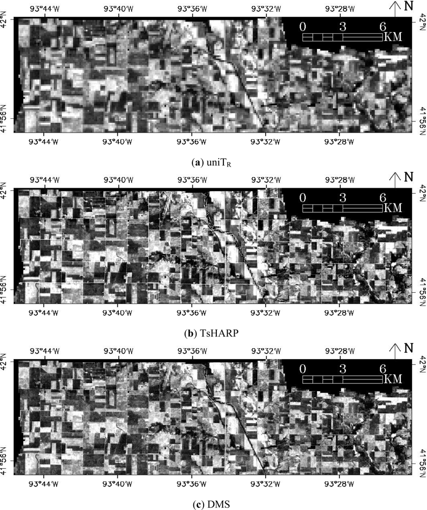
Evaluation of the sharpening techniques for the irrigated site was conducted using Landsat ETM+ data acquired on 22 September 2002. The original 60 m resolution ETM+ TOA brightness temperature image was aggregated to 120 and 240 m. These temperatures were used as references for evaluating T fields sharpened from 960 m resolution. Irrigation significantly influenced the relationships between T-fc or T-R for the entire scene; hence, the local moving windows became more important in the sharpening process. The local window limited the application area and was able to more effectively separate the T-R relationship for the irrigated and non-irrigated fields. In order to account for the variability of temperature caused by irrigation, a smaller window size (10 by 10 pixels in TIR image) was defined in the case study. In Table 7, the statistics associated with these tests are listed for the agricultural subset region (see Figure 7), showing results from both the sharpening models before and after incorporating the residuals and uniTR. The TsHARP and DMS outperformed uniTR, having lower MAE values of 0.5 K and 0.7 K, respectively. Although MAE and r2 values for TsHARP and DMS were similar after incorporating the residuals, the DMS model had a lower MAE value, ∼0.4 K on average, prior to introducing the residuals. This indicates that the underlying T-R formulation used in the DMS model better captured sub-pixel temperature variations caused by land use features other than fractional vegetation cover.
Figure 7 shows T images sharpened from 960 to 6 m by applying uniTR, TsHARP and DMS over a subset of the irrigated Landsat scene. In general, both TsHARP and DMS capture the spatial variability in T compared to the reference T field. The DMS outperformed TsHARP for the irrigated fields in several locations. This can be observed clearly in the inset region (red rectangle in Figure 7a) which is illustrated in Figure 8. In Figure 8(a), two small circular fields (labeled as “1” and “2”) show the typical relationship between T and fc (i.e., higher fc associated with lower surface temperature). However, in the fields recently irrigated—namely the three large circular fields (labeled as “3”, “4” and “5”)—the typical T-fc relationship does not hold. The sparsely vegetated areas in fields 3–5 (low NDVI in Figure 8(b)) show lower temperatures (∼18 °C) compared to densely vegetated area in the reference image (>19 °C) in Figure 8(c). The TsHARP approach produced similar spatial variability of T compared to reference T for the two small circular fields but could not reliably reproduce T for three larger circular fields that were recently irrigated. The DMS model yielded lower errors in the sharpened T image for the irrigated fields, especially for field “4”. This can be attributed to two factors related to the DMS approach. First, the regression tree in the DMS model derived unique T-R relationships for the irrigated and non-irrigated areas, resulting in better predictions of the sharpened T field. Second, the local moving windows in DMS were only applied to a smaller application area and thus the predictions were not affected by different T-R relationships outside the application area. Scatter plots between reference and uniTR, TsHARP, and DMS derived T in Figure 8 further demonstrate the superior performance of the DMS in reproducing high resolution T fields over this scene. The outliers in the TsHARP scatter plot were due to the poor predictions for the three large irrigated (3, 4 and 5 center pivot) fields.
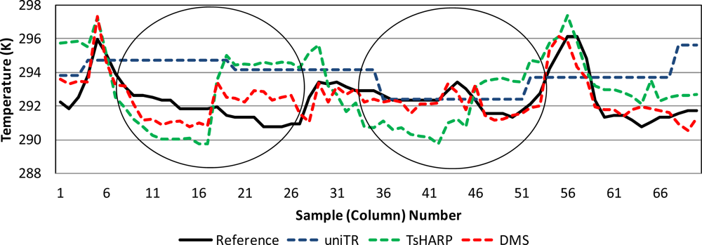
The profile plots (extracted from the pixels along the dashed line in Figure 8(a)) in Figure 9 further demonstrate characteristic errors from the two sharpening approaches and uniTR. The circles in Figure 9 show approximate locations for fields “3” and “4”. Along the x-axis, DMS predictions are closer to the reference T profile. Both TsHARP and DMS miss the decreasing trend in the reference T across field “3”, but the DMS model yields smaller errors. For field “4”, the DMS captures the variability in T while TsHARP estimates deviate significantly from the reference.
Figures 7–9 demonstrate sharpening of LST at a native resolution of 960 m to 60 m resolution. This is close to the TIR sharpening for MODIS resolution imagery (16), which represents an even greater challenge. A major difficulty in applying such large sharpening ratios is that representative homogeneous samples are hard to obtain, since a typical agricultural field size is normally a sub-pixel at the MODIS LST resolution (∼1 km). For sharpening Landsat TIR imagery, the homogeneous pixel criterion (Equation (1)) for developing the T-R relationships is much easier to satisfy. This ensures that enough representative samples are available to provide adequate training data. Figure 10 demonstrates DMS sharpening results at sharpening ratios associated with Landsat TM and ETM+. As reference T at 30 m resolution is not available for this site, the sharpening tests were performed for visual evaluation only. In this test, the standard Landsat ETM+ (60 m) thermal band product, resampled to a 30 m grid by USGS EROS data center, is included for comparison purposes. In addition, this field was aggregated to 120 m then re-sampled to 30 m using nearest neighbor and cubic convolution approaches, approximating data fields that might be generated with Landsat TM (120 m). In the simulated TIR band sharpening tests for TM, both T-R regression (Figure 10(e)) and DMS sharpening (Figure 10(f)) result in well-defined field boundaries and consistent within-field variability of temperature as compared to the original USGS LST data. Although there is no reference temperature for validating the sharpening results, both methods visually outperformed traditional resampling methods, and the sharpening experiment from 960 to 60 m (Figure 8(f)).
4.4. Results from the Complex Terrain Site
Landsat TM data over the complex terrain site in Alaska, acquired on 5 July 2009, were also used to test the TsHARP and DMS thermal sharpening techniques. Table 8 lists statistics evaluating the the performance of these methods when applied to T data at native resolutions 240 m, 480 m, and 960 m resolution and sharpened to 120 m. Again, the DMS outperforms TsHARP by all measures, yielding lower MAE by 0.10–0.34 K. The underlying T-R algorithm captures significantly more intrinsic temperature variability over this complex scene than does the T-fc relationship used in the TsHARP model, yielding lower MAE by 3.17 to 3.86 K before reintroduction of residuals.
A subset of this Landsat scene is illustrated in Figure 11, showing images sharpened from 960 m to 120 m pixel resolution. Thin clouds are visible in the RGB composite image (Figure 11(a)) and the reference temperature image for this region (Figure 11(b)), but are not obvious in the NDVI image (Figure 11(c)). The T-fc (or T-NDVI) relationship cannot capture the temperature variations caused by the thin clouds (Figure 11(e)), which led to the box-like anomalies after applying the residuals as shown in Figure 11(h). The T-R relationship captured the most spatial variation in T in this area (Figure 11(f)), and the DMS-sharpened T (Figure 11(i)) is more consistent with the reference T image (Figure 11(c)), with no obvious box-like anomalies due to large residuals. Some speckling in the final DMS sharpened image may due to the complex relationship between T and shortwave spectral reflectances in this areas that cannot be fully described by regression trees.
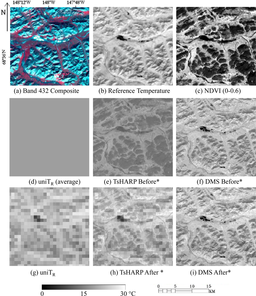
In Figure 12 another subset of this same scene is displayed, in an area of rugged terrain. In this area, effects of topographical shadowing appear in both the RGB composite image (Figure 12(a)) and the TIR image (Figure 12(b)). However, these features are lost in the NDVI image, which samples red-NIR band differences (Figure 12(c)). Consequently the T-fc relationship used in the TsHARP model could not capture the sub-pixel variations in T due to terrain shadowing in this area (Figure 12(e)). This again produced obvious box-like anomalies in the final sharpened T image (Figure 12(h)). The T-R data mining approach captured most of the variability in T due to topographic shadowing (Figure 12(f)) and as a result the DMS model yields a superior sharpened T product (Figure 12(i)). As with the sub-scene in Figure 11, some speckling in the DMS sharpened image in Figure 12 may be due to the fact that sub-pixel variability in T cannot be fully described by spectral reflectance in this area of rugged terrain. Additional information from a digital elevation model, such as hill shade relief, may improve these results and can be easily incorporated into the DMS modeling system.
5. Discussion
Most thermal band image sharpening techniques rely on a biophysical functional relationship between temperature and reflectance or a reflectance-derived index such as NDVI [3,17]. These relationships are described using either linear or non-linear functions. The selection of an appropriate function depends on the experiment site and imagery acquisition dates. Furthermore, simple indices such as NDVI do not capture several factors driving variability in LST, such as variations in senescent vegetation cover, topographic shading, thin clouds, and subpixel moisture variations [18,21–24].
A traditional NDVI-based sharpening approach, TsHARP, has been shown to work well for vegetated areas having relatively uniform weather and soil moisture conditions, as often exist in rainfed agricultural regions during the growing season [3,17]. However, this study has demonstrated that TsHARP is less reliable over non-vegetated areas, irrigated areas, or for imagery acquired during periods dominated by senescent vegetation. This poor performance is due to weak or non-unique functional relationships between T and NDVI that exist under such circumstances [13,18,21,22].
The proposed data mining sharpener (DMS) approach develops T-R relationships based on intrinsic data characteristics and does not rely on any predetermined functional form between T and R. Data mining therefore has potential to be applied operationally for different landscapes and seasons without extensive a priori information regarding scene conditions.
For all test areas considered here—a rainfed agricultural scene, an irrigated agricultural scene, and heterogeneous scene with natural vegetation and rugged terrain—the DMS approach outperformed both TsHARP and a resampling technique involving no sharpening (uniTR), which served as a reference. For each of these three sites, respectively, DMS reduced MAE by 0.15, 0.18 and 0.19 K in comparison with TsHARP, and by 0.35, 0.70 and 0.21 K in comparison with uniTR. Furthermore, in each case the underlying T-R relationship derived by DMS significantly outperformed the T-fc relationship used in TsHARP. This is reflected by the magnitude of residuals between the observed coarse-scale T and the aggregated T retrieved from the relationship assumed in approach, and by the MAE obtained from each sharpening procedure prior to the reintroduction of residuals. Prior to reintroduction, the DMS T-R relationship yields MAE approximately 0.8, 0.4 and 3.5 K less than that from the TsHARP T-fc relationship for each of the three study areas, respectively. This resulted in a notable reduction in box-like anomalies when residuals were incorporated back into the sharpened T fields. This reduction was especially apparent in areas containing irrigated crops, water surfaces, thin cloud cover or areas having significant terrain causing topographic shadowing. Similar results were reported by Merlin et al.[22], who found box-like anomalies were reduced by incorporating effects of non-photosynthetic material in conjunction with the green biomass information conveyed by NDVI.
These case studies showed that the suite of spectral band reflectances sampled by Landsat contain more information than does NDVI relating to spatial variations in land-surface temperature. In general, local regression models built from small moving windows were more accurate than the global models built on samples selected from the whole scene, as reported by Jeganathan et al.[23]. However, the global model derived for the whole scene may provide better sharpening results for small objects that are not sampled by the local sampling window. The combination of local and global T-R formulations provides a practical approach for thermal sharpening within the DMS modeling framework.
6. Conclusions
Thermal infrared (TIR) band imagery provides key information for mapping land surface energy fluxes and evapotranspiration, and for monitoring crop stress. While land-surface temperature data at fine resolution are required for field scale applications, TIR imagery is normally acquired at a coarser pixel resolution compared to shortwave spectral bands. A robust data mining sharpening (DMS) approach has been developed to sharpen TIR imagery using spectral band reflectances, using a cubist regression tree method to develop functional relationships between temperature (T) and reflectance (R). Both local and global temperature and reflectance formulations are combined within the DMS processing framework. In comparison with a classic sharpening technique (TsHARP), DMS outperformed TsHARP in each of three test areas representing rainfed agriculture, irrigated agriculture and a site with natural vegetation and complex terrain. The mean absolute errors (MAE) in DMS retrievals for the rainfed agricultural site vary from 0.35 to 1.24 K for sharpening ratios of 2 to 16, representing the ratio between the resolution of the shortwave and TIR band sensors. For the irrigated site, MAE varies from 0.58 to 0.80 K for sharpening ratios of 4 to 16. Slightly higher MAE values (0.78 to 1.67) are obtained for the complex terrain site for sharpening ratios from 2 to 8. A notable reduction in box-like anomalies resulting from energy conservation enforcement is obtained when T residuals are incorporated, especially for the irrigated agriculture and complex terrain sites.
The analyses of the sharpening techniques described in this paper were conducted using land surface temperature and reflectance data collected from the same platform and represent the best-case scenario in terms of accuracy in the sharpened temperature maps. The application of data mining to T and R from different satellite platforms may be affected by several additional factors such as the geo-referencing accuracy, the number of spectral bands available for sharpening, the date/time differences, and differences in data quality, yielding actual errors larger than those found from the simulated tests in this paper. Further investigations are planned to evaluate the DMS using combinations of TIR and shortwave reflectances from different sensor platforms, such as the Geostationary Operational Environmental Satellites (GOES) and the Moderate Resolution Imaging Spectroradiometer (MODIS) spectral band reflectance, or sharpening MODIS temperature using Landsat or Landsat-like spectral band reflectances. The latter approach would be useful for generating dense time-series temperature data at sub-field spatial resolutions for applications in water resource monitoring.
Development of a refined DMS approach that is less computationally intensive and can be applied routinely and operationally to real time imagery from Landsat and MODIS is in progress. Future papers will describe the framework for an operational DMS system, along with evaluation over a variety of landscapes and climatic regions. Because the DMS uses reflectance data as independent variables and does not depend on high order products (e.g. land cover, albedo and emissivity) as used in other sharpening approaches[13,20–22], the DMS framework is more flexible and adaptable for automated operational data production. Additional ancillary data (e.g., terrain, soil moisture) can be easily incorporated in the processing if deemed necessary for specific sites or climates.
Sharpening thermal band imagery using spectral band reflectance provides an inexpensive means for obtaining thermal band imagery at finer resolutions. However, these sharpening approaches cannot provide information that is required to fully describe the sub-pixel variability in LST at coarser resolutions and will always contain some level noise and inaccuracies, which may be a critical limitation for monitoring land surface fluxes and vegetation conditions at the field and sub-field scales. Additional ancillary information such as high resolution soil moisture and hill shade relief may be useful for improving model prediction. Nevertheless, thermal sharpening techniques cannot replace actual thermal imagery at fine resolutions or missions that provide high quality thermal band imagery at high temporal and spatial resolution critical for many land and water resource management applications.
Acknowledgments
This work was supported by the US Geological Survey (USGS) Landsat Data Continuity Mission (LDCM) Science Team program and the NASA Earth Observing System (EOS) program. Special thanks to Christopher Neale and Nurit Agam for providing airborne thermal imagery used in this study.
References
- Justice, C.O.; Giglio, L.; Korontzi, S.; Owens, J.; Morisette, J.T.; Roy, D.; Descloitres, J.; Alleaume, S.; Petitcolin, F.; Kaufman, Y. The MODIS fire products. Remote Sens. Environ 2002, 83, 244–262. [Google Scholar]
- Harris, S.; Veraverbeke, S.; Hook, S. Evaluating spectral indices for assessing fire severity in Chaparral Ecosystems (Southern California) Using MODIS/ASTER (MASTER) airborne simulator data. Remote Sens 2011, 3, 2403–2419. [Google Scholar]
- Kustas, W.P.; Norman, J.M.; Anderson, M.C.; French, A.N. Estimating subpixel surface temperatures and energy fluxes from the vegetation index-radiometric temperature relationship. Remote Sens. Environ 2003, 85, 429–440. [Google Scholar]
- Norman, J.M.; Anderson, M.C.; Kustas, W.P.; French, A.N.; Mecikalski, J.; Torn, R.; Diak, G.R.; Schmugge, T.J.; Tanner, B.C.W. Remote sensing of surface energy fluxes at 10-m pixel resolutions. Water Resour. Res 2003, 39, 1221–1238. [Google Scholar]
- Kustas, W.P.; Li, F.; Jackson, T.J.; Prueger, J.H.; MacPherson, J.I.; Wolde, M. Effects of remote sensing pixel resolution on modeled energy flux variability of croplands in Iowa. Remote Sens. Environ 2004, 92, 535–547. [Google Scholar]
- Anderson, M.C.; Norman, J.M.; Mecikalski, J.R.; Torn, R.D.; Kustas, W.P.; Basara, J.B. A multi-scale remote sensing model for disaggregating regional fluxes to micrometeorological scales. J. Hydrometeorol 2004, 5, 343–363. [Google Scholar]
- Anderson, M.C.; Kustas, W.P.; Norman, J.M. Upscaling flux observations from local to continental scales using thermal remote sensing. Agron. J 2007, 99, 240–254. [Google Scholar]
- Anderson, M.C.; Norman, J.M.; Kustas, W.P.; Houborg, R.; Starks, P.J.; Agam, N. A thermal-based remote sensing technique for routine mapping of land-surface carbon, water and energy fluxes from field to regional scales. Remote Sens. Environ 2008, 112, 4227–4241. [Google Scholar]
- Anderson, M.C.; Kustas, W.P.; Norman, J.M.; Hain, C.R.; Mecikalski, J.R.; Schultz, L.; Gonzalez-Dugo, M.P.; Cammalleri, C.; d’Urso, G.; Pimstein, A.; Gao, F. Mapping daily evapotranspiration at field to continental scales using geostationary and polar orbiting satellite imagery. Hydrol. Earth Syst. Sci 2011, 15, 223–239. [Google Scholar] [Green Version]
- Allen, R.G.; Tasumi, M.; Morse, A.; Trezza, R. A Landsat-based energy balance and evapotranspiration model in Western US water rights regulation and planning. J. Irrig. Drain. Syst 2005, 19, 251–268. [Google Scholar]
- Voogt, J.A.; Oke, T.R. Thermal remote sensing of urban climates. Remote Sens. Environ 2003, 86, 370–384. [Google Scholar]
- Quattrochi, D.A.; Luvall, J. (Eds.) Thermal Remote Sensing in Land Surface Processes; CRC Press, Taylor and Francis: Boca Raton, FL, USA, 2004.
- Dominguez, A.; Kleissl, J.; Luvall, J.C.; Rickman, D.L. High-resolution urban thermal sharpener (HUTS). Remote Sens. Environ 2011, 115, 1772–1780. [Google Scholar]
- Liu, L.; Zhang, Y. Urban heat island analysis using the Landsat TM data and ASTER data: A case study in Hong Kong. Remote Sens 2011, 3, 1535–1552. [Google Scholar]
- Rinner, C.; Hussain, M. Toronto’s Urban Heat Island—Exploring the relationship between land use and surface temperature. Remote Sens 2011, 3, 1251–1265. [Google Scholar]
- Moran, M.S.; Clarke, T.R.; Inoue, Y.; Vidal, A. Estimating crop water deficit using the relation between surface-air temperature and spectral vegetation index. Remote Sens. Environ 1994, 49, 246–263. [Google Scholar]
- Agam, N.; Kustas, W.P.; Anderson, M.C.; Li, F.; Neale, C.M.U. A vegetation index based technique for spatial sharpening of thermal imagery. Remote Sens. Environ 2007, 107, 545–558. [Google Scholar]
- Agam, N.; Kustas, W.P.; Anderson, M.C.; Li, F.; Colaizzi, P.D. Utility of thermal sharpening over Texas high plains irrigated agricultural fields. J. Geophys. Res 2007, 112, D19110. [Google Scholar]
- Anderson, M.C.; Neale, C.M.U.; Li, F.; Norman, J.M.; Kustas, W.P.; Jayanthi, H.; Chavez, J. Upscaling ground observations of vegetation water content, canopy height, and leaf area index during SMEX02 using aircraft and Landsat imagery. Remote Sens. Environ 2004, 92, 447–464. [Google Scholar]
- Inamdar, A.K.; French, A.; Hook, S.; Vaughan, G.; Luckett, W. Land surface temperature retrieval at high spatial and temporal resolutions over the southwestern United States. J. Geophys. Res 2008, 113, D07107. [Google Scholar]
- Inamdar, A.K.; French, A. Disaggregation of GOES land surface temperatures using surface emissivity. Geophys. Res. Lett 2009, 36, D02408. [Google Scholar]
- Merlin, O.; Duchemin, B.; Hagolle, O.; Jacob, F.; Coudert, B.; Chehbouni, G.; Dedieu, G.; Garatuza, J.; Kerr, Y. Disaggregation of MODIS surface temperature over an agricultural area using a time series of Formosat-2 images. Remote Sens. Environ 2010, 114, 2500–2512. [Google Scholar] [Green Version]
- Jeganathan, C.; Hamm, N.A.S.; Mukherjee, S.; Atkinson, P.M.; Raju, P.L.N.; Dadhwal, V.K. Evaluating a thermal image sharpening model over a mixed agricultural landscape in India. Int. J. Appl. Earth Obs 2011, 13, 178–191. [Google Scholar]
- Chen, X.; Yamaguchi, Y.; Chen, J.; Shi, Y. Scale effect of vegetation-index-based spatial sharpening for thermal imagery: A simulation study by ASTER data. IEEE Geosci. Remote Sens. Lett 2012, 9, 549–553. [Google Scholar]
- Zakšek, K.; Oštir, K. Downscaling land surface temperature for urban heat island diurnal cycle analysis. Remote Sens. Environ 2012, 117, 114–124. [Google Scholar]
- Quinlan, J.R. Learning with Continuous Classes. Proceedings of 5th Australian Joint Conference on Artificial Intelligence, Hobart, Tasmania, 16–18 November 1992; pp. 343–348.
- Quinlan, J.R. Rulequest Data Mining Tools. Available online: http://www.rulequest.com/ (accessed on 10 October 2012).
- Menenti, M.; Bastiaanssen, W.; van Eick, D.; Abd el Karim, M.A. Linear relationships between surface reflectance and temperature and their application to map actual evaporation of groundwater. Adv. Space Res 1989, 9, 165–176. [Google Scholar]
- Yang, G.; Pu, R.; Huang, W.; Wang, J.; Zhao, C. A novel method to estimate subpixel temperature by fusing solar-reflective and thermal-infrared remote-sensing data with an artificial neural network. IEEE Trans. Geosci. Remote Sens 2010, 48, 2170–2178. [Google Scholar]
- Karnieli, A.; Agam, N.; Pinker, R.T.; Anderson, M.C.; Imhoff, M.L.; Gutman, G.G.; Panov, N.; Goldberg, A. Use of NDVI and land surface temperature for drought assessment: Merits and limitations. J. Climate 2010, 23, 618–633. [Google Scholar]
- Masek, J.G.; Vermote, E.F.; Saleous, N.E.; Wolfe, R.; Hall, F.G.; Huemmrich, F.; Gao, F.; Kutler, J.; Lim, T.K. A Landsat surface reflectance data set for North America, 1990–2000. IEEE Geosci. Remote Sens. Lett 2006, 3, 69–72. [Google Scholar]
- Li, F.; Jackson, T.J.; Kustas, W.P.; Schmugge, T.J.; French, A.N.; Cosh, M.H.; Bindlish, R. Deriving land surface temperature from Landsat 5 and 7 during SMEX02/SMACEX. Remote Sens. Environ 2004, 92, 521–534. [Google Scholar]
- Liu, Y.; Hiyama, T.; Yamaguchi, Y. Scaling of land surface temperature using satellite data: A case examination of ASTER and MODIS products over a heterogeneous terrain area. Remote Sens. Environ 2006, 105, 115–128. [Google Scholar]
- Schott, J.; Gerace, A.; Brown, S.; Gartley, M.; Montanaro, M.; Reuter, D. Simulation of image performance characteristics of the Landsat data continuity mission (LDCM) thermal infrared sensor (TIRS). Remote Sens 2012, 4, 2477–2491. [Google Scholar]
Figure 1.
Data processing flow chart (clear boxes represent data and shaded boxes represent processing procedures).
Figure 1.
Data processing flow chart (clear boxes represent data and shaded boxes represent processing procedures).

Figure 2.
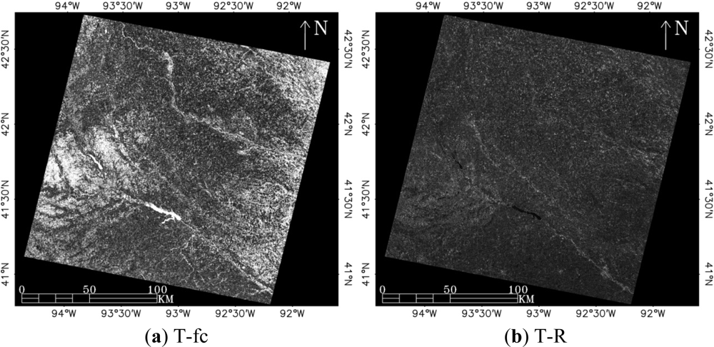
Absolute difference (residuals) between model predictions and reference temperatures at 60 m resolution for the rainfed agricultural site (Landsat WRS-2 path 26 and row 31) on 14 May (a,b), 1 July (c,d) and 22 November (e,f). The first column shows the T-fc model prediction from TsHARP and second column shows the global T-R model prediction from the data mining sharpener (DMS). Images were sharpened from 240 to 60 m pixel resolution.
Figure 2.
Absolute difference (residuals) between model predictions and reference temperatures at 60 m resolution for the rainfed agricultural site (Landsat WRS-2 path 26 and row 31) on 14 May (a,b), 1 July (c,d) and 22 November (e,f). The first column shows the T-fc model prediction from TsHARP and second column shows the global T-R model prediction from the data mining sharpener (DMS). Images were sharpened from 240 to 60 m pixel resolution.


Figure 3.
Application of the local model, the global model and combined model in a subset window (3 km by 3 km) within the rainfed agricultural site shown in the composite image in (a) for 14 May 2002. The reference temperature (b) is shown in 60 m pixel resolution. Images from the local model (c), the global model (d) and combined model (e) were sharpened from 240 to 60 m pixel resolution. Weights for the local model are shown in (f).


Figure 4.
Sharpening results from uniTR, TsHARP and DMS as compared to the Landsat ETM+ reference temperature in a subset window (24 km by 24 km) over the rainfed agricultural site. The top row shows ETM+ reference temperature at 60 m resolution. Results from uniTR (no sharpening), TsHARP and DMS are shown in 2nd, 3rd and bottom rows respectively. Three columns show Landsat imaging dates 14 May, 1 July and 22 November respectively. The TsHARP and DMS images were sharpened from 240 m to 60 m pixel resolution, while uniTr is at 240 m resolution.

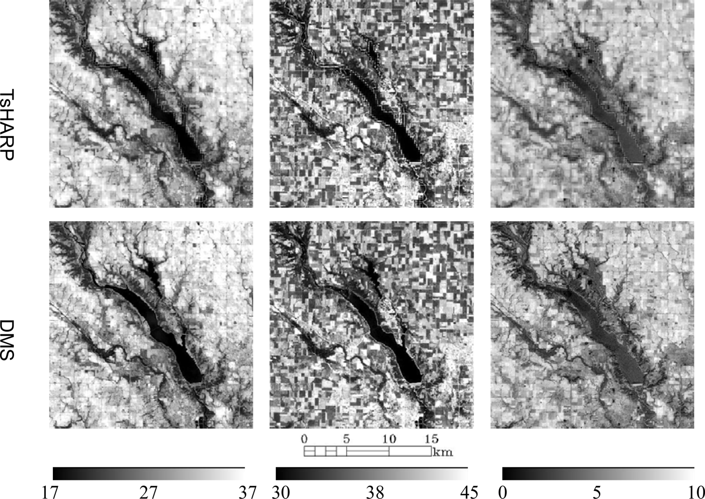
Figure 5.
Applications of uniTR (a), TsHARP (b) and DMS (c) to airborne TIR imagery from 1 July 2002 aggregated to 120 m and sharpened to 30 m, compared to a reference temperature field at 30 m (d).
Figure 5.
Applications of uniTR (a), TsHARP (b) and DMS (c) to airborne TIR imagery from 1 July 2002 aggregated to 120 m and sharpened to 30 m, compared to a reference temperature field at 30 m (d).


Figure 6.
Applications of uniTR, TsHARP, and DMS to simulated 120 m data from two sources (airborne and ETM+) both acquired on 1 July 2002 in a subset area (2.4 km by 2.2 km, center in Figure 5) of the SMACEX’02 campaign site. The reference temperature (a,b) is shown in 30 m pixel resolution. Images from uniTR (c,d), TsHARP (e,f) and DMS (g,h) were sharpened from 120 to 30 m pixel resolution. The first column shows results from airborne data and second column shows results from Landsat.
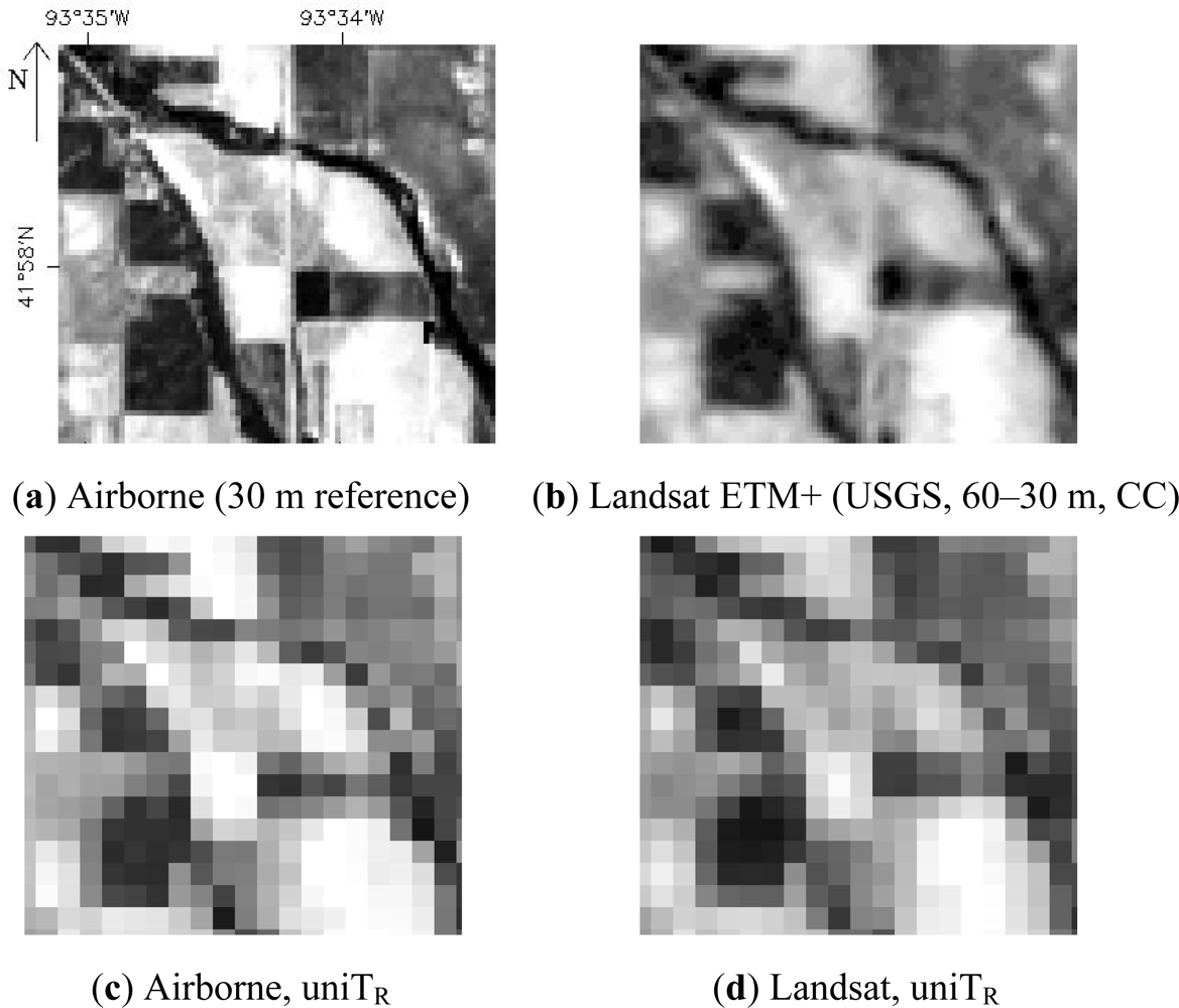
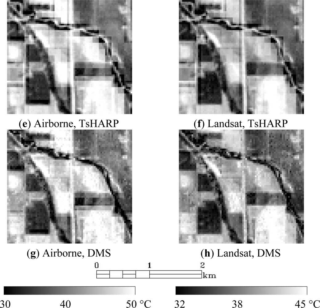
Figure 7.
Applications of uniTR, TsHARP and DMS to a subset irrigated agricultural area (72 km by 36 km) as compared to the reference temperature (a) in 60 m resolution. Images from uniTR (b), TsHARP (c) and DMS (d) were sharpened from 960 to 60 m pixel resolution.
Figure 7.
Applications of uniTR, TsHARP and DMS to a subset irrigated agricultural area (72 km by 36 km) as compared to the reference temperature (a) in 60 m resolution. Images from uniTR (b), TsHARP (c) and DMS (d) were sharpened from 960 to 60 m pixel resolution.
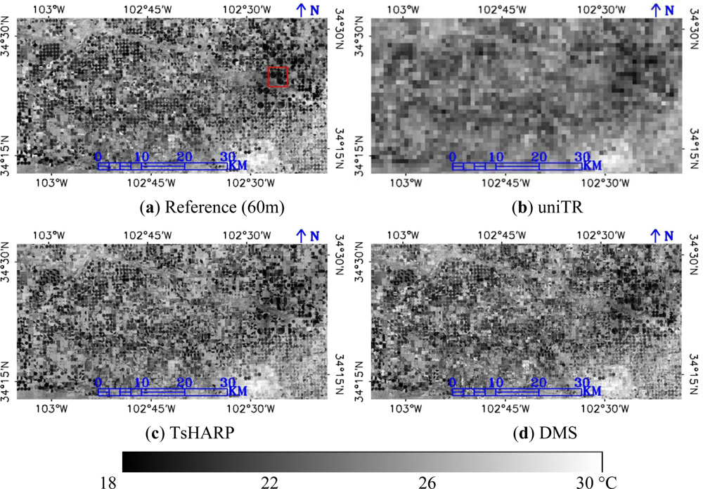
Figure 8.
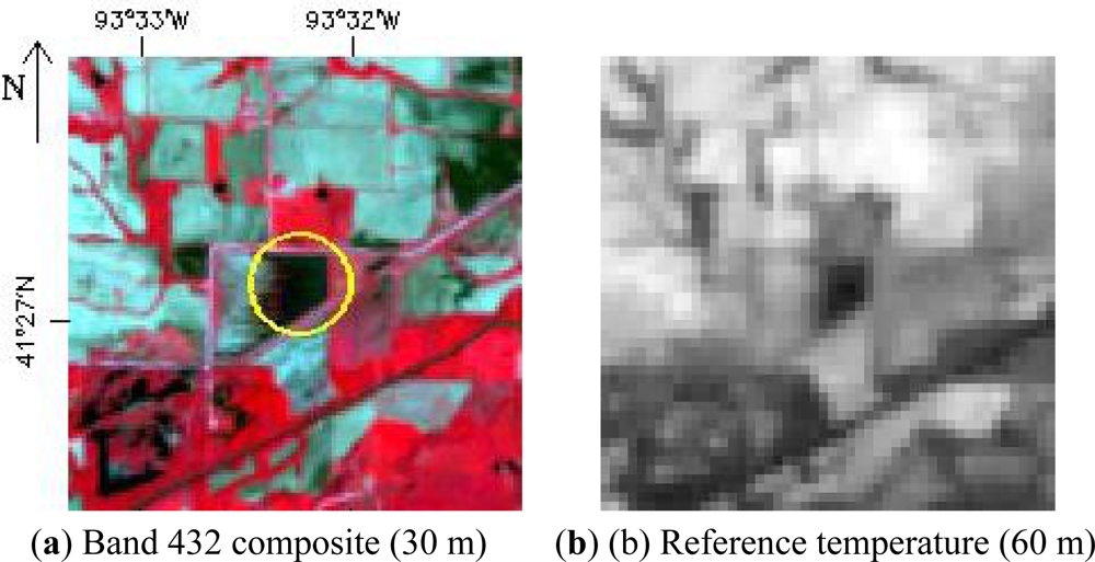
A zoomed view of the area within the red rectangle (4.3 km by 4.3 km) in Figure 7 showing composite reflectance (a), NDVI (b), and reference temperature (c) at 60 m resolution. Sharpening results (960 to 60 m) from uniTR (d), TsHARP (e) and DMS (f) are compared to the reference temperatures and are shown in scatter plots (g), (h) and (i), respectively.
Figure 8.
A zoomed view of the area within the red rectangle (4.3 km by 4.3 km) in Figure 7 showing composite reflectance (a), NDVI (b), and reference temperature (c) at 60 m resolution. Sharpening results (960 to 60 m) from uniTR (d), TsHARP (e) and DMS (f) are compared to the reference temperatures and are shown in scatter plots (g), (h) and (i), respectively.
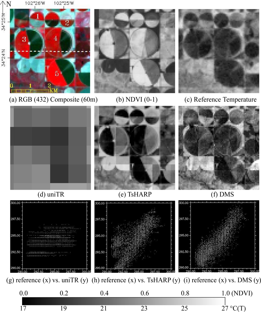
Figure 9.
X-axis profile of temperature shows DMS (red) outperformed uniTR (blue) and TsHARP (green) in capturing spatial variation of temperature (black, reference) for the dashed line in Figure 8(a). The two ovals from left to right refer to the sample pixels extracted from fields 3 and 4, respectively.

Figure 10.
Application of DMS using simulated Landsat TM 120 m thermal band and 30 m shortwave bands. The sharpened results from the subset area (a) (same as Figure 8) show clear field boundaries and within field variation compared to traditional resampling methods (b,c) (NN: nearest neighbor; CC: cubic convolution) and original T (d) from the US Geological Survey (USGS) Earth Resources Observation and Science (EROS) data center (re-sampled to 30 m from 60 m ETM+ data). The T-R prediction and DMS result are shown in (e) and (f) respectively.
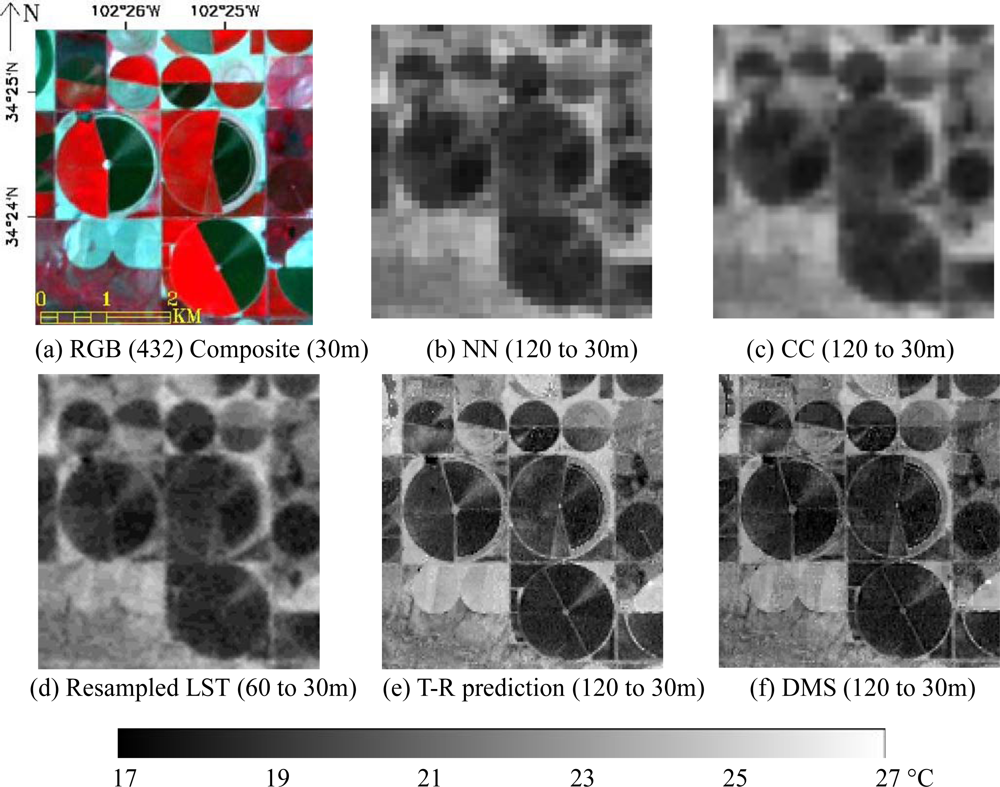
Figure 11.
Sharpened results from uniTR, TsHARP and DMS (960 to 120 m) for a subset area (23.8 km by 23.2 km) contaminated by thin clouds. Thin clouds can be observed in the RGB composite (a) and the reference temperature field (b), but are not obvious in NDVI (c) (all at 120 m). The model predictions from the three approaches are shown in (d–f). The uniTR approach does not include sharpening model and is shown in average value. The final results after redistributing residuals are shown in (g–i). (*Before and After refer to before and after incorporating residuals in the two sharpening models, TsHARP and DMS).
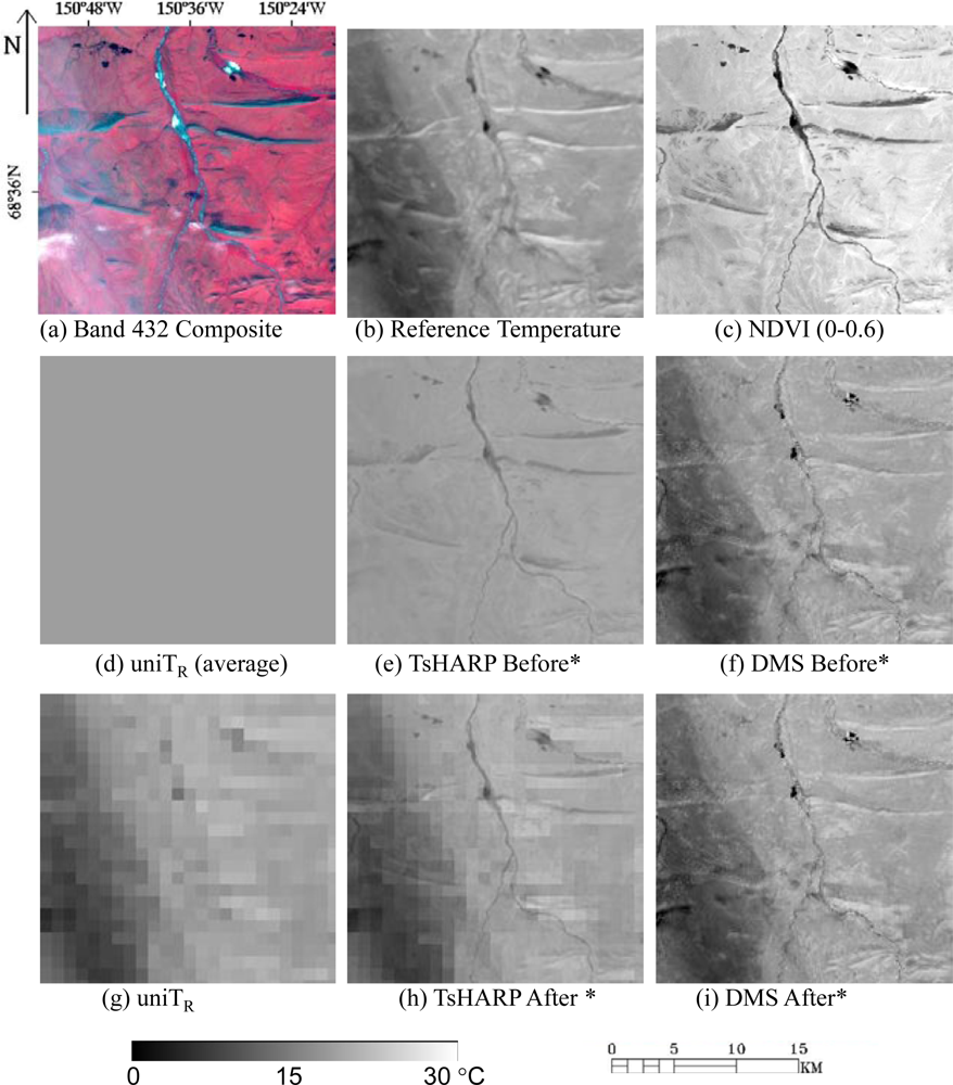
Figure 12.
Sharpened results from uniTr, TsHARP and DMS (960 to 120 m) for a subset area impacted by rugged terrain (23.8 km by 23.2 km). Topographic shadowing can be observed in the RGB composite (a) and the reference temperature field (b), but is not obvious in NDVI (c) (all at 120 m). The uniTR approach does not include sharpening model and is shown in average value (d). The sharpened T field predictions before incorporating the residuals are shown in (e) and (f). The results using uniTR (g) and after redistributing residuals for TsHARP and DMS are shown in (h) and (i), respectively. (*Before and After refer to before and after incorporating residuals in the two sharpening models, TsHARP and DMS).

Table 1.
Spatial resolutions of typical medium resolution sensors for shortwave spectral bands and thermal infrared (TIR) bands, along with ratio of TIR and shortwave band resolution.
| Sensor | Shortwave (m) | TIR (m) | Ratio |
|---|---|---|---|
| Landsat TM | 30 | 120 | 4 |
| Landsat ETM+ | 30 | 60 | 2 |
| LDCM (TIRS+OLI) | 30 | 90 | 3 |
| Terra ASTER | 15–30 | 90 | 4–6 |
Table 2.
Test sites and data used in the case studies. TIR datasets were aggregated to set of simulated coarse resolutions, and sharpened to finer resolutions (typically the native resolution of the TIR dataset).
| Test Site | Sensor | WRS2 Path-Row | Date | Mean LST (°C) | Standard Deviation (°C) | Mean NDVI | Simulated Coarse TIR Resolution (m) | Reference Resolution (m) |
|---|---|---|---|---|---|---|---|---|
| Rainfed | ETM+ | p26r31 | 05/14/02 | 27.3 | 4.0 | 0.38 | 120,240,480,960 | 60 |
| ETM+ | p26r31 | 07/01/02 | 36.9 | 3.4 | 0.64 | 120,240,480,960 | 60 | |
| ETM+ | p26r31 | 11/22/02 | 5.5 | 1.7 | 0.24 | 120,240,480,960 | 60 | |
| airborne | Subset | 07/01/02 | 37.5 | 3.3 | - | 120 | 30 | |
| Irrigated | ETM+ | p31r36 | 09/22/02 | 24.8 | 2.5 | 0.35 | 960 | 60,120,240 |
| Natural | TM | p73r12 | 07/05/09 | 15.1 | 8.9 | 0.34 | 240,480,960 | 120 |
Table 3.
Values of Mean Absolute Error (MAE) and r2 from comparisons of the T-fc and T-R (local and global) models, applied at 4 sharpening ratios, with reference temperature data from three dates over the rain fed agricultural site (unit: °C or K)
| Date | 14 May 2002 | 1 July 2002 | 22 November 2002 | ||||||
|---|---|---|---|---|---|---|---|---|---|
| Resolution | T-fc | T-R (global) | T-R (local) | T-fc | T-R (global) | T-R (local) | T-fc | T-R (global) | T-R (local) |
| Mean Absolute Error | |||||||||
| 120 to 60 m | 2.13 | 1.44 | 0.99 | 1.48 | 0.99 | 0.72 | 1.26 | 0.67 | 0.55 |
| 240 to 60 m | 2.14 | 1.47 | 1.11 | 1.50 | 1.03 | 0.81 | 1.26 | 0.70 | 0.60 |
| 480 to 60 m | 2.14 | 1.56 | 1.24 | 1.53 | 1.09 | 0.91 | 1.26 | 0.76 | 0.66 |
| 960 to 60 m | 2.15 | 1.75 | 1.42 | 1.61 | 1.23 | 1.10 | 1.26 | 0.81 | 0.70 |
| Coefficient of Determination (r2) | |||||||||
| 120 to 60 m | 0.47 | 0.78 | 0.80 | 0.58 | 0.85 | 0.92 | 0.08 | 0.73 | 0.81 |
| 240 to 60 m | 0.47 | 0.77 | 0.86 | 0.58 | 0.85 | 0.90 | 0.08 | 0.71 | 0.78 |
| 480 to 60 m | 0.47 | 0.74 | 0.83 | 0.60 | 0.83 | 0.88 | 0.08 | 0.67 | 0.74 |
| 960 to 60 m | 0.47 | 0.67 | 0.78 | 0.62 | 0.82 | 0.84 | 0.08 | 0.64 | 0.72 |
Table 4.
Values of MAE in sharpened thermal imagery before and after applying residuals to the TsHARP and DMS models (unit: °C or K).
| 5/14/2002 | 7/1/2002 | 11/22/2002 | ||||
|---|---|---|---|---|---|---|
| Before* | After* | Before | After | Before | After | |
| TsHARP | ||||||
| 120 to 60 m | 2.13 | 0.56 | 1.48 | 0.58 | 1.26 | 0.37 |
| 240 to 60 m | 2.14 | 0.87 | 1.50 | 0.83 | 1.26 | 0.59 |
| 480 to 60 m | 2.14 | 1.14 | 1.53 | 1.05 | 1.26 | 0.79 |
| 960 to 60 m | 2.15 | 1.36 | 1.61 | 1.28 | 1.26 | 0.94 |
| DMS | ||||||
| 120 to 60 m | 0.91 | 0.56 | 0.68 | 0.47 | 0.51 | 0.35 |
| 240 to 60 m | 1.03 | 0.78 | 0.78 | 0.64 | 0.58 | 0.48 |
| 480 to 60 m | 1.18 | 1.00 | 0.90 | 0.78 | 0.65 | 0.59 |
| 960 to 60 m | 1.38 | 1.24 | 1.08 | 0.97 | 0.70 | 0.65 |
Table 5.
Values of r2 between reference fields and sharpened results after applying residuals to TsHARP and DMS models.
| Date | 5/14/2002 | 7/1/2002 | 11/22/2002 | ||||||
|---|---|---|---|---|---|---|---|---|---|
| Resolution | uniTR | TsHARP | DMS | uniTR | TsHARP | DMS | uniTR | TsHARP | DMS |
| 120 to 60 m | 0.96 | 0.96 | 0.97 | 0.94 | 0.94 | 0.97 | 0.92 | 0.91 | 0.94 |
| 240 to 60 m | 0.88 | 0.91 | 0.94 | 0.81 | 0.88 | 0.95 | 0.78 | 0.76 | 0.88 |
| 480 to 60 m | 0.77 | 0.85 | 0.89 | 0.62 | 0.82 | 0.92 | 0.62 | 0.60 | 0.82 |
| 960 to 60 m | 0.67 | 0.79 | 0.83 | 0.44 | 0.78 | 0.88 | 0.45 | 0.46 | 0.77 |
Table 6.
Statistical comparison of thermal airborne and ETM+ imagery sharpened from 120 to 30 m using uniTR, TshARP and DMS in comparison with the reference airborne field and the resampled ETM+ thermal data at 30 m resolution.
| MAE (°C) | r2 | |||
|---|---|---|---|---|
| Data Source | Airborne | ETM+ | Airborne | ETM+ |
| uniTR | 1.80 | 0.74 | 0.80 | 0.90 |
| TsHARP | 1.58 | 0.76 | 0.85 | 0.90 |
| DMS | 1.42 | 0.63 | 0.87 | 0.94 |
Table 7.
Statistical comparison of reference temperature field at 60, 120 and 240 m with sharpened results from uniTR, TsHARP and DMS before and after incorporating residuals for the irrigated agricultural site (scene subset).
| Resolution | Before* | After* | |||
|---|---|---|---|---|---|
| TsHARP | DMS | uniTR | TsHARP | DMS | |
| MAE (°C or K) | |||||
| 960 to 60 m | 1.29 | 0.91 | 1.49 | 0.95 | 0.80 |
| 960 to 120 m | 1.24 | 0.80 | 1.41 | 0.87 | 0.67 |
| 960 to 240 m | 1.16 | 0.72 | 1.24 | 0.76 | 0.58 |
| r2 | |||||
| 960 to 60 m | 0.56 | 0.77 | 0.45 | 0.76 | 0.83 |
| 960 to 120 m | 0.56 | 0.83 | 0.46 | 0.77 | 0.86 |
| 960 to 240 m | 0.56 | 0.83 | 0.53 | 0.81 | 0.88 |
Table 8.
Statistics of sharpening results from uniTR, TsHARP and DMS before and after residual application for the heterogeneous site.
| Resolution | Before* | After* | |||
|---|---|---|---|---|---|
| TsHARP | DMS | uniTR | TsHARP | DMS | |
| MAE (°C or K) | |||||
| 240 to 120 m | 5.19 | 1.33 | 0.77 | 0.88 | 0.78 |
| 480 to 120 m | 5.19 | 1.66 | 1.40 | 1.36 | 1.22 |
| 960 to 120 m | 5.23 | 2.06 | 2.13 | 2.01 | 1.67 |
| r2 | |||||
| 240 to 120 m | 0.31 | 0.90 | 0.98 | 0.98 | 0.98 |
| 480 to 120 m | 0.31 | 0.86 | 0.92 | 0.92 | 0.94 |
| 960 to 120 m | 0.31 | 0.85 | 0.83 | 0.85 | 0.88 |
Share and Cite
MDPI and ACS Style
Gao, F.; Kustas, W.P.; Anderson, M.C. A Data Mining Approach for Sharpening Thermal Satellite Imagery over Land. Remote Sens. 2012, 4, 3287-3319. https://doi.org/10.3390/rs4113287
AMA Style
Gao F, Kustas WP, Anderson MC. A Data Mining Approach for Sharpening Thermal Satellite Imagery over Land. Remote Sensing. 2012; 4(11):3287-3319. https://doi.org/10.3390/rs4113287
Chicago/Turabian StyleGao, Feng, William P. Kustas, and Martha C. Anderson. 2012. "A Data Mining Approach for Sharpening Thermal Satellite Imagery over Land" Remote Sensing 4, no. 11: 3287-3319. https://doi.org/10.3390/rs4113287