Evaluation of Four Supervised Learning Methods for Benthic Habitat Mapping Using Backscatter from Multi-Beam Sonar


1
School of Life & Environmental Sciences, Faculty of Science and Technology, Deakin University, PO Box 423, Warrnambool, VIC 3280, Australia
2
Razak School of Engineering and Advanced Technology, Universiti Teknologi Malaysia, 54100 Kuala Lumpur, Malaysia
*
Author to whom correspondence should be addressed.
Remote Sens. 2012, 4(11), 3427-3443; https://doi.org/10.3390/rs4113427
Submission received: 27 August 2012
/
Revised: 2 November 2012
/
Accepted: 5 November 2012
/
Published: 12 November 2012
Abstract
:An understanding of the distribution and extent of marine habitats is essential for the implementation of ecosystem-based management strategies. Historically this had been difficult in marine environments until the advancement of acoustic sensors. This study demonstrates the applicability of supervised learning techniques for benthic habitat characterization using angular backscatter response data. With the advancement of multibeam echo-sounder (MBES) technology, full coverage datasets of physical structure over vast regions of the seafloor are now achievable. Supervised learning methods typically applied to terrestrial remote sensing provide a cost-effective approach for habitat characterization in marine systems. However the comparison of the relative performance of different classifiers using acoustic data is limited. Characterization of acoustic backscatter data from MBES using four different supervised learning methods to generate benthic habitat maps is presented. Maximum Likelihood Classifier (MLC), Quick, Unbiased, Efficient Statistical Tree (QUEST), Random Forest (RF) and Support Vector Machine (SVM) were evaluated to classify angular backscatter response into habitat classes using training data acquired from underwater video observations. Results for biota classifications indicated that SVM and RF produced the highest accuracies, followed by QUEST and MLC, respectively. The most important backscatter data were from the moderate incidence angles between 30° and 50°. This study presents initial results for understanding how acoustic backscatter from MBES can be optimized for the characterization of marine benthic biological habitats.
1. Introduction
Quantitative analysis of acoustic backscatter intensity from multibeam echo-sounder (MBES) provides valuable information for mapping of seafloor habitats. The importance of preserving the effect of incidence angle from angular backscatter intensity to characterize seafloor types is well established [1–4]. Although these works have primarily focused on developing models for seafloor sediment characterization, some studies have also incorporated this information for the discrimination of benthic biota [5–9]. Among these, terrestrial classification methods have been applied including; general clustering [8], linear discriminant analysis and principal component analysis [9,10], decision trees [5] and factor analysis [6]. With the multitude of classification approaches available there is a need to compare different algorithms to gain further insights into classifier performance when using acoustic sources.
Generally, angular backscatter from MBES and side scan sonar are a product of two acoustic scattering processes; volume and interface scatterings [11]. Interface scattering is the energy produced at the water-sediment surface. Volume scattering occurs when part of an acoustic signal penetrates the physical structure and is scattered by the heterogeneities in the sedimentary layers. Acoustic scattering can be separated into three main sectors; near nadir, moderate incidence angle and outer angle. For a flat seabed without macro-roughness at near nadir area (near vertical incidence angle), angular backscatter is a product of large scale roughness. By contrast, at moderate incidence angle the backscatter is a combination of the volume inhomogeneity and small scale interface roughness. At the outer incidence angle only small scale roughness is important [12]. Backscatter intensity between incident angles of 30° and 50° is often used to reference backscatter data to remove the angular dependence for creating normalized backscatter images [7]. For distinguishing between soft and hard habitats, the maximum separation of angular backscatter intensity has been observed at an incidence angle of 40° [7]. By using entire angular response curves (e.g., incidence angle between 0° and 70° at one degree intervals), Hamilton and Parnum [8] demonstrated high class separation at moderate incidence angles between 35° and 45° with less discrimination for near nadir angles. The measurements at near nadir have minimum contribution to the discrimination process as these measurements have been found to be mainly dominated by noise [2,6]. However, near nadir and outer angles are still required for the geo-acoustic inversion process and for the construction of a generic model from angular response information [1,3]. This study will assess the interaction of different angular domains for class differentiation.
The characterization process can also use important features from angular curves. Extracting simple characteristics (e.g., mean and slope of angular backscatter intensity) from angular domains [2,13] or parameters by modeling the angular curve as a specific shape distribution [3] can contribute to class differentiation. Parnum and Gavrilov [9] found that the mean angular backscatter between 15° and 45° provided a better discrimination than the slope of angular backscatter (i.e., 15°–45°) for distinguishing rock, sand and rhodolith beds.
Use of a single classification for an entire backscatter response curve may result in habitat maps of low spatial resolution [2,4,8]. To overcome this problem, Fonseca et al.[13] suggested the backscatter imagery is used to manually construct a homogenous region for each angular backscatter response analysis (i.e., acoustic theme). The homogenous region is constructed using human visual interpretation by manually grouping areas assumed to have similar backscatter texture. In a recent study, automated delineation technique has been proposed because the manual approach may produce inconsistent results due to the human errors [14]. They used an automated spatial image segmentation process for the backscatter imagery to improve the resolution of the angular response classification and prediction, based on comparing backscatter values in pixels to template backscatter curves, which are those occurring most often in the data set. This approach has the advantage of automatically delineating acoustic facies in both image and angular space. The thematic maps therefore do not suffer from the lack of spatial resolution from using a single classification for an entire backscatter response curve (i.e., typically half of a swath width). Here, the concept of automated spatial image segmentation of the backscatter imagery will be combined with the angular backscatter response classification to construct benthic habitat maps.
In this study we compare the relative performance of four supervised learning methods using a MBES image and angular backscatter with towed video for ground truthing to classify seafloor biota and substratum habitats. Secondly, we compare the relative importance of angular backscatter at different incidence angles to gain an understanding of the contribution of different angular domains in the classification process.
2. Methods
2.1. Study Site
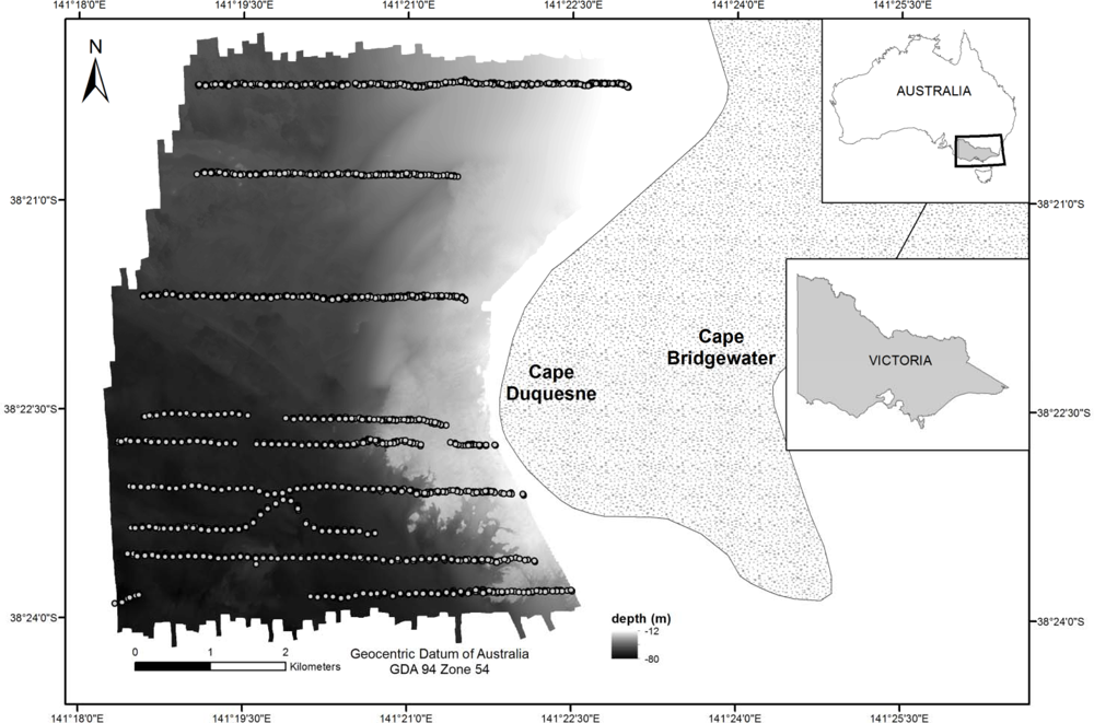
The study area is located on the western side of Cape Duquesne in Discovery Bay, south-eastern Australia. Depth ranged from 12 m to 80 m (Figure 1). The shallow reef structures supported diverse assemblages of red algae and kelps, dominated by Ecklonia radiata, Phyllospora comosa and Durvillaea potatorum. Deeper regions were dominated by sponges, ascidians, bryozoans and gorgonian corals [15].
2.2. Acoustic Data
Acoustic data was acquired on the 6 and 7 of November 2005. The acquisition system consisted of a hull-mounted Reson Seabat 8,101 MBES. The Seabat 8,101 operated at a frequency of 240 kHz, designed specifically for shallow water surveying purposes. This swath system consisted of 101 individual beams and each with a beamwidth of 1.5° (along and across track). Horizontal positioning was accomplished using Starfix HP Differential GPS system (±0.30 m) integrated with a POS MV (Positioning and Orientating System for Marine Vessels) for heave, pitch, roll and yaw corrections (±0.02° accuracy). Real-time navigation, data-logging, quality control and display were made possible using the Starfix suite 7.1 software (Fugro Survey Pty Ltd.). Daily sound velocity profiles were collected to correct for water column sound speed variations. For backscatter data, raw amplitudes were post processed using the Centre for Marine and Technology’s (CMST) software [10] to generate a backscatter image and to extract angular backscatter intensity. The CMST software applied geometric and radiometric corrections. Geometric corrections included vessel movement (e.g., roll, pitch, yaw, heave and heading) and slant range to estimate the actual depth and location of measurements made by each beam on every ping. Radiometric correction compensated for time variable gain, spreading and absorption losses, footprint size and also angular dependence corrections. Angular dependence correction used a ‘sliding window’ every 25 consecutive pings to obtain normalised backscatter using a reference angle of 30°. A spatial interpolation Kriging method was then applied to produce a backscatter image with 5 m pixels. In addition to the backscatter image, angular intensity data was also extracted (i.e., number of pings were similar as in the angular dependence correction). Each angular backscatter curve was derived at the resolution of half a swath width, separately for port and starboard sides, located at the midpoint of each swath.
2.3. Ground Truth Data
A georeferenced towed underwater video system (Pro 3 VideoRay Remotely Operated Vehicle) was used to provide ground truth information for model building and evaluation. Underwater acoustic positioning of the towed video system was achieved using a Tracklink Ultra Short Base Line (USBL) acoustic tracking system, with vessel errors (roll, pitch and yaw) corrected using a KVH motion sensor (KVH Industries, Inc.). Wide area Differential Global Positioning System (DGPS) (OmniSTAR) was used to fix the vessel location and apply corrections for the acoustically positioned video (±2.5 m accuracy). The recorded video data was then classified according to the Victorian Towed Video Classification scheme to identify the benthic biota and substrata classes. The classification scheme followed the guidelines published by the Interim Marine and Coastal Regionalisation for Australia [16]. Biota classes were categorized into five dominant groups; Mixed Brown algae (MB), Invertebrates (INV), Mixed Red algae and Invertebrates (MRI), No Visible Biota (NVB) and Mixed Brown algae and Invertebrates (MBI). The substratum classes were Reef, Sediment and Reef/Sediment. To assign ground truth classes to angular backscatter data (i.e., for classification process) an approximate intersection method was applied by searching for the nearest majority class within a 10 m radius of the angular backscatter response location. The spatial position of the 10 m radius for the angular response was chosen by considering all swath lengths at different depths and 50% overlap of survey lines. Radii were drawn and visually checked to ensure they were not too sparse or overlapping each other. Smaller and larger radii were also tested but found to be inconsistent with the neighborhood classes. All available reference data (i.e., angular backscatter response with class name) were randomly sampled for model development (70%) and for accuracy assessment (30%).
2.4. Supervised Learning
Four supervised learning methods were used in this study to classify the angular backscatter intensity; Maximum Likelihood Classifiers (MLC), Quick Unbiased Efficient Statistical Tree (QUEST) decision tree, Random Forest (RF) decision tree and the Support Vector Machine (SVM). These supervised learning methods were used to combine ground truth data and angular backscatter response to predict habitat classes for the remaining angular backscatter data. We used 71 variables, each representing angular backscatter intensity strength at one degree incidence angle from 0° to 70°.
The MLC is a well-known parametric supervised classification approach that has been widely used in remote sensing applications [17] and produces promising results [18]. The MLC approach computes mean and covariance matrices for each class from training data and assumes that the probability density function is a normal Gaussian distribution. For classification, probability of each class is estimated from the training data and the unknown sample data is classified to the class that has the highest membership probability. We applied MLC using the Bayesian decision rule algorithms described in Theodoridis and Koutroumbas [19]. In terms of angular backscatter response classification, Simons and Snellen [4] used the Gaussian rule for designing a Bayesian classification approach, however they used averaged backscatter at a single angle while our approach utilized backscatter at various angles.
A decision tree recursively partitions a dataset into smaller subdivisions on the basis of a set of tests defined at a branch or node in the tree [20]. We applied the QUEST decision tree which has advantages over common decision tree methods such as Classification and Regression Trees (CART) by reducing the potential for over fitting [21]. The QUEST method achieves this by not employing an exhaustive variable search routine and is unbiased in choosing variables which afford more splits [22]. We used the QUEST executable program obtained from http://www.stat.wisc.edu/~loh/quest.html. We also tested a multiple decision tree approach in Random Forests (RF). The RF uses a combination of tree predictors such that each tree depends on the values of a random vector sampled independently and with the same distribution for all trees in the forest [23]. The RF generates multiple trees at each node with classes being predicted by a majority vote. Standard decision trees split each node using the best split among all variables but RF split each node using the best among a subset of predictors randomly chosen at that node. We applied RF using a function in Matlab®[24] which can be downloaded at http://code.google.com/p/randomforest-matlab/.
Support Vector Machine (SVM) is a non-parametric technique developed from statistical learning theory [25]. In SVM, a line is determined and drawn between two classes using the available training data. In a high dimensional space, this line is called a hyper plane and since many lines may occur, SVM searches for the optimal hyper plane. A radial basis kernel was applied [26] and classification run using the LIBSVM tool [27] available at http://www.csie.ntu.edu.tw/~cjlin/libsvm.
2.5. Spatial Segmentation and Class Assignment
For generation of habitat maps utilizing previous classification results from angular response curves, a spatial segmentation was applied to backscatter image. This technique segments the backscatter image into clusters of similar backscatter values. In terms of benthic habitat classification and mapping, the concept of spatial segmentation of backscatter imagery has been previously applied to assist with object image analysis and classifications [28]. For this purpose we employed a mean shift image segmentation technique available from the Edge Detection and Image Segmentation System (EDISON) tool [29]. The EDISON tool uses kernel density estimation to group pixels in feature space. The number of features included lattice coordinates (X and Y) and color layers (e.g., greyscale or color image). Since EDISON is optimized and originally developed for color image applications, we first converted the backscatter image into a pseudo color image across the RGB (Red, Green and Blue) spectrum in Matlab. Then, spatial segmentation was accomplished using default spatial and color resolutions (i.e., 7 and 6.5 respectively), with a minimum size region of 100 pixels. All the segments produced from this process were then spatially compared with angular backscatter response classification results (geographical location and predicted class) for class assignment. Because the size of each segment was different and had an irregular shape according to the original backscatter image texture, the number of angular responses in each segment was not the same. Class assignment for all segments was completed using k-nearest neighbor method (k = 7). In this process, a centroid was computed for each segment and a search was made around each centroid for the nearest angular backscatter class location. Segment maps with class labels were then converted to raster for further accuracy assessment and map comparison analysis. Application of spatial image segmentation and k-nearest neighbor for producing maps with angular response data have been described in Che-Hasan et al.[5].
2.6. Accuracy Assessment and Habitat Map Comparison
Error matrices were used to assess map accuracy utilizing 30% of ground truth observations that were not used in the classification process. For each map overall accuracy and kappa coefficient were calculated. The user and producer accuracy was also calculated to investigate individual class accuracy [30]. Kappa coefficient is the agreement between classification and reference data and to correct for chance agreement between classes [31]. User’s accuracy indicates the probability that the actual map pixel represents the category on the ground, while producer’s accuracy is the probability of a reference pixel being correctly classified [32]. A Z statistic was applied to determine the differences in classification accuracy for the four methods [30]. To critically evaluate the spatial distribution of predicted habitat using the different techniques, we performed map comparison analysis using the Map Comparison Kit[33]. Similarity between any two categorical maps was assessed in terms of Kappa Location (KLoc) and Kappa Histogram (KHisto) statistics. KLoc represents the similarity of spatial allocation of categories between two maps, while KHisto is a measure for the quantitative similarity (i.e., quantity in terms of fraction of all cells) [33].
2.7. Variable Importance Measure
At each bootstrap iteration of the RF process the resultant tree is used to predict those data not included in the training process (‘out of bag’ or OOB observations) and calculate a misclassification rate [23,34]. An advantage of using RF ensemble methods over a single classification tree approach is that OOB samples for each tree can then be used to derive measures of variable importance. The importance of a given feature is evaluated based on the difference between the misclassification rate of the OOB data and the misclassification rate if values of a given variable are randomly permuted for the OOB observations and passed down the tree to create new predictions. RF can produce not only overall, but also per class variable importance. For comparison purposes, variable importance values were scaled from 0 to 1 as classes exhibited differing ranges.
3. Results
3.1. Habitat Map Accuracy
The overall accuracy varied from 69.9% to 84.8% for the biota classifications (Table 1). The highest accuracy was achieved by SVM, presented in Figure 2. This was then followed by RF, QUEST and MLC. Statistical comparison of error matrices using the four techniques revealed that QUEST, RF and SVM were significantly different from the MLC approach (Z > 1.96; Table 2). The QUEST, RF and SVM produced similar results, except for the comparison of QUEST and SVM which was significantly different (Z = 2.2).
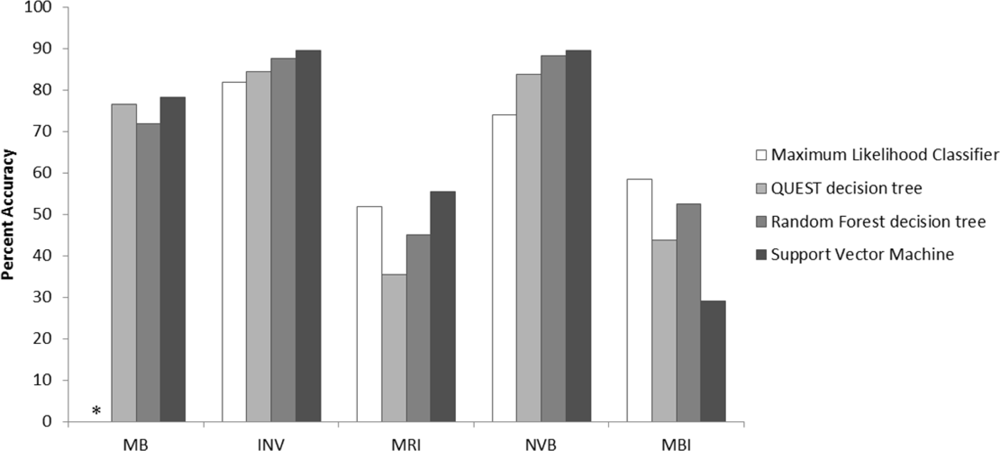
Per class accuracy measurement (average of user’s and producer’s accuracy) illustrated that most of the classes were able to be distinguished, except for the MLC which was not able to differentiate the MB class (0%) (Figure 3). Generally, MB, INV and NVB showed >70% accuracy while MRI and MBI showed lowest class accuracy (<60%).
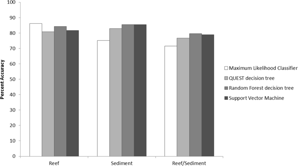
Characterizing substratum types using the same classifiers exhibited similar results as the biota classifications (Table 1). The RF (83.0%; Figure 2) and SVM (82.6%) performed best, followed by QUEST (80.2%) and MLC (74.5%). A pairwise comparison from all non-parametric classifiers (QUEST, RF and SVM) demonstrated that their results were not significantly different (Z < 1.96) except with MLC (Table 2). Individual accuracy from all three substratum classes showed values >70% from all classifiers with MLC achieving the highest accuracy for reef class (86.1%) (Figure 4).
3.2. Habitat Map Comparison
In general, all biota habitat maps showed considerable agreement in terms of the spatial location (KLoc from 0.70 to 0.90) and quantity (KHisto from 0.75 to 0.98) (Table 3). However, no single classifier combination gained both the highest KLoc and KHisto. For KLoc, the comparison between RF and SVM showed the highest similarity (0.90). For KHisto, the highest similarity was achieved between QUEST and SVM (0.98). All the comparisons with the MLC map yielded the lowest map similarity values.
For substratum habitat map comparisons all map comparisons produced good KHisto values ranging from 0.83 to 0.97. Further, the QUEST, RF and MLC represent the highest map similarity with KHisto of 0.97 (QUEST and RF) and 0.95 (MLC and QUEST, MLC and RF). The RF and SVM revealed the highest similarity of spatial location (KLoc = 0.94).
3.3. Variable Importance
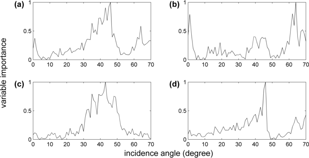
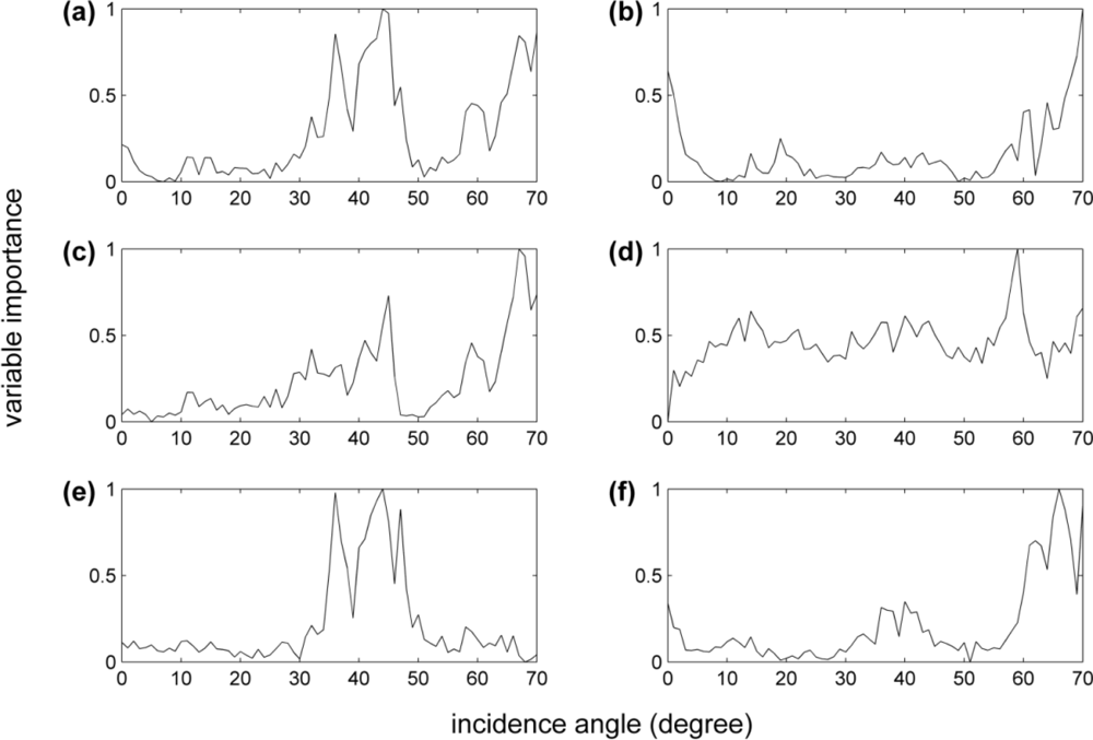
The variables at the moderate incidence angle (i.e., 30°–50°) were generally found to be the most important (Figures 5 and 6). Some variables at the outer angle were also important especially for biota (Figure 5(a)), but slightly lower for substratum (Figure 6(a)). However, the variable importance for the individual habitat classes showed a slightly different trend when compared to the overall variable importance (Figure 5(b–f)). Variables at the outer angle were identified as important for MB, MBI and INV. The moderate incidence angle was the most important variable for NVB. Further, there was not a clear pattern of which angular domain was important for MRI. Although variable importance for MRI shows highest value at incidence angle around 60°, it was only from a single variable. A similar pattern was observed for substratum classes (Figure 6(b–d)). Most of the variables at the moderate incidence angle were important for Sediment. By contrast, only small numbers of variables at the outer and near nadir angles were important for Reef/Sediment.
4. Discussion
In this study we have applied four supervised learning methods to classify the angular response from MBES data to distinguish biotic and substratum habitats. Generally, all classifiers were capable of using angular backscatter data for predicting different habitat types, with SVM (biota) and RF (substratum) achieving the highest accuracy. The application of automated classifiers using angular response data are becoming more common [4,8]. The results of our study permit a direct comparison of classifier performance, as the same training and test data were applied for all four supervised learning methods. In addition, our approach identified the most influential angular domain that contributed to the differentiation of habitat classes, which is often difficult to quantify from acoustic scattering properties.
Classification comparisons suggested that the three non-parametric classifiers (SVM, RF and QUEST) mostly performed better compared to the parametric method (MLC) for classifying biotic habitat classes. Although MLC is a standard and widely used approach for classification of satellite imagery, the disadvantage of a parametric method is that a Gaussian frequency distribution is assumed in feature space for each class. Normal distribution (i.e., Gaussian) has been applied with angular backscatter response data using a Bayesian classification approach at a single angle [4]. This method was found to be useful for construction of generic acoustic models at near nadir angle [3]. However, the distribution of backscatter can differ between angular regimes and seafloor types; as such it may not be appropriate to assume the same distribution for all incidence angles [35]. Among the four classifiers, MLC uses the simplest method of discrimination using the mean and standard deviation between each class. This study demonstrated that these values may not be appropriate for angular response backscatter classification; especially for habitats that share similar characteristics with small class separation (i.e., MB and MBI). By contrast, decision tree methods and SVM implement more advanced rules to separate between classes. For example, a decision tree approach is capable of constructing hundreds of decision rules. Similarly, a SVM approach generates complex multidimensional lines dependent on the kernel function employed. Nevertheless, in terms of overall kappa analysis, MLC accuracy performs similar to SVM with a moderate classification agreement (i.e., Kappa coefficient between 0.40 and 0.80) [36].
RF, QUEST and MLC classification of substratum was slightly better or more consistent than the biota classifications. The SVM approach is sensitive to parameter values especially choice of kernels, regularization parameter and kernel width [27]. In reviews of SVM application in terrestrial remote sensing, studies have identified this issue as one of its limitations [37]. Accordingly, SVM needs correct parameter calibration to get consistent results with the two classification schemes (i.e., biota and substratum classifications), potentially requiring different values for these parameters. However, there is no heuristic method to obtain correct parameters necessitating a trial-and-error approach [37]. The common approach of parameter calibration or selection in SVM is to run multiple SVM classifications using a range of values for each parameter [27]. The best value is determined by the highest accuracy of the SVM internal cross validation process within the training data. This approach is not practical for application in this study, because our thematic map accuracy assessment was based on the spatial location of angular backscatter response (30% training data), and not using the original variables (i.e., the angular backscatter response data) [36].
The comparison between two categorical maps is commonly applied in terrestrial applications, and is becoming increasingly important for applications in benthic habitat mapping [38–40]. In this study, map comparison did not identify the most accurate classifier; rather it measured the relative agreement between two thematic maps. Therefore, the similarity analysis produced in this study is a representation of precision, not a level of accuracy. The results of this analysis complement the information provided by the accuracy assessment and Z-statistic test, which was based on an error matrix. Values of KLoc and KHisto showed moderate agreement between the classification map sets presented. The relatively moderate agreement observed could be explained as a function of the small number of classes involved. The relatively large areas of some of the classes may also result in over estimation of map similarity measures. For example, INV and NVB (biota map) and Reef and Sediment (substratum map) dominated approximately 80% of the study site. Measures of similarity between map comparisons may also be a function of the same segmentation and class assignment process applied for each classifier used to increase the spatial resolution of classification outputs.
For classifications of biota and substratum, the variables at the moderate incidence angle were the most important. This is in agreement with previous studies [7,8,10]. Hamilton and Parnum [8] showed that angular backscatter response from 35° to 45° exhibited large class separation. They also suggested that the near nadir angles (±15° to 20°) may be less useful in the classification process. A similar pattern was also observed for angular response curves from soft-smooth and hard-rough habitats [7]. Nevertheless, the near nadir and outer angles may provide useful information for class separation and are used for Angular Range Analysis (ARA) to predict sediment types [1]. This was evident from different patterns in the variable importance measure from each habitat class. The moderate incidence angles were useful in distinguishing NVB from the remaining biotic habitats. However, other angles were necessary to separate INV, MRI, MB and MBI classes. The importance of the outer angles identified in this study may be confounded by local variation in bathymetry (slope, bedforms) or the MBES data collection approach (shore parallel) which may influence the angular response at the outer angles by the localized gradient in the study area. This could potentially explain the more complex angular response curves observed in classes with expected high topographic complexity. Future work may evaluate response curves for classes found on topographically variable terrain (i.e., macro algae on flat pavement vs. high profile rugose reef). Furthermore, peaks in incidence angles greater than 60° may also be caused by the changeover of different backscatter detection methods during data acquisition (amplitude detection at inner beams towards phase detection on the outer beams) [41].
The application of classifiers at a single angle is useful for discriminating sediment types [4]. However there may be advantages in taking into account multiple angles within a single classification process. The inclusion of more variables representing incident angles could potentially result in a better model fit, and greater separability of classes by using the entire backscatter angular response.
This study extends the approach presented by Rzhanov et al.[14] combining the angular response analysis with information from the segmented backscatter image for characterizing biota habitats. An angular based approach takes advantage of the variation in acoustic response between habitat variables defined across the entire angular range. Concurrently, an image-based approach takes advantage of the spatial resolution afforded by using image based segmentation. There are some considerations that need to be taken into account when combining angular and image datasets. For example, the angular response derived from port or starboard may not necessarily represent homogenous regions in backscatter image intensity, thus containing multiple segments. In the case of angular response derived from a homogenous segment, only a partial rather than a full response curve is used in the classification process for class assignment. In these situations it is likely that there will be more difficulty in the classification process because the use of information from a partial response curve may reduce class separability. Whilst an image segmentation approach was employed for class assignment, the methodology does not take advantage of the spatial variability in the backscatter image during the actual classification process. Rather than using a classification approach to combine angular response class assignment outputs to an image, an alternative approach may be to assign angular response parameterization values to image segments that could be combined with additional data sources during the classification process. For example, the differentiation of substratum and biota classes may be improved by incorporating bathymetry and derivatives [42,43], backscatter textural analysis [44] and other environmental variables such as exposure [45].
5. Conclusions
In this study four supervised learning approaches were evaluated for acoustic characterization of seafloor habitats using multibeam echo-sounder backscatter data. To construct a full coverage habitat map, classified angular response data were combined using a backscatter image segmentation process. It was possible to achieve overall classification accuracies between 69.9% to 84.8% (kappa values of 0.51–0.75) for biota and 74.5% to 83% (kappa values of 0.59–0.71) for substratum maps. SVM performed best for biota (84.8%, kappa = 0.75) and RF produced best results for substratum (83%, kappa = 0.72) with no significant difference between classifier performance. QUEST achieved lower accuracies than RF for biota and substrata (79.6% and 80.2% respectively) and significantly lower accuracies than SVM for biota (79.6%). MLC achieved better overall accuracies for substratum than biota (74.5% and 69.9% respectively), however, results were significantly lower than the other classifiers tested. Maps produced from all classifiers were showing moderate to good similarities in terms of pixel quantity (KHisto from 0.75 to 0.98) and location (KLoc from 0.69 to 0.94). The small number of classes and relatively large areas may contribute to the high map similarity measures observed. This study also quantifies the relative importance of angular domains, with moderate incidence angles (30°–50°) contributing most to the class differentiation process. The near nadir angles (0°–30°) and outer angles (60°–70°) also showed small contributions to class discrimination however the influence of local depth gradient and slope warrants further investigation. The approach presented has the advantage of class discrimination using the full angular backscatter response in conjunction with the spatial resolution achieved by integrating an image segmentation method.
Acknowledgments
This work was supported by the National Heritage Trust and Caring for our Country as part of the Victorian Marine Habitat Mapping Project with project partners Glenelg Hopkins Catchment Management Authority, Department of Sustainability and Environment, Parks Victoria, University of Western Australia and Fugro Survey. Thanks to crew from the Australian Maritime College research vessel Bluefin used for the multibeam data collection. Thanks also to P.J.W. Siwabessy (Geoscience Australia) for modification of CMST software and R.G. Congalton for the Kappa program. This paper has been greatly improved by comments from five anonymous reviewers.
References
- Fonseca, L.; Mayer, L. Remote estimation of surficial seafloor properties through the application Angular Range Analysis to multibeam sonar data. Mar. Geophys. Res 2007, 28, 119–126. [Google Scholar]
- Hughes-Clarke, J.E.; Danforth, B.W.; Valentine, P. Areal Seabed Classification using Backscatter Angular Response at 95 kHz. High Frequency Acoustics in Shallow Water (NATO SACLANTCEN Conference Proceedings), Series CP-45; Pace, N.G., Pouliquen, E., Bergem, O., Lyons, A.P., Eds.; Office of Naval Research, United States National Liaison Officer to the SACLANTCEN: Arlington, VA, USA, 1997; pp. 243–250. [Google Scholar]
- Lamarche, G.; Lurton, X.; Verdier, A.-L.; Augustin, J.-M. Quantitative characterization of seafloor substrate and bedforms using advanced processing of multibeam backscatter—Application to Cook Strait, New Zealand. Cont. Shelf Res 2010, 31, S93–S109. [Google Scholar]
- Simons, D.G.; Snellen, M. A Bayesian approach to seafloor classification using multi-beam echo-sounder backscatter data. Appl. Acoust 2009, 70, 1258–1268. [Google Scholar]
- Che-Hasan, R.; Ierodiaconou, D.; Laurenson, L. Combining angular response classification and backscatter imagery segmentation for benthic biological habitat mapping. Estuar. Coast. Shelf Sci 2012, 97, 1–9. [Google Scholar] [Green Version]
- De Falco, G.; Tonielli, R.; Di Martino, G.; Innangi, S.; Simeone, S.; Parnum, I.M. Relationships between multibeam backscatter, sediment grain size and Posidonia oceanica seagrass distribution. Cont. Shelf Res 2010, 30, 1941–1950. [Google Scholar]
- Kloser, R.J.; Penrose, J.D.; Butler, A.J. Multi-beam backscatter measurements used to infer seabed habitats. Cont. Shelf Res 2010, 30, 1772–1782. [Google Scholar]
- Hamilton, L.J.; Parnum, I. Acoustic seabed segmentation from direct statistical clustering of entire multibeam sonar backscatter curves. Cont. Shelf Res 2011, 31, 138–148. [Google Scholar]
- Parnum, I.M.; Gavrilov, A.N. High-frequency multibeam echo-sounder measurements of seafloor backscatter in shallow water: Part 2 Mosaic production, analysis and classification. Underwater Technology 2011, 30, 13–26. [Google Scholar]
- Parnum, I.M. Benthic Habitat Mapping Using Multibeam Sonar Systems. Curtin University of Technology, Bentley, WA, Australia, 2007. [Google Scholar]
- Jackson, D.R.; Winebrenner, D.P.; Ishimaru, A. Application of the composite roughness model to high-frequency bottom backscattering. J. Acoust. Soc. Am 1986, 79, 1410–1422. [Google Scholar]
- Augustin, J.M.; Suave, R.; Lurton, X.; Voisset, M.; Dugelay, S.; Satra, C. Contribution of the multibeam acoustic imagery to the exploration of the sea-bottom. Mar. Geophys. Res 1996, 18, 459–486. [Google Scholar]
- Fonseca, L.; Brown, C.; Calder, B.; Mayer, L.; Rzhanov, Y. Angular range analysis of acoustic themes from Stanton Banks Ireland: A link between visual interpretation and multibeam echosounder angular signatures. Appl. Acoust 2009, 70, 1298–1304. [Google Scholar]
- Rzhanov, Y.; Fonseca, L.; Mayer, L. Construction of seafloor thematic maps from multibeam acoustic backscatter angular response data. Comput. Geosci 2012, 41, 181–187. [Google Scholar]
- Ierodiaconou, D.; Rattray, A.; Laurenson, L.; Monk, J.; Lind, P. Victorian Marine Habitat Mapping Project; Deakin University: Geelong, VIC, Australia, 2007. [Google Scholar]
- The Interim Marine and Coastal Regionalisation for Australia: An Ecosystem-Based Classification for Marine and Coastal Environments (Version 3.3); Environment Australia-Commonwealth Department of the Environment: Canberra, ACT, Australia, 1998.
- Manandhar, R.; Odeh, I.; Ancev, T. Improving the accuracy of land use and land cover classification of Landsat data using post-classification enhancement. Remote Sens 2009, 1, 330–344. [Google Scholar]
- Dean, A.M.; Smith, G.M. An evaluation of per-parcel land cover mapping using maximum likelihood class probabilities. Int. J. Remote Sens 2003, 24, 2905–2920. [Google Scholar]
- Theodoridis, S.; Koutroumbas, K. Classifiers Based on Bayes Decision Theory. In Pattern Recognition, 4th ed; Academic Press: Boston, MA, USA, 2009. [Google Scholar]
- Friedl, M.A.; Brodley, C.E. Decision tree classification of land cover from remotely sensed data. Remote Sens. Environ 1997, 61, 399–409. [Google Scholar]
- Gray, J.B.; Fan, G. Classification tree analysis using TARGET. Comput. Stat. Data Anal 2008, 52, 1362–1372. [Google Scholar]
- Loh, W.Y.; Shih, Y.S. Split selection methods for classification trees. Stat. Sin 1997, 7, 815–840. [Google Scholar]
- Breiman, L. Random Forests. Mach. Learn 2001, 45, 5–32. [Google Scholar]
- Jaiantilal, A. Classification and Regression by Randomforest-Matlab. 2009. Available online: http://code.google.com/p/randomforest-matlab (accessed on 12 December 2010).
- Vapnik, V.N. An overview of statistical learning theory. IEEE Trans. Neural Netw 1999, 10, 988–999. [Google Scholar]
- Kavzoglu, T.; Colkesen, I. A kernel functions analysis for support vector machines for land cover classification. Int. J. Appl. Earth Obs. Geoinf 2009, 11, 352–359. [Google Scholar]
- Chang, C.-C.; Lin, C.-J. LIBSVM: A library for support vector machines. ACM TIST 2011, 2, 2:27:21–27:27. [Google Scholar]
- Lucieer, V.; Lamarche, G. Unsupervised fuzzy classification and object-based image analysis of multibeam data to map deep water substrates, Cook Strait, New Zealand. Cont. Shelf Res 2011, 31, 1236–1247. [Google Scholar]
- Comaniciu, D.; Meer, P. Mean Shift Analysis and Applications. Proceedings of the 7th IEEE International Conference on Computer vision, Kerkyra, Greece, 20–27 September 1999; 2, pp. 1197–1203.
- Congalton, R.G. A review of assessing the accuracy of classifications of remotely sensed data. Remote Sens. Environ 1991, 37, 35–46. [Google Scholar]
- Cohen, J. A Coefficient of agreement for nominal scales. Educ. Psychol. Meas 1960, 20, 37–46. [Google Scholar]
- Jensen, J.R. Introductory Digital Image Processing: A Remote Sensing Perspective, 3rd ed; Pearson Prentice Hall: Upper Saddle River, NJ, USA, 2005. [Google Scholar]
- Hagen, A. Multi-method Assessment of Map Similarity. Proceedings of the 5th AGILE Conference on Geographic Information Science, Palma de Mallorca, Spain, 25–27 April 2002; 2003; pp. 171–182. [Google Scholar]
- Cutler, D.R.; Edwards, T.C.; Beard, K.H.; Cutler, A.; Hess, K.T.; Gibson, J.; Lawler, J.J. Random forests for classification in ecology. Ecology 2007, 88, 2783–2792. [Google Scholar]
- Siwabessy, P.J.W.; Gavrilov, A.N.; Duncan, A.J.; Parnum, I.M. Statistical Analysis of High-Frequency Multibeam Backscatter Data in Shallow Water. Proceedings of ACOUSTICS 2006, Christchurch, New Zealand, 20–22 November 2006.
- Congalton, R.G.; Green, K. Assessing the Accuracy of Remotely Sensed Data: Principles and Practices, 2nd ed; CRC Press: Boca Raton, FL, USA, 2009. [Google Scholar]
- Mountrakis, G.; Im, J.; Ogole, C. Support vector machines in remote sensing: A review. ISPRS J. Photogramm 2011, 66, 247–259. [Google Scholar]
- Schimel, A.C.G.; Healy, T.R.; Johnson, D.; Immenga, D. Quantitative experimental comparison of single-beam, sidescan, and multibeam benthic habitat maps. ICES J. Mar. Sci 2010, 67, 1766–1779. [Google Scholar]
- McGonigle, C.; Grabowski, J.H.; Brown, C.J.; Weber, T.C.; Quinn, R. Detection of deep water benthic macroalgae using image-based classification techniques on multibeam backscatter at Cashes Ledge, Gulf of Maine, USA. Estuar. Coast. Shelf Sci 2011, 91, 87–101. [Google Scholar]
- McGonigle, C.; Brown, C.J.; Quinn, R. Insonification orientation and its relevance for image-based classification of multibeam backscatter. ICES J. Mar. Sci 2010, 67, 1010–1023. [Google Scholar]
- Galway, R.S. Comparision of Target Detection Capabilities of the Reson Seabat 8101 and Reson Seabat 9001 Multibeam Sonars; Department of Geodesy and Geomatics Engineering, University of New Brunswick: Fredericton, NB, Canada, 2000. [Google Scholar]
- Ierodiaconou, D.; Burq, S.; Reston, M.; Laurenson, L. Marine benthic habitat mapping using multibeam data, georeferenced video and image classification techniques in Victoria, Australia. J. Spat. Sci 2007, 52, 93–104. [Google Scholar]
- Rattray, A.; Ierodiaconou, D.; Laurenson, L.; Burq, S.; Reston, M. Hydro-acoustic remote sensing of benthic biological communities on the shallow South East Australian continental shelf. Estuar. Coast. Shelf Sci 2009, 84, 237–245. [Google Scholar]
- Blondel, P.; Gómez Sichi, O. Textural analyses of multibeam sonar imagery from Stanton Banks, Northern Ireland continental shelf. Appl. Acoust 2009, 70, 1288–1297. [Google Scholar]
- Galparsoro, I.; Borja, Á.; Bald, J.; Liria, P.; Chust, G. Predicting suitable habitat for the European lobster (Homarus gammarus), on the Basque continental shelf (Bay of Biscay), using Ecological-Niche Factor Analysis. Ecol. Model 2009, 220, 556–567. [Google Scholar]
Figure 1.
Bathymetric map from multibeam echo sounder survey of the study area. The grey circles represent the ground truth data from georeferenced towed underwater video observations.
Figure 1.
Bathymetric map from multibeam echo sounder survey of the study area. The grey circles represent the ground truth data from georeferenced towed underwater video observations.

Figure 2.
Habitat maps of biota and substratum classifications from the best model (the Support Vector Machine for biota and the Random Forest decision tree for substratum).
Figure 2.
Habitat maps of biota and substratum classifications from the best model (the Support Vector Machine for biota and the Random Forest decision tree for substratum).
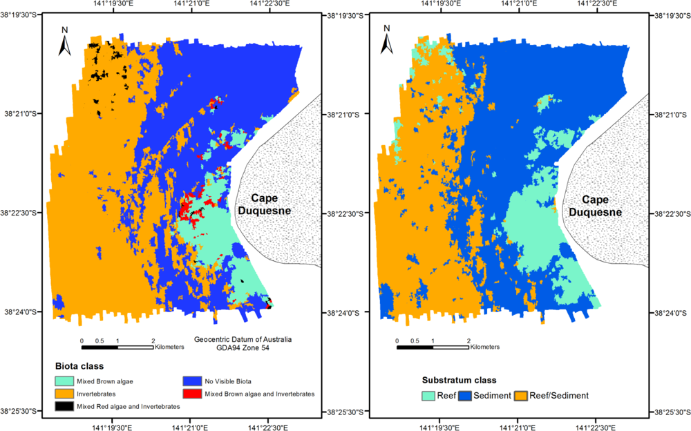
Figure 3.
Per class accuracy (mean value between user and producer’s accuracy) for five biota classes and four different classifiers. *Note that the average accuracy of MB = 0% for Maximum Likelihood Classifier. MB = Mixed Brown algae, INV = Invertebrates, MRI = Mixed Red algae and Invertebrates, NVB = No Visible Biota, MBI = Mixed Brown Invertebrates.

Figure 4.
Per class accuracy (mean value between user and producer’s accuracy) for three substratum classes and four different classifiers.
Figure 4.
Per class accuracy (mean value between user and producer’s accuracy) for three substratum classes and four different classifiers.

Figure 5.
Variable importance (overall and individual class) from Random Forest model scaled from 0 to 1 for biota classification. The horizontal axis represents incidence angle at one degree interval while the vertical axis represents the value of the variable importance. (a) Overall variable importance for biota classification, (b) variable importance for Mixed Brown algae, (c) variable importance for Invertebrates, (d) variable importance for Mixed Red algae and Invertebrates, (e) variable importance for No Visible Biota, and (f) variable importance for Mixed Brown algae and Invertebrates.

Figure 6.
Variable importance (overall and individual class) from Random Forest model scaled from 0 to 1 for substratum classification. The horizontal axis represents incidence angle at one degree interval while the vertical axis represents the value of the variable importance. (a) Overall variable importance for substratum classification, (b) variable importance for Reef, (c) variable importance for Sediment, and (d) variable importance for Reef/Sediment.

| Biota | Substratum | |||
|---|---|---|---|---|
| Classifiers | Overall Accuracy (%) | Kappa Coefficient | Overall Accuracy (%) | Kappa Coefficient |
| Maximum Likelihood Classifier | 69.9 | 0.51 | 74.5 | 0.59 |
| QUEST decision tree | 79.6 | 0.66 | 80.2 | 0.67 |
| Random Forest decision tree | 83.8 | 0.73 | 83.0 | 0.72 |
| Support Vector Machine | 84.8 | 0.75 | 82.6 | 0.71 |
Table 2.
Z values from pairwise comparison of error matrices between different classifiers. MLC = Maximum Likelihood Classifier, QUEST = QUEST decision tree, RF = Random Forest decision tree, SVM = Support Vector Machine.
| Comparison | Z Statistic | |
|---|---|---|
| Biota | Substratum | |
| MLC vs. QUEST | 3.6* | 2.0* |
| MLC vs. RF | 5.6* | 3.1* |
| MLC vs. SVM | 6.0* | 2.8* |
| QUEST vs. RF | 1.8 | 1.1 |
| QUEST vs. SVM | 2.2* | 0.8 |
| RF vs. SVM | 0.4 | 0.3 |
*Significant at the 95% confidence interval (critical value Z = 1.96).
Table 3.
Results from habitat map comparisons. KLoc = measure for the similarity of spatial allocation, KHisto = measure for the quantitative similarity. MLC = Maximum Likelihood Classifier, QUEST = QUEST decision tree, RF = Random Forest decision tree, SVM = Support Vector Machine.
| Map Comparison | Biota | Substratum | ||
|---|---|---|---|---|
| KLoc | KHisto | KLoc | KHisto | |
| MLC vs. QUEST | 0.76 | 0.75 | 0.69 | 0.95 |
| MLC vs. RF | 0.70 | 0.81 | 0.70 | 0.95 |
| MLC vs. SVM | 0.70 | 0.76 | 0.70 | 0.88 |
| QUEST vs. RF | 0.88 | 0.91 | 0.87 | 0.97 |
| QUEST vs. SVM | 0.79 | 0.98 | 0.87 | 0.83 |
| RF vs. SVM | 0.90 | 0.90 | 0.94 | 0.84 |
Share and Cite
MDPI and ACS Style
Hasan, R.C.; Ierodiaconou, D.; Monk, J. Evaluation of Four Supervised Learning Methods for Benthic Habitat Mapping Using Backscatter from Multi-Beam Sonar. Remote Sens. 2012, 4, 3427-3443. https://doi.org/10.3390/rs4113427
AMA Style
Hasan RC, Ierodiaconou D, Monk J. Evaluation of Four Supervised Learning Methods for Benthic Habitat Mapping Using Backscatter from Multi-Beam Sonar. Remote Sensing. 2012; 4(11):3427-3443. https://doi.org/10.3390/rs4113427
Chicago/Turabian StyleHasan, Rozaimi Che, Daniel Ierodiaconou, and Jacquomo Monk. 2012. "Evaluation of Four Supervised Learning Methods for Benthic Habitat Mapping Using Backscatter from Multi-Beam Sonar" Remote Sensing 4, no. 11: 3427-3443. https://doi.org/10.3390/rs4113427