A Quantitative Approach for Analyzing the Relationship between Urban Heat Islands and Land Cover


Remote Sensing Division (DSR), National Institute of Space Research (INPE), Avenida dos Astronautas, São José dos Campos-SP, 1758, Brazil
*
Author to whom correspondence should be addressed.
Remote Sens. 2012, 4(11), 3596-3618; https://doi.org/10.3390/rs4113596
Submission received: 30 September 2012
/
Revised: 12 November 2012
/
Accepted: 12 November 2012
/
Published: 20 November 2012
(This article belongs to the Special Issue Thermal Remote Sensing Applications: Present Status and Future Possibilities)
Abstract
:With more than 80% of Brazilians living in cities, urbanization has had an important impact on climatic variations. São José dos Campos is located in a region experiencing rapid urbanization, which has produced a remarkable Urban Heat Island (UHI) effect. This effect influences the climate, environment and socio-economic development on a regional scale. In this study, the brightness temperatures and land cover types from Landsat TM images of São José dos Campos from 1986, 2001 and 2010 were analyzed for the spatial distribution of changes in temperature and land cover. A quantitative approach was used to explore the relationships among temperature, land cover areas and several indices, including the Normalized Difference Vegetation Index (NDVI), Normalized Difference Water Index (NDWI) and Normalized Difference Built-up Index (NDBI). The results showed that urban and bare areas correlated positively with high temperatures. Conversely, areas covered in vegetation and water correlated positively with low temperatures. The indices showed that correlations between the NDVI and NDWI and temperature were low (<0.5); however, a moderate correlation was found between the NDBI and temperature.
1. Introduction
The urban heat island (UHI) effect has been a concern for more than 30 years in Brazil. One of the earliest UHI studies in a Brazilian urban center was conducted in the early 1980’s [1] in the São Paulo Metropolitan Region. The rapid urbanization of this region modified the energy and water balance processes that influence the dynamics of air movement [2]. Since then, UHI effects have been the focus of study of sciences related to geography, urban areas and human health. The UHI effect has been detected in the city center of Shanghai, China. Mortality rates related to heat waves have been higher in urban areas compared to suburban areas because the UHI effect enhances the intensity of heat waves, which exposes the local populations to extreme thermal conditions [3].
The highest correlation between UHIs and air pollution in São Paulo Metropolitan Region occurs in the austral winter [1]. UHI’s intensity was found to be inversely associated with the rural temperature. Tarifa [4] studied the urban area of São José dos Campos and observed differences in air temperature and humidity between rural and urban areas of 3.4 °C and 12%, respectively. According to Lombardo [1], the spatial extent of UHIs was dependent on economic factors, with poor, industrial and densely populated areas of the São Paulo Metropolitan Region showing the most intense UHI effects. Lombardo also observed that during weekends, UHI effects decreased and the concentration of pollutants and the volume of precipitation changed. This effect was also observed by Ashworth [5] in Rochdale, USA.
As observed by Chandler [6] and Lombardo [1], UHIs can be attributed to three factors: (1) the effects of energy transformation in cities; (2) the decrease of evapotranspiration; and (3) the production of anthropogenic energy. According to Voogt [7], there are three types of UHIs: (1) Canopy Layer Heat Island (CLHI); (2) Boundary Layer Heat Island (BLHI); and (3) Surface Heat Island (SHI). Fabrizi et al.[8] described the difference between the types of UHI, characterizing the CLHI and BLHI as warming the urban atmosphere and the SHI as warming the urban surface. The main difference between the CLHI and SHI is the location where the temperature is detected. The CLHI is typically detected by ground stations using thermometers to measure air temperature in the canopy layer, while thermal remote sensors observe the spatial patterns of upwelling thermal radiance to estimate the land surface temperatures (LST) [9,10] of the SHI.
The use of thermal remote sensing data was first demonstrated by Rao [11]. Rao identified urban areas by analyzing satellite thermal infrared data. Lombardo [1] proposed a computational model for studying satellite thermal images of the São Paulo Metropolitan Region’s UHI using LST measurements. Lombardo’s analysis [1] was conducted using NOAA-7 data for regional-scale urban temperatures. Recent studies have used the Landsat Thematic Mapper (TM) and Enhanced Thematic Mapper Plus (ETM+) thermal infrared (TIR) data with 120 m and 60 m spatial resolutions, respectively, for local-scale analysis of the UHI in Brazilian urban areas [12].
Studies have shown a relationship between UHIs and patterns of land cover changes, with many indicating that the presence of vegetation and water lessened the intensity of UHIs while increased urbanization intensified the effect. However, these changes in the land cover patterns were analyzed qualitatively according to their relationship with the LST. To quantify these changes, normalized indices such as the Normalized Difference Vegetation Index (NDVI), Normalized Difference Water Index (NDWI) and Normalized Difference Built-up Index (NDBI) have been used to represent land cover changes [13,14]. Thus, the relationship between different indices and temperature can be established in UHI studies.
The purpose of our study was to quantitatively examine changes in land cover patterns and to investigate and quantify the impact of such changes on the intensity and spatial patterns of SHIs. A hybrid-supervised classification was used to extract land cover information from remote sensing images of the urban areas of São José dos Campos for different time periods. In addition, LSTs retrieved from the thermal infrared band were analyzed and the NDVI, NDWI and NDBI indices were used to quantify the land cover changes for the analyzed period.
2. Data and Methods
2.1. Study Area and Data
São José dos Campos (SJC), which is located between 22°47′–23°40′W and 46°11′–45°16′S (Figure 1) in eastern São Paulo State, Brazil, was selected as the study area because of its rapid urbanization over the past 30 years [15] and intense transformations over the last century. Industrial growth and increases in technological production and specialized services have modified the environment and climate of SJC, which is now a major industrial center in São Paulo State.
To quantitatively measure the SHI effect and classify the land cover patterns in the study area, only cloudless Landsat 5 TM images were used from 6 August 1986, 15 August 2001, and 24 August 2010. All bands from the images were applied in our analysis. The bands 1–5 and 7 have a spatial resolution of 30 m, and the thermal infrared band (band 6) has a spatial resolution of 120 m.
2.2. Image Processing
The images used were georeferenced and acquired from the United States Geological Survey (USGS) database. They were processed using the following software: Environment for Visualizing Images (ENVI) 4.8 (ITT Visual Solutions, Boulder, CO, USA), Georeferenced Information Processing System (SPRING) 5.2 [16] and ArcGIS Desktop 10 (ESRI, Redlands, CA, USA).
2.2.1. Derivation of Brightness Temperature
The sensor TM band 6 on Landsat 5 measures the radiances at the top of the atmosphere, and its brightness temperatures can be derived using Plank’s law [17]. Because the wavelengths of thermal infrared (TIR) are usually long (>10 μm), scattering and absorption are low. However, Landsat TM 5 showed only one band in the TIR spectral region. Cristóbal et al.[18] discussed using atmospheric correction of Landsat TM TIR bands by comparing them with other sensors which have two or more TIR bands and indicated the need for correction by atmospheric radiosoundings. However, as discussed in their paper, a single atmospheric radiosounding did not provide a representative value for the atmospheric conditions of the entire area covered by a Landsat image (approximately 180 × 185 km2). Jiménez-Muñoz and Sobrino [19] created a water vapor dependent model, but the authors [18] assumed that for water vapor contents higher than 3 g·cm−2, the single-channel algorithm was not accurate and should not be applied. Because of these uncertainties, we did not consider the influence of atmosphere on radiance temperature.
The at-satellite brightness temperature was used to infer the distribution of LSTs. Images from August (winter period) were used for each analyzed year, which allowed for comparison of temperature between the images. Water vapor content is also relatively low during the winter period. Thus, the UHI effect can be measured for the individual thermal images and across different time periods.
The retrieval method of brightness temperature from band 6 of the TM5 images was chosen after an analysis between two methods proposed by Chen et al.[20] and Sobrino et al.[21]. The results of each method were compared to in situ data from three meteorological stations of the Brazilian National Institute of Meteorology (INMET). The most positively correlated temperature was obtained using the method proposed by Chen et al.[20], which infers the radiance from the raw satellite image and converts the spectral radiance to temperature.
Following the method of Chen et al.[20], conversion of the digital numbers (DNs) from band 6 to spectral luminance (mW·cm−2·sr−1) was estimated by the following equation:
where DN represents the digital number of band 6; RMAX = 1.896 (mW·cm−2·sr−1); and RMIN = 0.1534 (mW·cm−2·sr−1).
The conversion from spectral radiance to temperature in °C was realized using Equation (2):
where K1 = 1,260.56 and K2 = 60.766 (mW·cm−2·sr−1·μm) are constants from a pre-launch calibration and b = 1.239 (μm) is the effective spectral range when the sensor’s response is higher than 50%.
2.2.2. Derivation of Normalized Indices
The normalized indices NDVI [22], NDWI [23] and NDBI [24] were used to characterize the land cover types and quantify the relationships between land cover type and UHI effect. To estimate NDVI and NDWI, we used the surface reflectances of the required bands used for their equation. The radiometric calibration was achieved by the equations and rescaling factors proposed by Chander et al.[25]. An atmospheric correction was performed using MODTRAN4 implemented in ENVI FLAASH [26] to retrieve surface reflectances.
NDVI (Equation (3)) is widely used because of its advantages, such as lower influence of atmospheric variations, greater sensitivity to chlorophyll, the reduction of noise by normalization between −1 and +1 and the possibility to monitor seasonal changes. However, this index also shows deficiencies, such as sensitivity to noisy additive effects, high sensitivity to variations of the canopy and substrate saturation when the leaf area index is very high, which makes it insensitive to variations in biomass [27].
To derive the NDVI from TM/Landsat 5 images, we used the following equation:
NDWI (Equation (5)) is the Normalized Difference Water Index, which is also called the leaf area water-absent index. This index estimates the water content within vegetation [23]. According to Gao [23], this index is a measure of the liquid water molecules in vegetation that interact with solar radiation. The NDWI has been widely used because it is less sensitive to atmospheric scattering effects compared with the NDVI. However, similar to the NDVI, the NDWI did not completely remove the soil background reflectance effects.
Using TM/Landsat 5 bands, equation 6 estimated the NDWI. We used band 5 (1.65 μm) as an approximation of 1.24 μm [23]. This procedure was previously described [28–30].
According to DeAlwis et al.[31], the TM 5 band 4 was used in the NDWI estimation of biomass. However, TM 5 band 4 can also discriminate water bodies and soil moisture from vegetation. Thus, band 5 was used to characterize the variations in biomass and moisture.
The NDBI index was developed by Zha et al.[24] to analyze increments of reflectance on TM 5 bands 4 and 5 for images of urbanized and barren land areas. The researchers also observed that vegetation had a slightly higher or lower DN value on the same bands and that the minimum and maximum DNs in band 4 are much lower than those in band 5 for the same land cover. From this discovery, they developed an index to derive urbanized areas from TM/Landsat 5 images, as described in Equation (7):
In this index, the authors used DNs from TM 5 bands 4 and 5, and the same bands were used to develop the NDWI. Although they look similar, the main difference between the two indices is the patterns highlighted from each band subtraction. These two methods of constructing indices were also used by Xiong et al.[13], Chen et al.[28] and Liu et al.[32].
2.2.3. Hybrid-Supervised Classification
An initial supervised maximum likelihood classification that used training areas derived from the interpretation of Red-Green-Blue (RGB) images from TM/Landsat 5 revealed serious problems caused by spectral confusion, with bare areas erroneously classified as urban and vice versa. The problem was solved using a hybrid-supervised/unsupervised classification that was analyzed using Geographical Information System (GIS) algorithms that produced neighborhood and matricial representations [33].
The matricial representation is produced by an algorithm implemented by the GIS software SPRING, which provides a high efficiency in the representation produced by the photo-interpreter. In this algorithm, the vector’s data corresponding to the edited polygons are obtained by converting from raster to vector format. A great advantage of this procedure, in which lines were adjusted and the data were polygonalized, is that the representation is performed in the matrix and not in the vector’s data [16].
The hybrid-supervised classification approach involved two steps: (1) a supervised maximum likelihood classification for land cover and (2) the matricial representation of the erroneous areas classified in the first step.
First, our hybrid-supervised classification approach involved the application of a maximum likelihood classifier to identify the areas. The training areas for our land cover classification from August for the years 1986, 2001 and 2010 were derived from a RGB composition. We used the indices NDBI, NDVI and NDWI to compose the RGB images because the indices enhanced the remote-sensing reflectance for each element in the image. The results showed a low level of spectral confusion between bare and urbanized areas. A focal majority filter was also used to eliminate the small, isolated areas present in the classified image. Second, the supervised classified images were edited by the matricial algorithm based on the representation produced by the photo-interpreter.
2.3. Quantitative Analysis
2.3.1. Quantitative Analysis from Hybrid-Supervised Classification
To quantify the land cover change during the study period, we extracted the size (km2) of the areas the classes of each hybrid-supervised classification. We also extracted the area sizes from the temperature slices of thermal images.
Pearson’s correlation matrix was used to describe the correlations among M variables. These variables were inferred from the area size values extracted from the classified images. The correlation matrices were processed using the R software environment for statistical computing [34]. This was done in accordance to the method described by Pearson [35]. He described the correlation matrix as a square, symmetrical M × M matrix with the (ij)th element equal to the correlation coefficient r ij between the indexes i and j. The diagonal elements (correlations of variables with themselves) are always equal to unity. The correlation factors are between −1 and 1 (0: no correlation and ±1: high correlation). A positive or negative value indicates that the two correlated parameters increase (or decrease) simultaneously.
2.3.2. Quantitative Analysis from Normalized Indices
To quantify the index values and to analyze if it was caused by the land cover change, we performed our statistical sampling using the Monte Carlo Method (MCM). The MCM, also known as statistical simulation, is defined as any method that uses sequences of random numbers to perform a simulation. This process was based on the outcome of many simulations using random numbers to obtain a probable solution. This technique provides an approximate, quick answer and a high level of accuracy; however, it is possible that accuracy is increased with additional simulations [36].
To achieve our goal, we extracted 40,102 values from the products of temperature, NDVI, NDBI and NDWI from each year of analysis. Furthermore, we estimated 10,000 times the mean value using 10,056 random values, which can be derived by Equation (8):
where, in the universe X with m points, we have the vector Y with n random points.
Quantitative analyses of land cover change significance were obtained after a graphic analysis of the probability density function, which was calculated using the mean values from the MCM analysis for each year.
Quantitative analyses of significance were also obtained using the 10,000 mean values from each year and subtracting 1986’s values from 2001’s values. We also calculated the difference between 2001 to 2010 and 1986 to 2010. If the product of these operations resulted in a value below 0, then the information obtained by the normalized indices and temperature data indicated spectral confusion and the change could not be detected. If the value was above zero, the change could be detected.
Pearson’s correlation matrix was also used to compute the correlation between the indices and temperature. We extracted from each land cover pattern (water, vegetation, bare and urban) the values of each index and LST estimation. The statistical analysis was processed using the R software environment for statistical computing [34].
3. Results and Discussions
3.1. Quantitative Relationship between Urban Heat Islands and Land Cover Changes
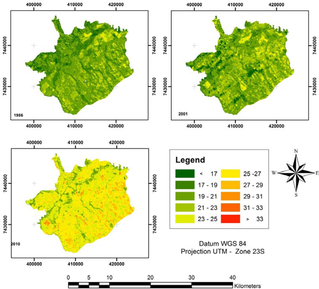
The RGB composition created by the NDVI, NDWI and NDBI was useful for identifying land cover types and allowed us to easily select training areas for the supervised maximum likelihood classification. Each composed image was ordered into 4 area classes: water, vegetation, urban and bare. Using the matricial algorithm, we could edit the urban and bare areas of high spectral confusion according to the information obtained by the photo-interpreter. The results of the classifications of land cover are found in Figure 2.
The use of indices to generate the RGB composed image was useful for identifying land cover, and in particular, the difference between urban and bare areas. Compared to the typical RGB composition using the sensor bands of each channel, the indices-generated RGB composition could discern more classes of areas. The sensitivity of the indices-generated RGB composed images arises from the purpose of the indices, which was to enhance the response of a specific target to allow for more accurate land cover interpretation.
The indices-generated RGB composition could be useful for agriculture studies because it enhances the differences in vegetation because of the NDVI and NDWI indices. The NDWI index enhances the detection of water content within vegetation, which helps eliminate the spectral confusion between bare and urban areas. This result stems from the higher water content in bare areas compared with urbanized areas. Urban areas have reduced water content because of the increased amount of impervious surfaces over the soil. However, high NDWI values could indicate high levels of air humidity, which could saturate the composed image and spoil the classification.
The visual analyses of the classifications showed an expansion in 2001 and 2010 of urban areas, which is quite noticeable when compared to the urban areas in 1986. A decrease of vegetated areas was also found for the same time period. These two facts coincided with the growth of São José dos Campos’ population. According to the Brazilian Population Census of 2010 [37], the population was 287,513 in the early 1980s, but 30 years later, the population had risen to 627,544, with 615,175 people living in urban areas.
According to Silva [38], during the period between 1980 and 2000, 421 industries were introduced to the city, which was mainly due to São José dos Campos’ strategic geographic location at the center of a route of roads connecting the 3 main southeastern States of Brazil: São Paulo, Rio de Janeiro and Minas Gerais. Beyond its geographic characteristics, the city is also attractive to the scientific community because of its technological centers, institutes and universities. The city also provides a qualified labor force for industry.
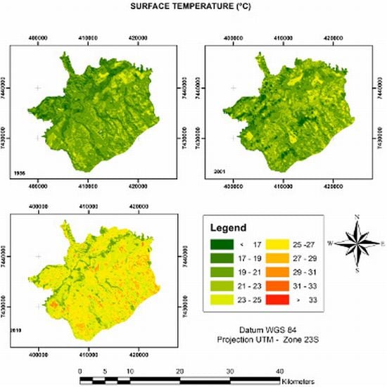
To analyze the relationship between land cover and SHIs, we extracted the LST from the TM/Landsat 5 thermal infrared band (band 6) (Figure 3). For each analyzed year, an image was produced that provided a visual resource for analyzing the intensity and spatiality of SHIs.
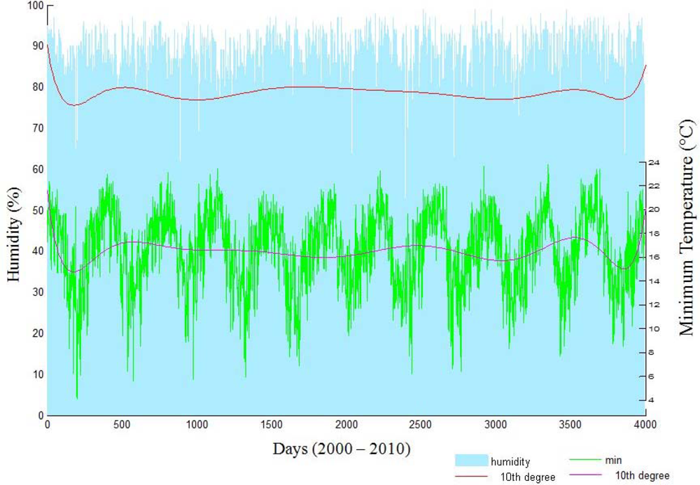
The multi-temporal analyses of LSTs showed an enormous increase in the temperature of São José dos Campos during the period from 2001 to 2010. Although the images were acquired in the same season and month, the difference in temperature was acute. This fact led us to analyze the in situ data (Figure 4) recorded at the INMET meteorological station of Mirante de São Paulo, in São Paulo.
According to the meteorological station of INMET, the temperature was 17.2 °C on 6 August 1986, 16.2 °C on 15 August 2001, and 20.4 °C on 24 August 2010. The low temperature in 2001 resulted from a La Niña climatic effect, which causes dry and cold weather in São Paulo State. These effects were easily recognized from the charts of temperature and humidity shown in Figure 4.
In Figure 4, we adjusted the minimum air temperature and mean air humidity to the period from 1 January 2000, to 31 December 2010. To easily analyze the variations, we also adjusted the curve for each parameter using a decic polynomial. The polynomial curve fitting allowed us to observe a decrease in the minimum temperature and humidity from 2000 to 2001 and 2009 to 2010 resulting from a La Niña event. However, the decreasing amplitude of the curves indicated that the lowest temperatures in the winter during the analyzed periods had increased.
The general increase of the minimum temperature over the analyzed period was most likely due to land cover changes. The size of urban and bare areas had increased, while the size of vegetated and aquatic areas had decreased. Furthermore, according to Maia et al.[39], the verticalization process within a city causes a decrease in wind speed, which promotes an increase in temperature. Thus, the urbanization process linked to the high emission of pollutants and the decrease of green areas over the last decade could be responsible for the abrupt increase in temperature.
To quantify the land cover changes and relate them to the LST changes, we quantified the classes from our hybrid classification according to temperature and land cover area (km2). The results, shown in Figure 5, were used to validate our interpretation of land cover and LST changes. The analyses of the temperature for 1986 showed that the majority of the urban areas of São José dos Campos had temperatures between 19 and 21 °C. In 2001, the temperature was transitioning between 19 and 21 °C and 21 and 23 °C. In 2010, the majority of urban areas had LSTs distributed between 23 and 25 °C and 25 and 27 °C.
To show a quantitative relationship between land cover and temperature change, we used the Pearson Correlation [35] to calculate the correlation matrix (Table 1). We used the area size data extracted from the hybrid classification for each year using the R software environment for statistical computing [34]. The highest positive correlations were found in the following ranges of temperatures: 23–25 °C, 25–27 °C, 27–29 °C, 29–31 °C and 31–33 °C. We also found the same positive correlations for temperatures <17 °C and between 21 and 23 °C. The highest negative correlations were found between the temperature range of 19–21 °C and the higher temperature ranges (23–25 °C, 25–27 °C, 27–29 °C, 29–31 °C and 31–33 °C). A high negative correlation was also found between the 19–21 °C temperature range and the size of bare areas. The highest positive correlation between land covers was found between areas of vegetation and water. The highest negative correlation was found between urban and vegetated areas.
To relate the land cover patterns to LSTs, we analyzed the correlations between the classes of land cover and LST. The best highest positive correlation was found between bare areas and temperatures between 23 °C and 33 °C. Other positive correlations were found between urban areas and temperatures above 23 °C. However, these correlations were not as high compared to what was found in bare areas.
The highest positive correlations with low temperatures were found in the classes of vegetation and water. Conversely, urban and bare areas had a high negative correlation with high temperatures.
These results showed the relationship between the land cover patterns and LST. As shown in Figure 5 and Table 1, changes in land cover patterns are highly correlated to changes in LSTs and the SHI effect.
We also found that urban and bare areas correlated positively with SHIs because the growth of urban and bare areas coincided with an increase in temperatures. Although these two land cover classes typically showed spectral confusion, the hybrid classification allowed their differentiation and showed that bare areas were most positively correlated with SHIs. Bare soil has a high reflectance intensity due to the presence of Fe2O3, sand and clay [40,41], which had a significant influence on the SHI.
3.2. Quantitative Relationship between Temperature and Index Values
Figure 3 shows the LSTs in the study area for the analyzed years, and qualitative changes in the intensity and spatial distribution of LSTs were found. However, we performed a quantitative analysis to identify independent changes in the LSTs between each year to determine if the changes were significant. The same procedure was performed to identify the significance of each index.
To show if the changes were relevant, we used the Monte Carlo Method (MCM) to simulate numerous values of mean temperature or mean index. The results were plotted in a probability density function to identify the independence of the values from each year. If the results were independent, a change would be evident.
The NDVI (Figure 6) was calculated according to Equation (4) for each image. Visual inspection ascertained the differences of each NDVI. The highest degree of difference was in 2001 (Figure 6), with a majority of NDVI values appearing to be below 0. As previously explained, in the period from June 2001 to February 2002, Brazil had experienced an atypical climatic period caused by the La Niña effect that produced very dry spring/summer seasons. During this period, most of the Brazilian States rationed electrical power because of low levels of water in hydroelectric plant reservoirs. The decreased water and dry weather were essential to the low values of the NDVI in 2001 because the index decreases as foliage comes under water stress [42]. Comparing the NDVIs of 1986 and 2010, changes were identified. The 1986 NDVI was enhanced compared to 2010; however, there were few areas in which the 1986 NDVI showed a decrease compared to 2010. This result could be explained by the maintenance provided by environmental management programs started because of concern over global natural resources.
To analyze the independence of each NDVI, a MCM was performed with the R software environment for statistical computing [34]. We calculated 10,000 times the mean value using 10,056 random points for each index. These values calculated the probability density function (PDF) (Figure 7), which allowed us to analyze if changes occurred.
In the histogram shown in Figure 7, 2001 is shown to be very atypical, with all mean values of the NDVI ranging between −0.14 and −0.12. In contrast, the majority of the NDVI mean values from 1986 and 2010 were between 0.32 and 0.34.
Although urban expansion is shown in Figure 6, the quantitative results from Figure 7 show that the mean NDVI values for 2010 are higher than for 1986. Potential explanations for the unexpected increase in vegetation were detailed by Moura et al.[43], who conducted a literature review and found that there was leaf flush at the top of the canopy, changes in leaf area index (LAI), modifications in canopy structure associated with tree mortality, diurnal variability in leaf water and clouds and aerosol effects.
The increasing concern for environmental preservation over the last decade has been influenced by environmental policy concerning global environmental changes. Thus, the size of urban green areas increased primarily because of the construction of urban parks, which have improved both environmental conservation efforts and the quality of human life.
The NDWI (Figure 8) behaved similarly to the NDVI, with most of the study area having low values in 2001 because of the hydric stress of the vegetation. In addition, 2001 also had low air humidity levels because of the La Niña effect. However, the increase of NDWI values for 2010 were caused by agricultural practices. Irrigation systems installed in agricultural areas decreased the impact of hydric stress on vegetation, and the effect was noticeable in the NDWI values north of the city. In 1986, the NDWI values were below −0.1, and in 2010, the values were approximately 0.1–0.2.
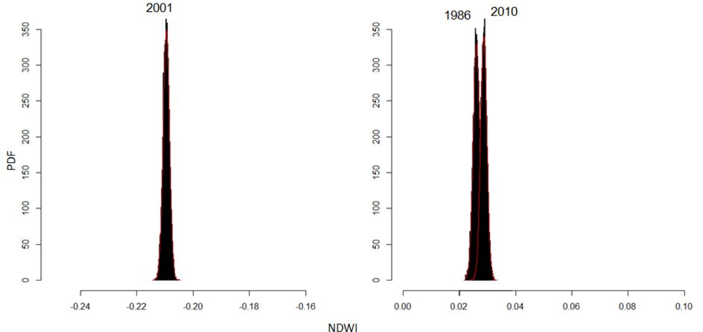
The PDF results (Figure 9) of NDWI values show low values for the 2001 NDWI, which was in the range of −0.22 to −0.20 and indicated very low air humidity and water cover and a high hydric stress for the analyzed area. When the NDWI values for 1986 and 2010 were visually overlaid, the result accounted for approximately 6% of the spectral confusion over the two year period. Out of 10,000 differences computed by the MCM, 598 were meaningless. Therefore, almost 94% of the simulated changes for the 24 years between 1986 and 2010 were significant.
The NDBI (Figure 10) for the three analyzed images were not influenced by the La Niña event in 2001 because the bands used for analysis are located on the NIR region of the electromagnetic spectrum where water content has a low influence on the processes of atmospheric absorption and scattering.
Figure 10 shows the evolution of urban expansion according to the values of the NDBI, which is shown by an increase of red areas. Analysis of the PDF results shows a quantitative discrepancy between the NDBI values between 2010 and 1986 and 2001 (Figure 11). These results show that the 2010 NDBI mean values were between 0.32 and 0.34, while in 1986 and 2001, the NDBI means values were between 0.185 and 0.195, and 0.195 and 0.21, respectively.
The results did not show any spectral confusion and the changes between years were clearly visible, demonstrating the independence and representativeness of the index. The main result of this analysis, however, was that the quantification of the NDBI could show a relationship between changes in area size and land cover class.
Therefore, the NDBI was shown to be a good estimator of urban expansion for a specific region of interest, and this finding has created new avenues of future research into UHI effects [13,28,32]. Currently, the NDBI has had difficulty differentiating between bare areas and built-up areas because of their similar reflectance in the TM/Landsat 5 bands, which is a problem that Chen et al.[28] tried to solve using the Normalized Difference Bareness Index (NDBaI).
The results of the PDF (Figure 12) for the LSTs showed a similar behavior to that of the NDBI. The main similarity was in the distribution of the mean values of temperature, which followed the chronological order of the thermal images.
As shown in Figure 12, all the mean values for the 2010 LSTs were in the range of 24.5 to 25 °C. These results were higher compared to 1986 and 2001, which were in the ranges 19.5 to 20 °C and 20 to 20.5 °C, respectively.
Finally, we compared the values from each land cover pattern with the mean yearly values for each index and LST using a correlation matrix (Tables 2–5). This procedure was performed to analyze the relationship between the indices and temperature for a specific land cover pattern.
Table 2 shows that for a water cover pattern, the values of the NDVI had a high positive correlation (r = 0.96) with the values of LST, a moderately positive correlation with the values of the NDWI and a low negative correlation with the values of the NDBI.
Table 3 shows that for a bare cover pattern, the values of the NDWI had a high positive correlation (r = 0.87) with the values of LST, a moderately positive correlation with the values of the NDVI and a low negative correlation with the values of the NDBI.
Table 4 shows that for a vegetation cover pattern, the values of the NDWI and the NDVI had a high positive correlation (r = 0.86 and 0.80) with the values of LST and a moderately negative correlation with the values of the NDBI.
Table 5 shows that for an urban land cover pattern, the values of the NDBI had a high positive correlation (r = 0.81) with the values of LST and the NDWI and the NDVI had moderately positive correlation (r = 0.46 and 0.52) with the values of LST.
The highest positive correlation was found between the NDVI and NDWI, which had an “r” of 1.00 for the urban pattern. The two indices also show a high positive correlation for the vegetation pattern (r = 0.99); however, their correlation for the water pattern was moderate (r = 0.74). It was interesting to note that in the urban pattern, the correlation between the NDVI and NDBI had an “r” of 0.92, which could be explained by the positive environmental actions promoted in the urban areas. The highest negative correlation was between the NDWI and NDBI for the water pattern, which had an “r” of −0.95.
In summary, these correlations showed the relationship between SHIs and the NDBI, and their relationship in the urban pattern has been well documented in previous studies [1,2,4,11]. However, the present study analyzed the use of indices as indicators of SHIs according to each land cover pattern. Although the correlation results between the indices and LSTs showed a moderate relationship, using indices as predictors could be an important tool for preliminary studies. New sensors from global observation programs can also improve the normalized indices within thin and specific spectral bands.
The results of the hybrid classification demonstrated that bare areas were the most positively correlated land cover pattern with SHIs. Bare areas have a high reflectance because of the soil components, as demonstrated by Price [44]. Price found that predominantly bare soil locations experienced a wider variation in LSTs. Conversely, analysis showed that the NDBI was the most positively correlated index with SHIs in an urban land cover pattern. However, it is important to note that the NDBI has a high spectral confusion rate between bare and urban areas, which could interfere with the urban pattern reflectance. The NDBI accuracy should be investigated in future studies.
The methods used in this paper resulted in an important range of quantitative tools that can be applied to studies of the SHI effect. Some of methods we developed were used by others authors to analyze the influence of land cover patterns upon LSTs. Chen et al.[28] used the indices and a classification based on IKONOS images to analyze the relationship by a regression equation. Xiong et al.[13] also used the statistical correlation to identify relationships between land cover and LSTs and used a SPOT image to classify the land cover patterns. In addition to these methods, we tested the use of a hybrid classification for the same Landsat TM 5 image. We used these methods to infer LSTs, applied the Pearson correlation to show relationships between land cover patterns, indices and LSTs and analyzed the independence of each parameter through a Monte Carlo simulation. These approaches allowed us to not only quantify the relationship of the land cover patterns but also to analyze the use of normalized indices to evaluate the relationship between land cover and LST.
By this unique method of hybrid classification implemented by SPRING, we improved the accuracy of our land cover pattern mapping. However, this method required detailed information of the area for the photo-interpreter. The use of a computational simulation was an important advance towards improving the reliability of the analysis of index change and added a new approach for validating UHI studies.
4. Conclusions
In this paper, qualitative and quantitative analyses were performed to study the relationship between land cover changes and SHIs. The local-scale analyses focused on the urban area of São José dos Campos, and several conclusions were made: (1) the distribution of SHIs in the urban area of São José dos Campos has changed from a mixed pattern to UHIs as the urbanized areas expanded rapidly in the city since almost 10% of the area of the city changed to high LST (>23 °C); (2) land cover patterns and changes contributed to the variations in the microclimate and affected the SHI intensity primarily through suburban sprawl, soil impaction and deforestation; (3) SHIs were proportionally related to bare areas (r = 1.0) and urban size (r = 0.76 − 0.81) which includes population density and frequent activities; (4) quantitative analysis among temperature, land cover patterns and indices showed that each pattern or index had a different relationship to temperature with different values for “r” for the same class of temperature (>33 °C ) like the value for urban area was 0.78, vegetation was −0.88, bare are was 1.0 and water was −0.99; (5) humidity was an important factor for the quantification of normalized indices and for the RGB image composition; (6) the use of indices to study the UHI effect was possible; however, additional studies are required to improve the correlations mainly in the urban areas (NDWI = 0.46; NDVI, 0.52 and NDBI = 0.81); and (7) the MCM was an important tool for detecting changes in the indices.
The temporal and spatial variations of SHIs shown by the analysis of multi-temporal remote sensing images demonstrated that the multi-temporal images were essential to the success of the approach. This fact enhances the importance of global observation programs using thermal infrared sensors such as the one implemented in the next Landsat satellite, which is referred to as LDCM or Landsat 8. This sensor will have a two band push-broom thermal infrared sensor designed to further the Landsat TM and ETM+ thermal imaging capabilities [45].
The results also showed that although remote sensing images were ideal for analyzing SHIs, the main difficulty was in selecting images with similar conditions of cloud cover, humidity and geometric acquisition. This fact enhances the necessity of more studies to find corrections for these effects.
Future studies need to focus on adapting the temperature retrieval methods for the new Landsat 8 TIR sensor. This sensor will have a spatial fidelity of 100 m and is going to be resampled and registered to the Operational Land Imager (OLI), which is a push-broom multispectral sensor that produces 30 m pixels in the final products. The impact of the distribution of different land cover patterns in urban areas and their respective emissivity and the differences between inland and coastal climatic dynamics and how they are related to the intensity and spatialization of UHIs needs to be studied further as well. Finally, the improvement of normalized indices that estimate land cover patterns with low spectral confusion rates between different classes and are positively correlated with LSTs should be continued.
Acknowledgments
The authors thank CAPES (Coordination for the Improvement of Higher Education Personnel) and CNPq (National Counsel of Technological and Scientific Development) for their support. The authors also thank Marcelo Pedroso Curtarelli for the Monte Carlo routine for R.
References
- Lombardo, M.A. Ilha de Calor Nas Metrópoles: O Exemplo de São Paulo (in Portuguese), 1st ed.; Hucitec: São Paulo, Brazil, 1985; p. 244. [Google Scholar]
- Oke, T.R. Boundary Layer Climates, 2nd ed.; Methuen: London, UK, 1987; p. 435. [Google Scholar]
- Tan, J.; Zheng, Y.; Tang, X.; Guo, C.; Li, L.; Song, G.; Zhen, X.; Yuan, D.; Kalkstei, A.J.; Li, F.; et al. The urban heat island and its impact on heat waves and human health in Shanghai. Int J. Biometeorol 2010, 54, 75–84. [Google Scholar]
- Tarifa, J.R. Análise comparativa da temperatura e umidade na área urbana e rural de São José dos Campos (in Portuguese). Boletim de Geografia Teorética 1977, 4, 59–80. [Google Scholar]
- Ashworth, J.R. The influence of smoke and hot gases from factory chimneys on rainfall. Q. J. Roy. Meteorol. Soc 1929, 55, 341–350. [Google Scholar]
- Chandler, T.J. The Climate of London, 1st ed.; Hutchinson & Co.: London, UK, 1965. [Google Scholar]
- Voogt, J.A. Urban Heat Island: Hotter Cities; ActionBioscience: North Port, FL, USA, 2004; Available online: http://www.actionbioscience.org/environment/voogt.html (accessed on 10 October 2012).
- Fabrizi, R.; Bonafoni, S.; Biondi, R. Satellite and ground-based sensors for the urban heat island analysis in the City of Rome. Remote Sens 2010, 2, 1400–1415. [Google Scholar]
- Voogt, J.A.; Oke, T.R. Thermal remote sensing of urban climates. Remote Sens. Environ 2003, 86, 370–384. [Google Scholar]
- Bechtel, B.; Zaksek, K.; Hoshyaripour, G. Downscaling land surface temperature in an urban area: A case study for Hamburg, Germany. Remote Sens 2012, 4, 3184–3200. [Google Scholar]
- Rao, P.K. Remote sensing of urban “heat islands” from an environmental satellite. Bull. Am. Meteorol. Soc 1972, 53, 647–648. [Google Scholar]
- Baptista, G.M.M. Estudo multitemporal do fenômeno de ilhas de calor no Distrito Federal (in Portuguese). Revista Meio Ambiente 2002, 02, 03–17. [Google Scholar]
- Xiong, Y.; Huang, S.; Chen, F.; Ye, H.; Wang, C.; Zhu, C. The impacts of rapid urbanization on the thermal environment: A remote sensing study of Guangzhou, South China. Remote Sens 2012, 4, 2033–2056. [Google Scholar]
- Rinner, C.; Hussain, M. Toronto’s urban heat island—Exploring the relationship between land use and surface temperature. Remote Sens 2011, 3, 1251–1265. [Google Scholar]
- Costa, P.E.O. Legislação Urbanística e Crescimento Urbano em São José dos Campos (in Portuguese), 2007.
- Câmara, G.; Souza, R.C.M.; Freitas, U.M.; Garrido, J.C.P. Spring: Integrating remote sensing and GIS with object-oriented data modelling. Comput. Graph 1996, 15, 13–22. [Google Scholar]
- Rees, W.G. Physical Principles of Remote Sensing, 2nd ed.; Cambrigde University Press: Cambrigde, UK, 2001; p. 343. [Google Scholar]
- Cristóbal, J.; Jiménez-Muñoz, J.C.; Sobrino, J.A.; Ninyerola, M.; Pons, X. Improvements in land surface temperature retrieval from the Landsat series thermal band using water vapor and air temperature. J. Geophys. Res 2009, 114, 1–16. [Google Scholar]
- Jiménez-Muñoz, J.C.; Sobrino, J.A. A generalized single-channel method for retrieving land surface temperature from remote sensing data. J. Geophys. Res 2003, 108, 1–9. [Google Scholar]
- Chen, Y.; Wang, J.; Li, X. A study on urban thermal field in summer based on satellite remote sensing. Remote Sens. Land Resour 2002, 4, 55–59. [Google Scholar]
- Sobrino, J.A.; Jiménez-Muñoz, J.C.; Paolini, L. Land surface temperature retrieval from Landsat TM 5. Remote Sens. Environ 2004, 90, 434–440. [Google Scholar]
- Rouse, J.W.; Haas, R.H.; Schell, J.A.; Deering, D.W. Monitoring Vegetation Systems in the Great Plains with ERTS. Proceedings of the Third ERTS Symposium NASA SP-351, Washignton, DC, USA, 10–14 December 1973; 1, pp. 309–317.
- Gao, B.C. NDWI—A normalized difference water index for remote sensing of vegetation liquid water from space. Remote Sens. Environ 1996, 58, 257–266. [Google Scholar]
- Zha, Y.; Gao, J.; Ni, S. Use of normalized difference built-up index in automatically mapping urban areas from TM imagery. Int. J. Remote Sens 2005, 24, 583–594. [Google Scholar]
- Chander, G.; Markham, B.L.; Helder, D.L. Summary of current radiometric calibration coefficients for Landsat MSS, TM, ETM+ and EO-1 ALI sensors. Remote Sens. Environ 2009, 113, 893–903. [Google Scholar]
- FLAASH Module, Atmospheric Correction Module: QUAC and FLAASH User’s Guide; Version 4.7; ITT Visual Information Solutions: Boulder, CO, USA, 2009; p. 44.
- Ponzoni, F.J.; Shimabukuro, Y.E. Sensoriamento Remoto no Estudo da Vegetação, 1st ed.; Parênteses: São José dos Campos, Brazil, 2009. [Google Scholar]
- Chen, X.L.; Zhao, H.M.; Li, P.X.; Yin, Z.Y. Remote sensing image-based analysis of the relationship between urban heat island and land use/cover changes. Remote Sens. Environ 2006, 104, 133–146. [Google Scholar]
- Bosch, D.D.; Cosh, M.H. SMEX03 Landsat Thematic Mapper NDVI and NDWI: Georgia; National Snow and Ice Data Center: Boulder, CO, USA, 2008; Available online: http://nsidc.org/data/docs/daac/nsidc0330_smex03_srs_ndvi_ndwi_ga.gd.html (accessed on 10 October 2012).
- Jackson, T.J.; Cosh, M.H. SMEX03 Landsat Thematic Mapper NDVI and NDWI: Oklahoma; National Snow and Ice Data Center: Boulder, CO, USA, 2007; Available online: http://nsidc.org/data/docs/daac/nsidc0330_smex03_srs_ndvi_ndwi_ga.gd.html (accessed on 10 October 2012).
- DeAlwis, D.A.; Easton, Z.M.; Dahlke, H.E.; Philpot, W.D.; Steebhuis, T.S. Unsupervised classification of saturated areas using a time series of remotely sensed images. Hydrol. Earth Syst. Sci. Discuss 2007, 4, 1663–1696. [Google Scholar]
- Liu, L.; Zhang, Y. Urban heat island analysis using the Landsat TM data and ASTER data: A case study in Hong Kong. Remote Sens 2011, 3, 1535–1552. [Google Scholar]
- Kamusoko, C.; Aniya, M. Hybrid classification of Landsat data and GIS for land use/cover change analysis of the Bindura district, Zimbabwe. Int. J. Remote Sens 2009, 30, 97–115. [Google Scholar]
- R Development Core Team, R: A Language and Environment for Statistical Computing; R Foundation for Statistical Computing: Vienna, Austria, 2012; Available online: http://www.R-project.org (accessed on 08 September 2012).
- Pearson, K. On the criterion that a given system of deviations from the probable in the case of a correlated system of variables is such that it can be reasonably supposed to have arisen from random sampling. Philos. Mag. Lett 1990, 50, 157–175. [Google Scholar]
- Manno, I. Introduction to the Monte Carlo Method; Akadémia Kiado: Budapest, Hungary, 1999. [Google Scholar]
- IBGE. 2010 Population Census. Available on: http://www.ibge.gov.br/english/estatistica/populacao/censo2010/default.shtm (accessed on 5 September 2012).
- Silva, M.A. Contribuição ao Estudo do Processo de Industrialização no Município de São José dos Campos-SP (in Portuguese), 2002.
- Maia, L.P.; Raventos, J.S.; Oliveira, P.M.P.; Meireles, A.J.A. Alterações climáticas na região de Fortaleza causadas por fatores naturais e antrópicos (in Portuguese). Revista de Geologia 1996, 9, 111–121. [Google Scholar]
- Bellinaso, H.; Demattê, J.A.M.; Romeiro, S.A. Soil spectral library and its use in soil classification (in Portuguese). Revista Brasileira de Ciência do Solo 2010, 34, 861–870. [Google Scholar]
- Espig, S.A.; Reis, I.A.; Araújo, E.P.; Formaggio, A.R. Relação Entre o Fator de Reflectância e o Teor de Óxido de Ferro em Latossolos Brasileiros (in Portuguese). In Proceedings of Simpósio Brasileiro de Sensoriamento Remoto, Goiânia, GO, Brasil, 16–21 April 2005; pp. 371–379.
- Nicacias, M.M. Evaluating the Effect of Moisture Stress on Tomato Using Non-Destructive Remote Sensing Techniques, 2009.
- Moura, Y.M.; Galvão, L.S.; dos Santos, J.R.; Roberts, D.A.; Breunig, F.M. Use of MISR/Terra data to study intra- and inter-annual EVI variations in the dry season of tropical forest. Remote Sens. Environ 2012, 127, 260–270. [Google Scholar]
- Price, J.C. Using spatial context in satellite data to infer regional scale evapotranspiration. IEEE Trans. Geosci. Remote Sens 1990, 28, 940–948. [Google Scholar]
- Reuter, D.; Richardson, C.; Irons, J.; Allen, R.; Anderson, M.; Budinoff, J.; Casto, G.; Coltharp, C.; Finneran, P.; Forsbacka, B.; et al. The Thermal Infrared Sensor on the Landsat Data Continuity Mission. Proceedings of the 2010 IEEE International Geoscience and Remote Sensing Symposium, Honolulu, HI, USA, 25–30 July 2010; pp. 754–757.
Figure 1.
Location of São Paulo State (red) in Brazil; Location of São José dos Campos (red) in São Paulo State and the INMET meteorological stations (red points) near the study area; and the urban area of São José dos Campos (red) within the total area of the city.
Figure 1.
Location of São Paulo State (red) in Brazil; Location of São José dos Campos (red) in São Paulo State and the INMET meteorological stations (red points) near the study area; and the urban area of São José dos Campos (red) within the total area of the city.
Figure 2.
Hybrid-supervised classification of the TM/Landsat 5 image from 1986, 2001 and 2010.
Figure 3.
Land surface temperatures (LST) derived from the TIR band of TM/Landsat 5 image from 1986, 2001 and 2010.
Figure 3.
Land surface temperatures (LST) derived from the TIR band of TM/Landsat 5 image from 1986, 2001 and 2010.

Figure 4.
Daily minimum temperature and mean humidity and their decic polynomial during the period from 2000 to 2010 from the meteorological station INMET located at Mirante de Santana, São Paulo.
Figure 4.
Daily minimum temperature and mean humidity and their decic polynomial during the period from 2000 to 2010 from the meteorological station INMET located at Mirante de Santana, São Paulo.

Figure 5.
(A) Area (km2) of temperature; and (B) area (km2) of land cover classes in 1986, 2001 and 2010.
Figure 5.
(A) Area (km2) of temperature; and (B) area (km2) of land cover classes in 1986, 2001 and 2010.
Figure 6.
The NDVI calculated from the reflectance image of TM/Landsat 5 for 1986, 2001; and 2010.
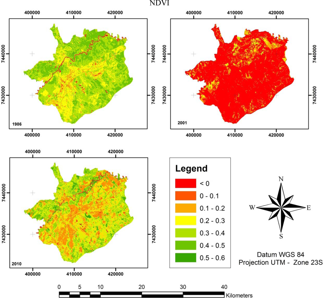
Figure 7.
Probability density function calculated from the Monte Carlo Method (MCM) of the Normalized Difference Vegetation Index (NDVI).
Figure 7.
Probability density function calculated from the Monte Carlo Method (MCM) of the Normalized Difference Vegetation Index (NDVI).
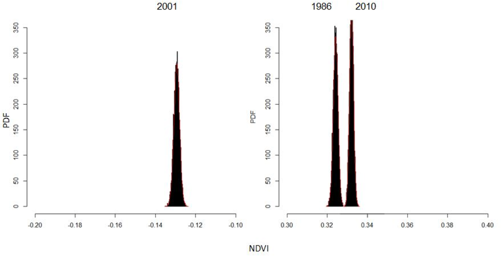
Figure 8.
NDWI calculated from the image of TM/Landsat 5 for 1986, 2001, and 2010.
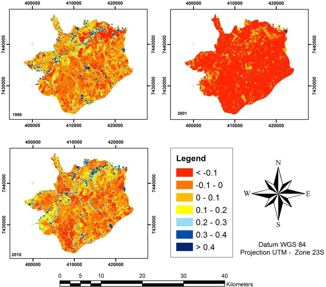
Figure 9.
Probability density function calculated from the MCM of the NDWI.

Figure 10.
NDBI calculated from the image of TM/Landsat 5 for 1986, 2001, and 2010.
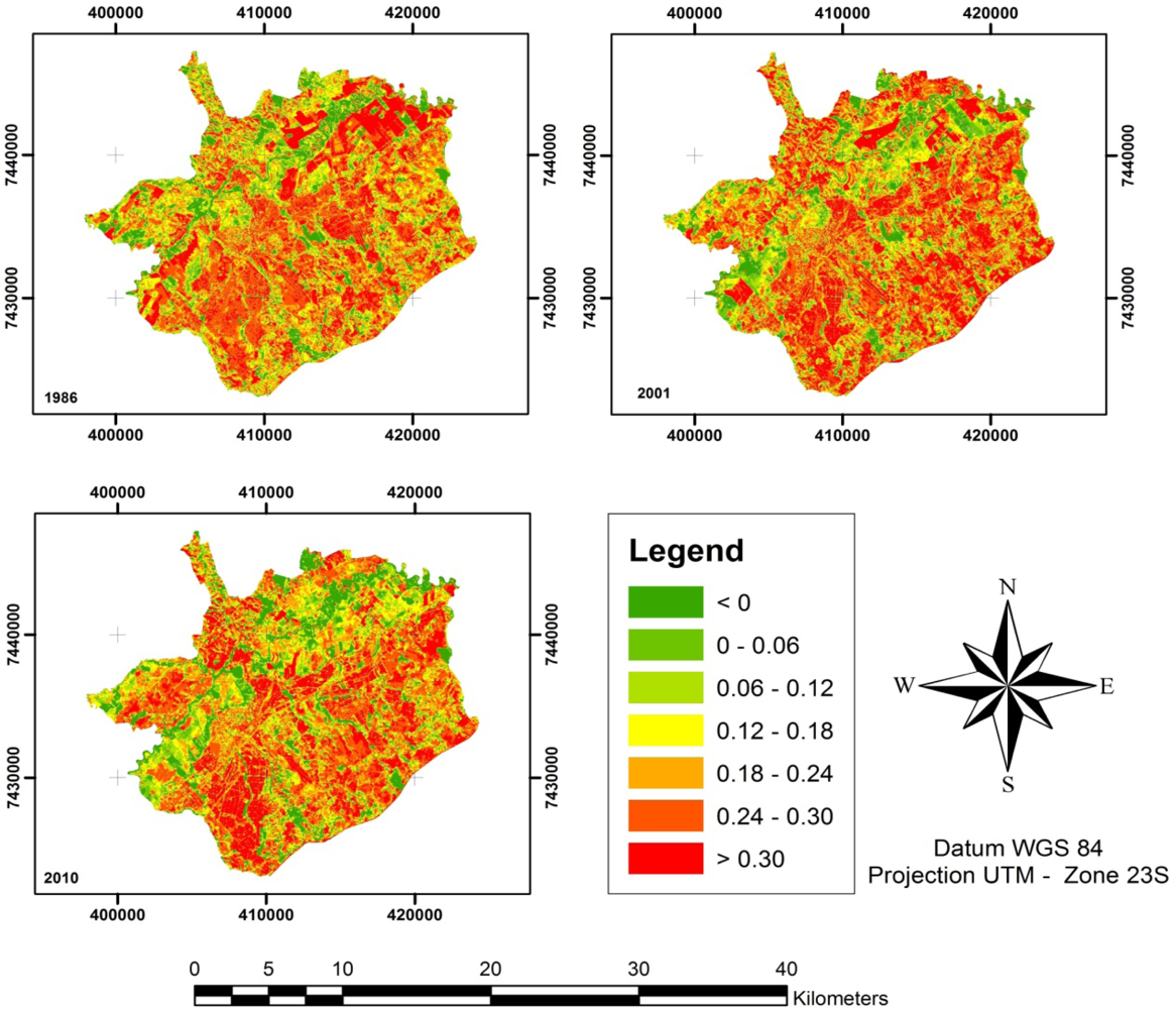
Figure 11.
Probability Density Function calculated from the MCM of NDBI.

Figure 12.
Probability density function calculated from the MCM of land surface temperature.


Table 1.
Correlation matrix of changes in temperature and land cover classes during the analyzed time period.
| <17°C | 17–19°C | 19–21°C | 21–23°C | 23–25°C | 25–27°C | 27–29°C | 29–31°C | 31–33°C | >33°C | urb. | veg. | bar. | wat. | |
|---|---|---|---|---|---|---|---|---|---|---|---|---|---|---|
| <17°C | 1.00 | 0.68 | 0.88 | 1.00 | −0.88 | −0.91 | −0.91 | −0.91 | −0.90 | 0.22 | −0.44 | 0.58 | −0.90 | 0.82 |
| 17–19°C | 1.00 | 0.95 | 0.61 | −0.94 | −0.92 | −0.92 | −0.92 | −0.93 | −0.57 | −0.96 | 0.99 | −0.93 | 0.98 | |
| 19–21°C | 1.00 | 0.83 | −1.00 | −1.00 | −1.00 | −1.00 | −1.00 | −0.28 | −0.81 | 0.90 | −1.00 | 0.99 | ||
| 21–23°C | 1.00 | −0.83 | −0.87 | −0.87 | −0.87 | −0.86 | 0.31 | −0.35 | 0.51 | −0.85 | 0.76 | |||
| 23–25°C | 1.00 | 1.00 | 1.00 | 1.00 | 1.00 | 0.27 | 0.81 | −0.90 | 1.00 | −0.99 | ||||
| 25–27°C | 1.00 | 1.00 | 1.00 | 1.00 | 0.20 | 0.77 | −0.87 | 1.00 | −0.98 | |||||
| 27–29°C | 1.00 | 1.00 | 1.00 | 0.19 | 0.76 | −0.86 | 1.00 | −0.98 | ||||||
| 29–31°C | 1.00 | 1.00 | 0.20 | 0.76 | −0.86 | 1.00 | −0.98 | |||||||
| 31–33°C | 1.00 | 0.23 | 0.78 | −0.88 | 1.00 | −0.99 | ||||||||
| >33°C | 1.00 | 0.78 | −0.66 | 0.24 | −0.38 | |||||||||
| urb. | 1.00 | −0.99 | 0.79 | −0.87 | ||||||||||
| veg. | 1.00 | −0.88 | 0.94 | |||||||||||
| bar. | 1.00 | −0.99 | ||||||||||||
| wat. | 1.00 |
| Temp. | NDWI | NDVI | NDBI | |
|---|---|---|---|---|
| Temp. | 1.00 | 0.50 | 0.96 | −0.20 |
| NDWI | 0.50 | 1.00 | 0.74 | −0.95 |
| NDVI | 0.96 | 0.74 | 1.00 | −0.48 |
| NDBI | −0.20 | −0.95 | −0.48 | 1.00 |
| Temp. | NDWI | NDVI | NDBI | |
|---|---|---|---|---|
| Temp. | 1.00 | 0.87 | 0.52 | −0.27 |
| NDWI | 0.87 | 1.00 | 0.87 | 0.23 |
| NDVI | 0.52 | 0.87 | 1.00 | 0.68 |
| NDBI | −0.27 | 0.23 | 0.68 | 1.00 |
Table 4.
Correlation matrix of the mean values from the indices and LST in a vegetation cover pattern.
| Temp. | NDWI | NDVI | NDBI | |
|---|---|---|---|---|
| Temp. | 1.00 | 0.86 | 0.80 | −0.49 |
| NDWI | 0.86 | 1.00 | 0.99 | 0.02 |
| NDVI | 0.80 | 0.99 | 1.00 | 0.13 |
| NDBI | −0.49 | 0.02 | 0.13 | 1.00 |
| Temp. | NDWI | NDVI | NDBI | |
|---|---|---|---|---|
| Temp. | 1.00 | 0.46 | 0.52 | 0.81 |
| NDWI | 0.46 | 1.00 | 1.00 | 0.89 |
| NDVI | 0.52 | 1.00 | 1.00 | 0.92 |
| NDBI | 0.81 | 0.89 | 0.92 | 1.00 |
Share and Cite
MDPI and ACS Style
Ogashawara, I.; Bastos, V.D.S.B. A Quantitative Approach for Analyzing the Relationship between Urban Heat Islands and Land Cover. Remote Sens. 2012, 4, 3596-3618. https://doi.org/10.3390/rs4113596
AMA Style
Ogashawara I, Bastos VDSB. A Quantitative Approach for Analyzing the Relationship between Urban Heat Islands and Land Cover. Remote Sensing. 2012; 4(11):3596-3618. https://doi.org/10.3390/rs4113596
Chicago/Turabian StyleOgashawara, Igor, and Vanessa Da Silva Brum Bastos. 2012. "A Quantitative Approach for Analyzing the Relationship between Urban Heat Islands and Land Cover" Remote Sensing 4, no. 11: 3596-3618. https://doi.org/10.3390/rs4113596