Infrared Thermometry to Estimate Crop Water Stress Index and Water Use of Irrigated Maize in Northeastern Colorado

1
Department of Civil and Environmental Engineering, Colorado State University, 1372 Campus Delivery, Fort Collins, CO 80523, USA
2
Department of Soil and Crop Sciences, Colorado State University, Plant Sciences C127, Fort Collins, CO 80523, USA
*
Author to whom correspondence should be addressed.
Remote Sens. 2012, 4(11), 3619-3637; https://doi.org/10.3390/rs4113619
Submission received: 26 September 2012
/
Revised: 14 November 2012
/
Accepted: 15 November 2012
/
Published: 20 November 2012
(This article belongs to the Special Issue Advances in Remote Sensing of Crop Water Use Estimation)
Abstract
:With an increasing demand of fresh water resources in arid/semi-arid parts of the world, researchers and practitioners are relying more than ever on remote sensing techniques for monitoring and evaluating crop water status and for estimating crop water use or crop actual evapotranspiration (ETa). In this present study, infrared thermometry was used in conjunction with a few weather parameters to develop non-water-stressed and non-transpiring baselines for irrigated maize in a semi-arid region of Colorado in the western USA. A remote sensing-based Crop Water Stress Index (CWSI) was then estimated for four hourly periods each day during 5 August to 2 September 2011 (29 days). The estimated CWSI was smallest during the 10:00–11:00 a.m. and largest during the 12:00–13:00 p.m. hours. Plotting volumetric water content of the topsoil vs. CWSI revealed that there is a high correlation between the two parameters during the analyzed period. CWSI values were also used to estimate maize actual transpiration (Ta). Ta estimates were more influenced by crop biomass rather than irrigation depths alone, mainly due to the fact that the effects of deficit irrigation were largely masked by the significant precipitation during the growing season. During the study period, applying an independent remotely sensed energy balance model showed that maize ETa was 159 mm, 30% larger than CWSI-Ta (122 mm) and 9% smaller than standard-condition maize ET (174 mm).
1. Introduction
Worldwide, irrigated agriculture is a major contributor to food production. In the USA, for example, only 7.5% of all land under cultivation was irrigated in 2007. But this rather small portion generated $78.3 billion of revenue, which accounted for 55% of the total amount of agricultural crop sale in the same year [1]. The majority (about 75%) of US irrigated land is located in the seventeen Western States, where recent population growth and scarcity of fresh water resources have been exacerbating the challenge of supplying irrigation water demands as well as water for the increasing demands from municipalities and the industrial sector in this arid/semi-arid region. In addition, some of the predicted consequences of climate change for the Western US, such as the change in precipitation pattern, higher temperatures, and prolonged droughts, suggest that decision makers will be faced with even more challenging, and perhaps less studied, issues in the near future. In such an environment, the most promising approach toward a sustainable and cooperative management of agricultural water resources seems to be through improving agricultural water productivity. Producing “more crop per drop”, however, cannot be achieved without having a comprehensive knowledge of crop water status to determine appropriate irrigation rates and timing.
Crop Water Stress Index (CWSI) is a widely used indicator that provides an estimate of crop water status with respect to minimum and maximum levels of stress that can occur due to availability or unavailability of water. CWSI can be estimated using the following equation [2,3]:
where dT is the temperature difference between canopy and air (Tcanopy − Tair) and the subscripts m, LL, and UL represent measured, lower limit (non-water-stressed), and upper limit (severely-stressed) of dT, respectively. Upper and lower limits of dT can be estimated through either the empirical [2] or the theoretical approach [3]. The empirical approach is based on the fundamental assumption that there is a linear relationship between dTLL and vapor pressure deficit (VPD) for a given non-water-stressed crop under a specific climatic condition. Likewise, there is a linear relationship between dTUL and the vapor pressure gradient (VPG) for the same crop when its transpiration is halted due to severe water stress:
where “m” and “b” are slope and intercept of the linear relationship, respectively. VPG is estimated as the difference between saturated vapor pressure at air temperature and at a higher temperature equal to air temperature plus the coefficient “b”.
Equations (2) and (3), also known as non-water-stressed and non-transpiring baselines, respectively, have been previously developed for maize (Zea mays L.) under a wide range of climatic conditions, from semi-arid [4] to sub-humid/sub-tropical [5]. Taghvaeian et al.[6] applied seven of these previously developed baselines to a subset of data from this research experiment. Estimated CWSI for a single one-hour period (12:00–13:00 p.m. MST) was highly variable among implemented methods. Baselines developed under climatic conditions similar to that of the study area in Northeastern Colorado were more successful in appropriately bounding upper and lower limits of dTm, while baselines developed under different climatic conditions had different “m” and “b” coefficients for Equations (2) and (3). In the present study, non-water-stressed and non-transpiring baselines were developed for maize planted under a limited irrigation regime in a semi-arid area of Northeastern Colorado. The results were used along with estimates of several weather parameters and remote sensing-based dTm to estimate CWSI during four different hourly periods in a given day.
Increasing agricultural water productivity is strongly dependent on the ability to accurately estimate the appropriate amount and timing of water application, which is also known as the practice of irrigation scheduling. Although CWSI-based criteria have been extensively used for irrigation scheduling [5–9], they can only provide an answer to the question of “when to apply water.” In other words, while irrigation timing can be identified through setting specific CWSI thresholds, the irrigation amount needs to be estimated based on other methods such as soil water balance [8]. However, if a unique relationship could be established between remote sensing-based CWSI and soil water content, this easy-to-apply method could also be used to answer the question of “how much water to apply” in a spatial fashion to cover large agricultural areas providing insight into the within field and among fields spatial variability of crop water status and use. When Jackson et al.[3] presented the theoretical CWSI approach, they also stated that the consumed fraction of soil extractable water and CWSI had similar trends. But plotting these two variables against each other did not yield a unique relationship. This was mainly due to the fact that extractable water was estimated for the constant upper 1.1 m of soil, while root depth was not constant during the growing season. Nielsen and Anderson [10] used a neutron probe to measure soil water content for the top 30 cm layer of a silt loam soil planted to sunflower and then divided the results by volumetric water content at field capacity, of the same layer, to calculate relative available water (RAW). The correlation between resulted RAW and CWSI values was statistically significant, with a quadratic regression curve that had a high coefficient of determination (0.89). Based on the developed curve, CWSI increased from zero to unity as RAW decreased from about 0.70 to 0.45, respectively [10]. As an attempt to evaluate the possibility of predicting soil water availability using infrared thermometry of crop canopy, the relationship between maize remotely sensed CWSI and soil volumetric water content (VWC) was also investigated in this study.
Another approach to approximate irrigation requirement using CWSI is to estimate crop water consumption based on this indicator. If the amount of water that has been used by the studied crop since the last irrigation/precipitation event is known (monitored using the remote sensing-based CWSI), the amount of water that needs to be applied to fully and/or partially replenish this used portion can be consequently identified. Jackson et al.[3] showed that CWSI is inversely related to the water use of the crop under consideration (maize in this case) through the following relationship:
where Ta and Tc are crop transpiration rates under actual and standard conditions, respectively. The standard condition is defined as a condition under which the studied crop is disease-free, well-watered, and well-fertilized [11]. Tc can be obtained for each crop by multiplying its basal crop coefficients (Kcb) by the reference (grass- or alfalfa-based) ET values. Since CWSI is a dimensionless parameter, Ta has the same units as Tc (e.g., mm·d−1).
The reason that the above equation predicts actual transpiration and not actual evapotranspiration (ETa) is that CWSI estimates are based on canopy thermometry and characteristics of underlying soil are not included. In addition, Equation (4) was derived from an energy balance equation that was defined at crop canopy level and thus does not incorporate any evaporation from the soil background. Evaporation from the soil surface occurs after a wetting event and its duration is limited to one to three days depending on soil type and environmental conditions. Therefore, Ta approaches the definition of ETa between irrigation events. The last objective of the present experiment involved the estimation of maize transpiration by applying Equation (4). To validate CWSI-Ta results, they were compared with ETa estimates from a remotely sensed surface energy balance model. These objectives complement the initial goals of this study that were mentioned earlier in this section: (a) developing non-water stressed and non-transpiring baselines for irrigated maize in a semi-arid climate (Northeastern Colorado); (b) calculating CWSI during the study period based on infrared thermometry data that were collected at different times of the day; and, (c) investigating the relationship between CWSI and VWC of a top layer of the soil.
2. Methods and Materials
2.1. Experimental Layout
The study area was the Lower South Platte Project Research Farm (Latitude: 40.767°, Longitude: −103.044°, Elevation: 1,166 m), located on the flood plains of the nearby South Platte River and close to the city of Iliff in Northeastern Colorado (Figure 1).
The typical soil profile consisted of a Clay-Loam-textured topsoil that was highly variable in depth (0.6–1.3 m), laid over mottled sand and gravel layers. Maize seeds (DKC52-59 Brand, DEKALB ®) were planted on 4 May 2011 at an approximate density of 85,500 seed·ha−1, using a four-row planter with row spacing of about 0.8 m. Applications of urea-ammonium nitrate and ammonium polyphosphate fertilizers on the planting date and the day after provided about 160 and 45 kg·ha−1of Nitrogen and Phosphorus, respectively. In addition, 1.61 L·ha−1 of glyphosate herbicide was applied at the same time. After a 163-day long growing season, yield harvest took place on 13 October 2011. Irrigation water was applied using a linear-move sprinkler irrigation system (T-L Irrigation Company, Hastings, NE, USA), while a 3-m deep drainage ditch along the northern edge of the farm removed deep percolated water from the soil. Two limited irrigation treatments were included in this study. The first treatment had two replicates (L-1.1 and L-1.2, hereafter) and received a total amount of 114 mm of water through four irrigation events. The second treatment also had two replicates (L-2.1 and L-2.2, hereafter) but received three irrigations, totaling 89 mm of applied water. The extra irrigation of L-1 treatment occurred in early July, while the other three irrigations occurred at approximately the same time for all treatments in mid-July, late July, and mid-August. This amount of irrigation water was accompanied by a significant amount of precipitation (400 mm) that fell between planting and harvest dates. Table 1 presents the dates and amounts of precipitation and irrigation events. Due to the large number of wetting events, only those that occurred during one week before the beginning and one week after the end of the study period (5 August–2 September 2011) are presented in this table. Maize growth stage changed from R2 (blister) to R6 (physiological maturity) and senescence between the start and end of the study period.
2.2. Instrumentation
The main sensor at each treatment was an IRT (model SI-111, Apogee Instruments, Inc., Logan, UT, USA) with a 44° field of view, an accuracy of 0.2 °C, and a filter that passes radiation only in the thermal part (8–14 μm) of the electromagnetic (EM) spectrum. The IRT was installed on a mast at a 45° angle below horizon (facing south) to avoid viewing any background soil. Installation height was 2.7 m from the ground surface and remained above the canopy at all times, since the maize did not grow taller than 2.0 m. Canopy temperature was scanned with the IRT units every minute and readings were averaged over a 30-min time interval (period). In order to reference the target temperature and to correct readings for any contribution from heat of the sensor itself, the temperature of the IRT body was also measured by a thermistor embedded inside the sensor. Corrected target (i.e., canopy) temperatures were obtained by applying the body temperature correction algorithm provided by the IRT manufacturer (Apogee). Controlling the measurements, measuring and storing the maize canopy temperature, and reporting measured data were all performed using data-loggers (models CR800 and CR1000, Campbell Scientific Inc., Logan, UT, USA).
At treatment L-2.1, the soil water content from the topsoil was also measured using water content reflectometer sensors (model CS616, Campbell Scientific Inc., Logan, UT, USA). This type of sensor measures the travel time of an EM signal that is transmitted along two 300 mm long stainless steel rods. The time it takes the signal to travel the length of the rod and return to the detector (at the sensor head) is then analyzed inside the sensor electronics to estimate the apparent dielectric permittivity of the soil surrounding the rods, which is directly related to the soil volumetric water content (VWC). Two CS616 sensors were inserted into the soil horizontally at an approximate depth of 5.0 cm and about 25.0 cm apart from each other. In order to compute the soil volumetric water content, the travel time measurements of sensors were first corrected for the effect of soil temperature, using the equation provided in the CS616 manual [12]. Soil temperature data were obtained by inserting a soil temperature probe (model TCAV, Campbell Scientific Inc., Logan, UT, USA) close to the CS616 sensors and at the same depth. The TCAV sensor provides soil temperature measurements that are averaged over its four thermocouples. Temperature-corrected travel time data were then converted into soil VWC using the quadratic equation indicated in the CS616 manual [12]. Finally, the estimated VWC was adjusted for the specific soil texture of the study area by applying a calibration equation that was developed for this type of soil under laboratory conditions [13].
2.3. Maize CWSI
The first step in estimating CWSI was to develop the non-water-stressed and non-transpiring baselines for maize under the semi-arid climatic conditions of the study area in Northeastern Colorado. In order to do so, a procedure similar to that implemented in [2] was followed. More specifically, maize-air temperature differential measurements (dTm) that were collected by IRT during one day after two significant precipitations were plotted with their corresponding VPD data. It was assumed that one day after these major wetting events, the soil water deficit was fully replenished and maize had access to sufficient soil water. Thus, non-water-stressed conditions existed and dTm values represented dTLL values. Plotting dTLLvs. VPD for a 24-h period resulted in a curve, which had a linear section during the period of a few hours after sunrise and a few hours before sunset. This linear segment was extracted and used as non-water-stressed baseline. A three-step moving average was run on both dTLL and VPD data prior to plotting them, as per the suggestion in [2]. Required air temperature and humidity data were obtained from an adjacent weather station that was operated and maintained by the “Colorado Agricultural Meteorological Network (CoAgMet)” program at Colorado Climate Center, Colorado State University, Fort Collins, CO, USA. This alfalfa-based weather station was located at the northwest corner of the experimental field. Air temperature and humidity were measured using a Vaisala sensor (model HMP45C, Campbell Scientific Inc., Logan, UT, USA) that was installed at a height of 1.5 m above the ground. Hourly data were downloaded on 16 November 2011, from the CoAgMet website accessible at: http://ccc.atmos.colostate.edu/~coagmet/. Several key weather parameters during the entire growing season (4 May–13 October 2011) and the study period (5 August–2 September 2011) are presented in Table 2.
Estimates of dTUL were obtained using Equation (3) and coefficients that were derived from the linear segment of the dTLL-VPD curve. Finally, upper and lower limits of dT were entered into Equation (1) along with corresponding dTm measurements during four one-hour periods each day to estimate maize hourly CWSI. However, the empirical approach of the CWSI method is only valid under clear-sky conditions, since cloud cover could have a significant effect on crop temperature. In this study, Relative Shortwave Radiation (RSR) was used to verify the presence of such a condition during the study period. RSR is the ratio of measured shortwave solar radiation (Rs) to calculated clear-sky radiation (Rso). Rs was obtained from the measurements of a pyranometer (model LI-200X, LI-COR Biosciences, Lincoln, NE, USA) installed at the CoAgMet weather station at 2 m height. Rso was estimated based on a procedure and equations explained in [14]. It was assumed that cloud-free conditions existed only when RSR was larger than 0.70. The 30% difference between Rs and Rso was allowed to account for Rs underestimation errors caused by the presence of dirt on the pyranometer’s dome and to account for some haze presence in the atmosphere. Underestimating the effect of atmospheric optical thickness on attenuating solar radiation can also have a similar effect by yielding larger Rso and consequently smaller RSR estimates. For each one-hour time frame during which RSR was less than the identified threshold, the CWSI values from previous and next days (at the same hour) were averaged and used. Out of 29 days of study, only four days had RSR values less than 0.7.
2.4. Maize Water Use
Maize hourly Tc was obtained by multiplying maize Kcb by the hourly alfalfa-based reference ET (ETr) values. Hourly ETr was calculated using weather data collected at the adjacent CoAgMet station and through the ASCE standardized alfalfa reference ET Penman-Monteith equation [14]. Estimates of Kcb were obtained from values presented in [15]. These Kcb values were originally developed at Kimberly, Idaho to be used with 1982 Kimberly-Penman ETr. However, values presented in [15] have been modified to be used with ASCE standardized Penman-Monteith ETr. Twenty-one Kcb values are reported for the beginning and end of 20 intervals, with half of them occurring before and the other half occurring after reaching the effective full cover. Tc values resulted from multiplying Kcb and ETr were entered into Equation (4) along with CWSI estimates in order to calculate hourly maize Ta. However, CWSI should only vary between two theoretical limits of zero and unity in order to obtain reasonable results from this equation. CWSI values greater than one translate into negative water use estimates, while values less than zero convert into Ta rates higher than the Tc rate. Meeting this zero-to-unity range criterion depends on how accurate the baselines are defined. However, these thresholds were applied to estimated CWSI in order to ensure that input values did not violate the range criterion.
Hourly CWSI-Ta values were compared with hourly ETa estimates of a Remotely-sensed Surface Energy Balance (RSEB) model on four dates during the study period. The implemented RSEB model was specifically developed for maize planted in central Iowa, USA [16]. Remotely sensed input data into this model was comprised of surface reflectance and radiometric temperature data that were collected using a hand-held multispectral radiometer equipped with a separate IRT. More details on collecting radiometer/IRT data and running the model are explained in [17]. There are several major differences between the CWSI and the RSEB approaches. The first difference lies in the fact that the CWSI was based on canopy temperature, while the implemented RSEB model also incorporated surface reflectance in the visible and near infrared portions of the EM spectrum. In addition, radiometric surface temperatures used in CWSI were detected by IRT’s that had a 45° viewing angle in order to view only maize canopy; measuring canopy temperatures. In contrast, input data into the RSEB model were collected by a radiometer/IRT that had a nadir-viewing angle, resulting in the presence of both maize canopy and some underlying soil in the sensor field of view. These differences explain why the remote sensing-based CWSI model provided an estimate of crop transpiration, while RSEB results also included evaporation from soil surfaces (if any after a wetting event). Another difference that may play a role was that stationary CWSI-IRTs were directed to the south; viewing mostly shaded leaves (sunlit leaves were facing away from the IRT). The nadir looking handheld radiometer/IRT, on the other hand, viewed both sunlit and shaded leaves.
Although hourly estimates of maize Ta are useful in determining crop water requirement, irrigation managers are usually more interested in estimates that represent periods longer than hourly. As a result, several methods have been developed to extrapolate hourly water consumption rates to daily and seasonal estimates. One method that has been mainly utilized by recent RSEB models is known as “the alfalfa reference ET fraction” or ETrF, which is based on the assumption that the ratio of ETa to ETr at the time of data collection remains constant during the day [18]. Once this ratio is calculated based on hourly data, it can be multiplied by daily estimates of ETr to provide an approximation of ETa on daily basis. A similar approach, which we called “standard-condition crop ET fraction” or ETcF (Ta/Tc), was employed in this study to extrapolate CWSI-based estimates. It was assumed that the ratio of hourly CWSI-Ta to hourly Tc was equal to the ratio of daily Ta and Tc. Rearranging Equation (4) shows that for this assumption to be valid, CWSI value estimated for the hour of data collection should be equal to average CWSI during the day. However, previous experiments do not suggest any specific time frame that would meet this requirement. They show, however, that CWSI ranges from a minimum value during early morning hours to a peak that usually occurs after solar noon. Thus, the ETcF method will overestimate and/or underestimate daily Ta if canopy temperature data are collected during early morning or afternoon hours, respectively. It is very likely that CWSI during one of the hourly periods between these two extremes is close to daily average CWSI. The authors acknowledge that not knowing the average daily CWSI introduces some error that needs to be considered when interpreting computed water use estimates. However, ETcF is the only approach available for extrapolating hourly CWSI-Ta estimates. Further research should be conducted in order to establish modifications to this method or to recommend a specific time frame for data collection over which hourly CWSI would represent the average daily value of this parameter.
Daily RSEB-ETa values were also estimated from extrapolating hourly values using the ETrF method. Finally, cumulative maize water use was estimated for the entire study period based on both the CWSI and the RSEB method. For the CWSI, daily Ta values that were extrapolated from each of the one-hour periods were summed over the entire study period. As a result, a different estimate of cumulative maize water use was obtained for each hourly period considered. Since radiometer data were collected only on four dates during the study period, RSEB-ETa values were interpolated for the days in between data collection dates by assuming that ETrF had a linear variation between the two consecutive measurement dates [18].
3. Results and Discussion
3.1. Maize CWSI
Maize dTLL, for the semi-arid climate of the study area in Northeastern Colorado, was plotted with VPD for all four experimental plots using data from two dates that each occurred after a significant precipitation. As an example, Figure 2 shows the resulting graph for plots L-1.1 and L-1.2, using the data collected on 15 August 2011 (R3/R4 stages).
The pattern observed in Figure 2 is very similar to graphs presented in [2], where dTLL increases with increasing VPD for two to three hours after sunrise. At this point in time, incoming shortwave solar irradiance is large enough for stomata to fully open and allow for a transpiration rate equal to the Tc rate (provided sufficient water content is present in the soil root zone). Consequently, dTLL decreases linearly with increasing VPD until a few hours before sunset, when dTLL starts behaving differently (Figure 2). The dotted black line in Figure 2 presents the non-water-stressed baseline that was developed by Idso [19] for maize grown in a semi-arid area of Arizona, USA. As it can be seen, the linear section of the dTLL-vs.-VPD plot in this study matches closely with this previously developed baseline. This linear section spans over a five-hour period between 10:00 and 15:00 (MST: Mountain Standard Time). However, only the data from two hours before and two hours after solar noon were considered for developing the non-water-stressed baseline and for conducting further analyses. Since solar noon was within a few minutes from 12:00 p.m. during the study, the selected four-hour period was from 10:00 to 14:00 (MST).
Fitting a linear line to the dTLL-vs.-VPD data obtained during this four-hour period on the mentioned two dates and over all treatments resulted in the following relationship:
Coefficients of Equation (5) are close to those developed for maize and presented in [19] (m = −1.97, b = 3.11) and [20] (m = −1.97, b = 2.14). This similarity explains the observation of Taghvaeian et al.[6] that in comparison with five other previously developed baselines, these two sets of coefficients (from [19,20]) had the best performance in accurately defining upper and lower limits of dTm values measured in this study. During the study period (5 August to 2 September), average dTLL estimated from Equation (5) was −1.5, −2.4, −3.1, and −3.8 °C during the 10–11, 11–12, 12–13, and 13–14 h, respectively. The increase in absolute value of dTLL is due to the increase in VPD from a.m. to p.m. hours. The non-transpiring baseline was also defined using coefficients similar to those of Equation (5). Average dTUL over the same period increased from 4.0 °C at 10–11 h to 4.3 °C at 13–14 h, at a constant rate of 0.1 °C·h−1. These values are similar to the average dTUL of 4.6 °C, measured from 3 August to 12 September 1995 over a severely stressed maize plot under a Mediterranean semi-arid climate [7].
Finally, the remote sensing-based CWSI was calculated for each of the one-hour periods between 10:00 and 14:00 (MST). As expected, each time frame resulted in a slightly different CWSI value estimate. Figure 3 depicts the variation in hourly CWSIs for two plots, L-1.2 and L-2.2, during the four weeks of study. The depth of applied water through either irrigation or precipitation is also showed as vertical bars on a separate ordinate. According to Figure 3, maize experienced almost no stress during the first week of the study (R2/R3 stages). This is mainly due to the fact that 30.5 mm of rain fell on the field on 4 August 2011. This precipitation event was followed by two more rainfalls during the first week that were not significant in amount, but probably enough to compensate for part of the 4 August rainfall that was evaporated from the soil surface or transpired by maize. CWSI then increased to less than 0.2 before the next precipitation event happened on 14 August 2011. The effect of this precipitation on lowering stress levels is obvious in Figure 3. After this event, however, CWSI increased steadily until 25 August, which is when the average daily air temperature reached its maximum value of 27.9 °C during the study period. Decreased air temperatures and 21 mm of rainfall on 29 August caused CWSI to remain constant or decrease over the last week of the study (R6 stage). Based on the results, the irrigation that occurred on 21 August for these plots was not able to reverse the trend in CWSI variation, even though it provided 25 mm of water. Table 3 presents the mean and median hourly CWSI values for all experimental plots during study period.
For each plot, the average CWSI increased from a lower value during the 10–11 h to a maximum value during the 12–13 h and then it decreased slightly during the last hour (13–14). Irmak et al.[7] also stated that the period between 12:00 and 13:00 was when CWSI was largest and thus, CWSI-based irrigation scheduling should use the data collected during this period of the day. They also found out that seasonal average of CWSI for maize planted under Mediterranean semiarid climate should stay below 0.22 in order to avoid any yield loss [7]. This is similar to another previous finding that no significant yield loss occurred under an irrigation scheduling based on CWSI threshold of 0.20 [20]. Based on the results, irrigation treatments did not have a significant effect on water stress experienced by maize. Average CWSI over all hourly periods was 0.27 and 0.29 for treatments L-1 and L-2, respectively.
3.2. CWSI and Soil Water Content
Soil VWC was plotted with CWSI values for each of the four hourly periods. As explained before, VWC data were collected only at plot L-2.1 at a depth of 5.0 cm from the soil surface. Recorded values were then corrected for the effect of soil temperature and were calibrated for the soil texture type using relationships developed in laboratory for the same type of soil [13]. Plotted data were limited to a 13-day period that occurred during the last two weeks of August (R5/R6 stages) and in between two significant precipitation events (Figure 4). The topsoil VWC was highly correlated to maize CWSI for all studied hourly periods. When the data from all periods were combined, the relationship between VWC and CWSI was best described by the following second order polynomial:
Based on Equation (6), VWC would be equal to or greater than 28.31% at no stress and equal to or less than 22.18% at fully stressed conditions. This observation reveals that it only takes about 6% variation in total topsoil VWC to go from maize non-water-stressed to non-transpiring limits for the clay loam soil in Northeastern Colorado.
Several important points should be considered in interpreting and utilizing the CWSI-vs.-VWC relationship presented in this study. First of all, VWC data that were used in developing Equation (6) represent soil water content condition in only a thin top layer of the soil, which has larger diurnal temperature variations and it is also more subject to evaporation from the soil surface. As a result, the relationship would be different if the soil water content profile over the entire root zone (e.g., one meter) was included in the analysis. Such a relationship would be truly capable of approximating the amount of irrigation water that needs to be applied at a specific CWSI value and a specific soil type. This approach, however, has faced challenges in the past, as the effective root depth of crop changes during the season [3]. The authors believe that a feasible solution to this issue is to divide the growing season into shorter growth stages. The CWSI-vs.-VWC relationships developed over these shorter periods will have higher statistical confidence not only due to the fact that estimates of VWC over the root zone will be improved, but also because crops have different sensitivities to water stress at different growth stages.
Another modification that will considerably increase the utility of CWSI in predicting irrigation requirement is to replace soil VWC with soil matric potential, which would yield a relationship that is universal to all soil types. Then, for a specific soil type, the relationship between soil matric potential and soil water content would be needed, i.e., the soil water characteristic curve. The second point that should be noted in interpreting Equation (6) is that the data shown in Figure 4 were collected during a 13-day period when maize was at R5/R6 (dent and physiological maturity) stage of growth. Since this crop (similar to other crops) has a variable sensitivity to water stress during different growth stages, developed relationships cannot be used to estimate VWC at other growth stages. For example, maize is believed to be more sensitive to water availability during VT (tasseling) and R1 (silking) stages. Thus, a smaller range of VWC values may have been observed if the data in this study were collected during these two stages. Similarly, it is expected that the CWSI-VWC curve would shift toward larger CWSI values after the R6 stage, since transpiration (the main process responsible for cooling the canopy) drops down due to crop senescence.
3.3. Maize Water Use
As the first step toward evaluating the performance of the CWSI method in estimating maize water use, hourly CWSI-Ta and RSEB-ETa were compared on four dates when multispectral radiometer data were collected (Figure 5). Hourly data were used for comparison in order to exclude any effect that extrapolating from hourly to daily values may have had on water use estimates.
The results showed that the difference between the two estimates increased over time as the crop transitioned from R2 into R6 phases. For the first date (5 August, R2 stage), RSEB-ETa was 1% smaller than CWSI-Ta for plot L-2.2 and about 6% larger for the other plots. A high Soil Adjusted Vegetation Index (SAVI) of 0.68 indicates that the canopy was at full cover on this date. Thus, it is not surprising that Ta and ETa estimates are very close to each other, since both nadir-looking radiometer and oblique IRT were viewing only plant leaves. On the second date (15 August, R3/R4 stages) ETa was from 1% to 7% larger than Ta for all plots. Average SAVI was still rather high (0.63) on this date, meaning that the canopy remained close to full cover, as previous studies show that maize reaches full cover at a SAVI value of 0.64 [21], which would correspond to a value of leaf area index (LAI) of 3.0 m2·m−2 or larger. On the third comparison date (31 August, R5/R6 stages), maize had entered into the maturity/senescence phase, and the growth stage was also more variable among treatments. While Plots L-1.1 and L-2.2 had an average SAVI value of 0.55, Plots L-1.2 and L-2.1 showed more signs of senescence and had an average SAVI of 0.43. So the hand-held multispectral radiometer was viewing both canopy and soil surface. On this date, ETa estimates were 13% larger than Ta for the former two plots, but they were 63% larger for the latter two plots. It is worth mentioning that this date was preceded by a significant precipitation event (21.1 mm) that occurred two days earlier. The soil surface was still saturated when the field was visited for data collection and thus evaporation from the soil surface was taking place at a relatively high rate. On the last date (5 September R6 stage), all treatments were partially senesced and the average SAVI dropped to 0.37, resulting in ETa estimates that were from 2.6 to 3.8 times larger than the Ta estimates.
Chávez et al.[16] showed that RSEB-ETa results were in good agreement with estimates of maize ET from eddy-covariance latent heat flux towers, having a small error (mean ± std dev) of −9.2 ± 39.4 W·m−2. A unit conversion using the average latent heat of vaporization that was estimated during data collection periods showed that this error is equivalent to −0.01 ± 0.06 mm·h−1. Taking RSEB-ETa results as a reference, the Mean Absolute Error (MAE) of CWSI-Ta was calculated as 0.03, 0.03, and 0.10 mm·h−1 on the first three comparison dates, respectively. Limiting the analyses to plots that had larger biomass and therefore less exposed soil (L-1.1 and L-2.2) decreased MAE to 0.02, 0.02, and 0.05 mm·h−1, respectively. Since these MAE estimates are obtained by comparing CWSI-Ta values to modeled (and not measured) values, they may not be regarded as actual errors of CWSI results. However, it is perhaps safe to conclude that the remote sensing-based CWSI method can yield water use estimates that are as accurate as the RSEB results, since MAE values are all within the accuracy range of the RSEB algorithm. This is a promising finding, as running RSEB models is by far more complicated and time-consuming than the CWSI approach.
Daily maize Ta estimates during the study period showed a pattern similar to what was observed in comparing hourly Ta and ETa estimates. Plots L-1.1 and L-2.2 that had more biomass and later senescence transpired more water than Plots L-1.2 and L-2.1. Ta rates estimated for the former two plots were also closer to their corresponding ETa rates compared to the latter two plots. Figure 6 presents time series of maize water use for all of the studied plots. This figure is succeeded by Table 4, which summarizes average and cumulative water use estimates for all treatments/plots and based on all implemented methods. Cumulative maize transpiration, averaged over all one-hour periods and the two plots with denser maize canopies (L-1.1 and L-2.2), was 130.9 ± 5.3 mm during the study period. Cumulative maize transpiration for the two plots with sparser maize canopies was 113.6 ± 3.0 mm for the same period. Estimated standard-condition crop transpiration (Tc) was 169.0 mm during the same period, suggesting that maize did experience some water stress, but it was not close to the level that was targeted by applying equal to or less than 114 mm of irrigation water during the growing season. This was due to the fact that limited amounts of irrigation application were accompanied by a higher-than-normal precipitation of 400 mm during the growing season. Such a significant amount of precipitation also masked the effects of different irrigation treatments. As expected, CWSI-Ta estimates were largest and smallest when calculated based on data collected during 10–11 and 12–13 time frames, respectively. Although the magnitude of the difference was not significant (total Ta for 12–13 was from 5% to 10% smaller than 10–11 results among studied plots), these variations should still be considered when selecting a time frame for remote sensing data collection (i.e., IRT data).
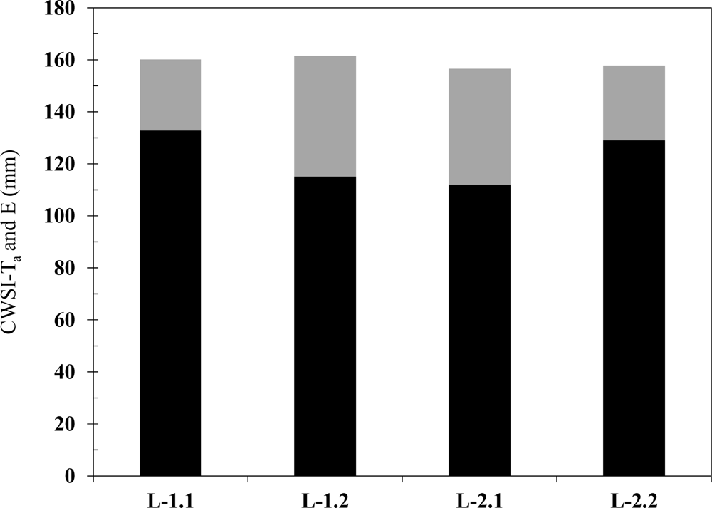
Maize ETa based on the implemented RSEB model did not have a similar behavior to Ta approximations of the CWSI method. ETa estimates were much closer among plots, with Plots L-2.1 and L-1.2 having the smallest (156.6 mm) and the largest (161.5 mm) evapotranspiration, respectively. Since comparing hourly CWSI-Ta and RSEB-ETa showed that both methods generated similar results when only maize leaves were viewed, the different behavior and larger magnitude of total ETa compared to Ta was most probably due to the effect of water evaporation from the soil surface. As all plots received rather frequent water applications (irrigation or precipitation), lower transpiration at sparser locations was compensated by higher evaporation, resulting in comparable ETa estimates. During the 29 days of study, maize total transpiration (averaged over all hourly periods) was 132.8, 115.1, 112.0, and 129.1 mm for L-1.1, L-1.2, L-2.1, and L-2.2 plots, respectively (Figure 7). Maize average RSEB-ETa for all plots was 159.0 mm, 9% smaller than the standard-condition maize ETc (173.9 mm) during the same period. Ignoring the inherent error in the results of each method, average water evaporation from the soil surface (E) can be estimated by subtracting CWSI-Ta from RSEB-ETa. Estimated E was 36.8 mm on average, which accounts for 23% of the total ETa during the study period.
The ratio of maize ETc to ETa was 1.09, significantly smaller than the ratio of maize Tc to Ta, which varied from 1.33 to 1.43 among the results of hourly periods. In other words, when compared to their corresponding rates under standard (stress-free) conditions, actual transpiration was more reduced than actual evapotranspiration. This difference may imply that evaluating crop Ta can provide more information on the presence and severity of water stress compared to ETa, which also includes water evaporation from the soil surface. Results found in this study are evidence that remote sensing-based maize water stress can be monitored, using infrared thermometry and weather data, to infer on when to irrigate and how much water to apply.
4. Conclusions
Maize water stress and consumptive use were investigated by conducting a research experiment in Northeastern Colorado, USA, during the summer of 2011. The non-water-stressed baseline developed in this study was similar to those developed by other researchers under similar semi-arid climatic conditions. However, each of the studied hourly periods (10:00–14:00) resulted in a slightly different estimate of remote sensing-based Crop Water Stress Index (CWSI), suggesting that data collection time is a key parameter in utilizing the CWSI approach. A major contribution of this research was in exploring the methods that would enable the use of CWSI not only for identifying irrigation timing, but also for estimating irrigation requirement. The first method was to predict soil water content based on CWSI. When only a thin layer of topsoil was considered, the developed relationship had a high coefficient of determination. However, further research is required to include the entire root zone of the studied crop before such relationships can be used for practical applications.
The second method was to calculate maize actual transpiration (Ta) based on the remote sensing-based CWSI estimates, an analysis that has been rarely performed in previous studies. The hourly CWSI-Ta data were compared with actual evapotranspiration (ETa) values that were obtained by running an independent Remotely-sensed Surface Energy Balance (RSEB) model. The results showed that when input data into the RSEB model were only collected over maize canopy, the difference between the results was well within the accuracy of the RSEB model. Thus, the empirical CWSI approach is as accurate in computing crop water use as the physically based and more computationally intense RSEB model implemented in this study. It should be noted, however, that since the input data into the CWSI method must not be affected by the exposure of underlying soil, this approach in its current form can be applied only to ground-based remotely sensed data (IRT sensor pointing in an oblique angle to capture only canopy temperature), a constraint that limits its application to the farm level. RSEB models, on the other hand, can be applied to air- and space-borne images that cover large agricultural areas with a high variability in crop type, growth stage, and irrigation methods.
In summary, it seems that the remote sensing-based empirical CWSI method is an efficient approach that may be used to perform an accurate irrigation scheduling (timing and amounts). The fact that stress level changes to some extent depending on the time of data collection does not introduce a major challenge for most practical applications. As long as a consistent time frame is used for data collection, CWSI thresholds developed specifically for that time frame could be used for identifying irrigation timing. For example, a more conservative (lower) CWSI threshold can be selected if measurements are taken during earlier hours, while CWSI may be allowed to reach higher levels if data are collected during one hour after solar noon.
Acknowledgments
This research was jointly funded by the Colorado Water Conservation Board, Parker Water and Sanitation District, and the Colorado Corn Growers Association. The authors would like to express their sincere appreciation to Jessica Gerk, David Gleason, Evan Rambikur, and Abhinaya Subedi for their assistance in installing sensors and conducting field work. The authors are also grateful to the anonymous reviewers who contributed to this work by providing constructive comments.
References
- Schaible, G.D.; Aillery, M.P. US Irrigated Agriculture: Water Management and Conservation. In Agricultural Resources and Environmental Indicators, 2012. EIB-98; Osteen, C, Gottlieb, J, Vasavada, U, Eds.; US Department of Agriculture, Economic Research Service: Washington, DC, USA, 2012; pp. 29–32. [Google Scholar]
- Idso, S.B.; Jackson, R.D.; Pinter, P.J., Jr; Reginato, R.J.; Hatfield, J.L. Normalizing the stress-degree-day parameter for environmental variability. Agric. Meteorol 1981, 24, 45–55. [Google Scholar]
- Jackson, R.D.; Idso, S.B.; Reginato, R.J. Canopy temperature as a crop water stress indicator. Water Resour. Res 1981, 17, 1133–1138. [Google Scholar]
- Yazar, A.; Howell, T.A.; Dusek, D.A.; Copeland, K.S. Evaluation of crop water stress index for LEPA irrigated corn. Irrig. Sci 1999, 18, 171–180. [Google Scholar]
- Kar, G.; Kumar, A. Energy balance and crop water stress in winter maize under phenology-based irrigation scheduling. Irrig. Sci 2010, 28, 211–220. [Google Scholar]
- Taghvaeian, S.; Chávez, J.L.; Hansen, N.C. Evaluating Crop Water Stress under Limited Irrigation Practices. Proceedings of the World Environmental and Water Resources Congress 2012: Crossing Boundaries, Albuquerque, NM, USA, 20–24 May 2012; pp. 2149–2159.
- Irmak, S.; Haman, D.Z.; Bastug, R. Corn: Determination of crop water stress index for irrigation timing and yield estimation of corn. Agron. J 2000, 92, 1221–1227. [Google Scholar]
- Nielsen, D.C. Scheduling irrigations for Soybeans with the Crop Water Stress Index (CWSI). Field Crop. Res 1990, 23, 103–116. [Google Scholar]
- Stegman, E.C. Efficient irrigation timing methods for corn production. Trans. ASAE 1986, 29, 203–210. [Google Scholar]
- Nielsen, D.C.; Anderson, R.L. Infrared thermometry to measure single leaf temperatures for quantification of water stress in sunflower. Agron. J 1989, 81, 840–842. [Google Scholar]
- Allen, R.G.; Pereira, L.S.; Raes, D.; Smith, M. FAO Irrigation and Drainage Paper No. 56, Crop Evapotranspiration (Guidelines for Computing Crop Water Requirements); FAO Water Resources, Development and Management Service: Rome, Italy, 2007; p. 300. [Google Scholar]
- Campbell Scientific. Instructional Manual: CS616 and CS625 Water Content Reflectometers (v. 3.12). Available online: http://s.campbellsci.com/documents/us/manuals/cs616.pdf (accessed on 24 May 2012).
- Varble, J.L.; Chávez, J.L. Performance evaluation and calibration of soil water content and potential sensors for agricultural soils in eastern Colorado. Agric. Water Manag 2011, 101, 93–106. [Google Scholar]
- ASCE-EWRI, The ASCE Standardized Reference Evapotranspiration Equation; Task Committee on Standardization of Reference Evapotranspiration, Environment and Water Resources Institute of the ASCE: Reston, VA, USA, 2005; p. 216.
- Allen, R.G.; Wright, J.L.; Pruitt, W.O.; Pereira, L.S.; Jensen, M.E. Water Requirements. In Design and Operation of Farm Irrigation Systems, 2nd ed.; American Society of Agricultural and Biological Engineers: St. Joseph, MI, USA, 2007; p. 850. [Google Scholar]
- Chávez, J.L.; Neale, C.M.U.; Hipps, L.E.; Prueger, J.H.; Kustas, W.P. Comparing aircraft-based remotely sensed energy balance fluxes with eddy covariance tower data using heat flux source area functions. J. Hydrometeorol 2005, 6, 923–940. [Google Scholar]
- Taghvaeian, S.; Chávez, J.L.; Hansen, N.C. Ground-Based Remote Sensing of Corn Evapotranspiration under Limited Irrigation Practices. Proceedings of the 32nd Annual American Geophysical Union Hydrology Days, Fort Collins, CO, USA, 21–23 March 2012; pp. 119–131.
- Allen, R.G.; Tasumi, M.; Trezza, R. Satellite-based energy balance for mapping evapotranspiration with internalized calibration (METRIC)-model. J. Irrig. Drain. Eng 2007, 133, 380–394. [Google Scholar]
- Idso, S.B. Non-water-stressed baselines: A key to measuring and interpreting plant water stress. Agric. Meteorol 1982, 27, 59–70. [Google Scholar]
- Steele, D.D.; Stegman, E.C.; Gregor, B.L. Field comparison of irrigation scheduling methods for corn. Trans. ASAE 1994, 37, 1197–1203. [Google Scholar]
- Bausch, W.C. Soil background effects on reflectance-based crop coefficients for corn. Remote Sens. Environ 1993, 46, 213–222. [Google Scholar]
Figure 1.
Location of the study area and instrumentation sites.
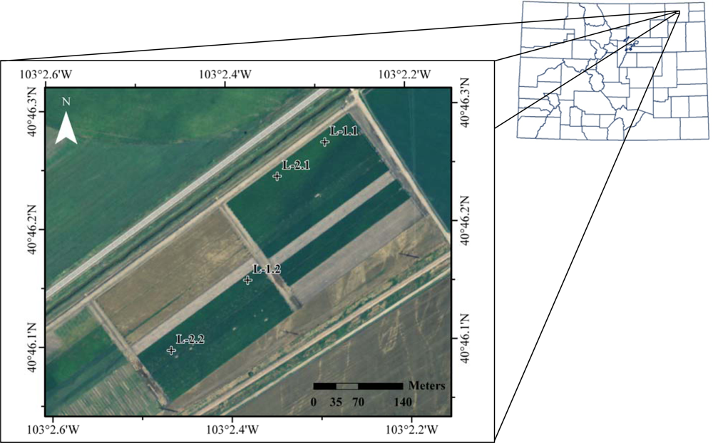
Figure 2.
Graphs of hourly dTLL-vs.-VPD for plots L-1.1 (black arrows) and L-1.2 (gray arrows), overlaid on maize non-water-stressed baseline (dotted black) of Idso [19].
Figure 2.
Graphs of hourly dTLL-vs.-VPD for plots L-1.1 (black arrows) and L-1.2 (gray arrows), overlaid on maize non-water-stressed baseline (dotted black) of Idso [19].
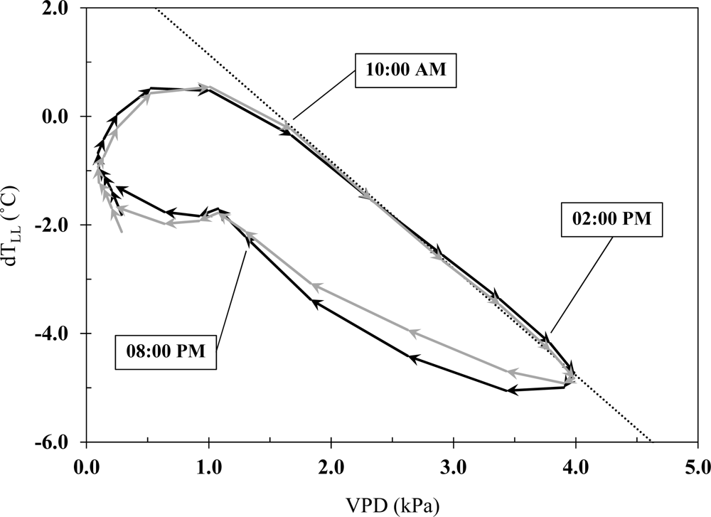
Figure 3.
Hourly graphs of Crop Water Stress Index (CWSI) for plots L-1.2 (left) and L-2.2 (right) during the study period (5 August–2 September 2011).
Figure 3.
Hourly graphs of Crop Water Stress Index (CWSI) for plots L-1.2 (left) and L-2.2 (right) during the study period (5 August–2 September 2011).
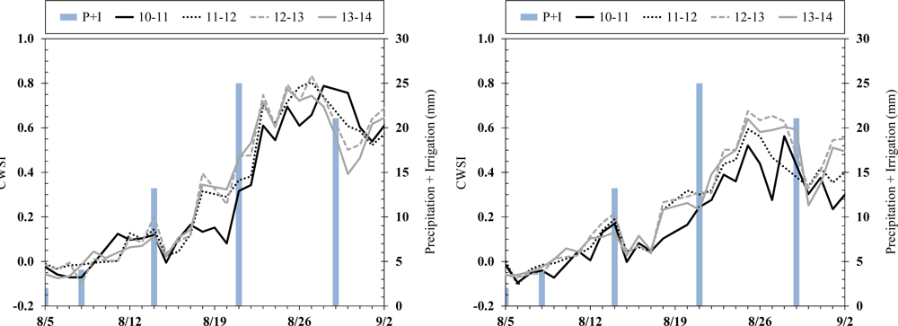
Figure 4.
Scatterplot of CWSI vs. volumetric water content (VWC) for the topsoil at plot L-2.1 during a 13-day period (16 August–28 August 2011).
Figure 4.
Scatterplot of CWSI vs. volumetric water content (VWC) for the topsoil at plot L-2.1 during a 13-day period (16 August–28 August 2011).
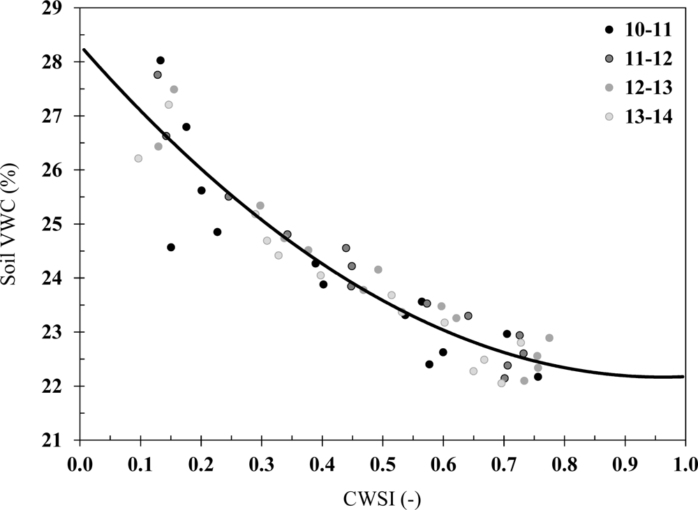
Figure 5.
CWSI-Tavs. remotely-sensed surface energy balance-actual evapotranspiration (RSEB-ETa) estimates for four days in the summer of 2011.
Figure 5.
CWSI-Tavs. remotely-sensed surface energy balance-actual evapotranspiration (RSEB-ETa) estimates for four days in the summer of 2011.
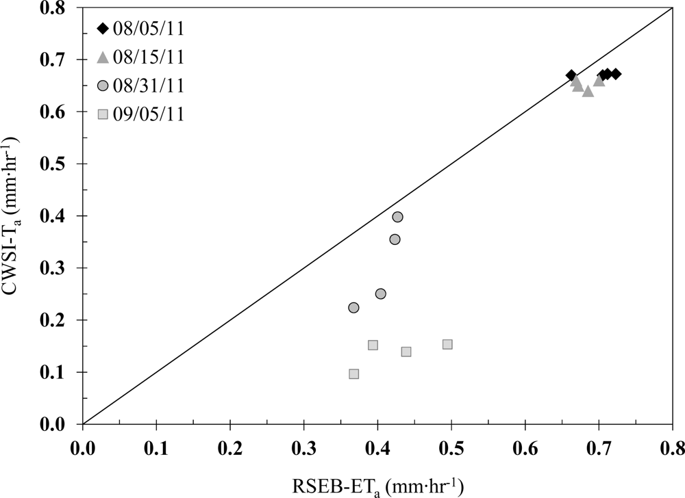
Figure 6.
Daily maize water use for all plots. The green double line is the RSEB-ETa, while black and gray lines represent CWSI-Ta based on each one-hour period.
Figure 6.
Daily maize water use for all plots. The green double line is the RSEB-ETa, while black and gray lines represent CWSI-Ta based on each one-hour period.
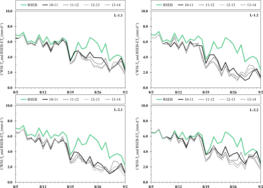
Figure 7.
Total CWSI-Ta (black bars) and average water evaporation from the soil surface (E) (gray bars) during the study period and averaged over all four hours (10–14).
Figure 7.
Total CWSI-Ta (black bars) and average water evaporation from the soil surface (E) (gray bars) during the study period and averaged over all four hours (10–14).

Table 1.
Dates and amounts of precipitation and irrigation events during one week before the beginning and one week after the end of the study period.
| Date | Precipitation (mm) | Irrigation (mm) | |||
|---|---|---|---|---|---|
| L-1.1 | L-1.2 | L-2.1 | L-2.2 | ||
| 07/28/2011 | 38.0 | 38.2 | |||
| 07/29/2011 | 38.0 | 38.0 | |||
| 08/04/2011 | 30.5 | ||||
| 08/05/2011 | 2.0 | ||||
| 08/08/2011 | 4.1 | ||||
| 08/14/2011 | 13.2 | ||||
| 08/20/2011 | 25.0 | 25.0 | |||
| 08/21/2011 | 25.0 | 25.0 | |||
| 08/29/2011 | 21.1 | ||||
| Parameter | Growing Season | Study Period |
|---|---|---|
| Average daily mean Tair | 18.8 (°C) | 23.2 (°C) |
| Average daily max. Tair | 28.7 (°C) | 33.8 (°C) |
| Average daily min. Tair | 9.6 (°C) | 14.1 (°C) |
| Average daily vapor pressure | 1.30 (kPa) | 1.63 (kPa) |
| Average daily min. RH | 28.1 (%) | 23.9 (%) |
| Average daily wind run | 178.2 (km·d−1) | 160.1 (km·d−1) |
| Average daily Solar rad. | 234.3 (W·m−2) | 245.6 (W·m−2) |
| Plot | 10–11 | 11–12 | 12–13 | 13–14 | ||||
|---|---|---|---|---|---|---|---|---|
| Mean | Median | Mean | Median | Mean | Median | Mean | Median | |
| L-1.1 | 0.18 | 0.10 | 0.21 | 0.18 | 0.24 | 0.18 | 0.23 | 0.17 |
| L-1.2 | 0.30 | 0.15 | 0.33 | 0.30 | 0.34 | 0.33 | 0.32 | 0.33 |
| L-2.1 | 0.33 | 0.22 | 0.36 | 0.34 | 0.36 | 0.34 | 0.33 | 0.31 |
| L-2.2 | 0.18 | 0.16 | 0.23 | 0.27 | 0.27 | 0.28 | 0.26 | 0.23 |
| Plot | CWSI-Ta | RSEB-ETa | ETc | |||||||||
|---|---|---|---|---|---|---|---|---|---|---|---|---|
| 10–11 | 11–12 | 12–13 | 13–14 | |||||||||
| Mean | Total | Mean | Total | Mean | Total | Mean | Total | Mean | Total | Mean | Total | |
| L-1.1 | 4.78 | 138.5 | 4.61 | 133.6 | 4.43 | 128.4 | 4.50 | 130.6 | 5.52 | 160.1 | 6.00 | 173.9 |
| L-1.2 | 4.08 | 118.2 | 3.96 | 115.0 | 3.88 | 112.5 | 3.96 | 114.8 | 5.57 | 161.5 | ||
| L-2.1 | 3.95 | 114.7 | 3.80 | 110.1 | 3.75 | 108.7 | 3.95 | 114.6 | 5.40 | 156.6 | ||
| L-2.2 | 4.73 | 137.1 | 4.48 | 130.0 | 4.25 | 123.2 | 4.34 | 126.0 | 5.44 | 157.8 | ||
Share and Cite
MDPI and ACS Style
Taghvaeian, S.; Chávez, J.L.; Hansen, N.C. Infrared Thermometry to Estimate Crop Water Stress Index and Water Use of Irrigated Maize in Northeastern Colorado. Remote Sens. 2012, 4, 3619-3637. https://doi.org/10.3390/rs4113619
AMA Style
Taghvaeian S, Chávez JL, Hansen NC. Infrared Thermometry to Estimate Crop Water Stress Index and Water Use of Irrigated Maize in Northeastern Colorado. Remote Sensing. 2012; 4(11):3619-3637. https://doi.org/10.3390/rs4113619
Chicago/Turabian StyleTaghvaeian, Saleh, José L. Chávez, and Neil C. Hansen. 2012. "Infrared Thermometry to Estimate Crop Water Stress Index and Water Use of Irrigated Maize in Northeastern Colorado" Remote Sensing 4, no. 11: 3619-3637. https://doi.org/10.3390/rs4113619