Arctic Ecological Classifications Derived from Vegetation Community and Satellite Spectral Data

1
Department of Geography, Ryerson University, Toronto, ON M5B 2K3, Canada
2
Department of Geography, Queen's University, Kingston, ON K7L 3N6, Canada
*
Author to whom correspondence should be addressed.
Remote Sens. 2012, 4(12), 3948-3971; https://doi.org/10.3390/rs4123948
Submission received: 4 October 2012
/
Revised: 26 November 2012
/
Accepted: 4 December 2012
/
Published: 10 December 2012
Abstract
:As a result of the warming observed at high latitudes, there is significant potential for the balance of ecosystem processes to change, i.e., the balance between carbon sequestration and respiration may be altered, giving rise to the release of soil carbon through elevated ecosystem respiration. Gross ecosystem productivity and ecosystem respiration vary in relation to the pattern of vegetation community type and associated biophysical traits (e.g., percent cover, biomass, chlorophyll concentration, etc.). In an arctic environment where vegetation is highly variable across the landscape, the use of high spatial resolution imagery can assist in discerning complex patterns of vegetation and biophysical variables. The research presented here examines the relationship between ecological and spectral variables in order to generate an ecologically meaningful vegetation classification from high spatial resolution remote sensing data. Our methodology integrates ordination and image classifications techniques for two non-overlapping Arctic sites across a 5° latitudinal gradient (approximately 70° to 75°N). Ordination techniques were applied to determine the arrangement of sample sites, in relation to environmental variables, followed by cluster analysis to create ecological classes. The derived classes were then used to classify high spatial resolution IKONOS multispectral data. The results demonstrate moderate levels of success. Classifications had overall accuracies between 69%–79% and Kappa values of 0.54–0.69. Vegetation classes were generally distinct at each site with the exception of sedge wetlands. Based on the results presented here, the combination of ecological and remote sensing techniques can produce classifications that have ecological meaning and are spectrally separable in an arctic environment. These classification schemes are critical for modeling ecosystem processes.
1. Introduction
Arctic tundra vegetation covers approximately six million square kilometres of the Earth’s surface, is a major circumpolar ecosystem, and is an important indicator biome within the context of global climate change [1–3]. Changes to the Arctic climate have been observed over the past century and are being manifested through shifts in vegetation phenology and species composition [4]. Arctic ecosystems have the potential to shift from a sink for carbon-based greenhouse gases to a source, possibly creating a positive feedback mechanism, intensifying global climate change [5–7]. Net ecosystem CO2 exchange (NEE) is the product of opposing fluxes: gross carbon uptake through photosynthesis (gross ecosystem productivity: GEP) and carbon losses from plant and soil respiration (ecosystem respiration: ER).
Satellite remote sensing has the potential to provide valuable information for the assessment and monitoring of vegetation patterns that can be utilized to predict patterns of carbon flux [6,8–10]. It has been illustrated that the NEE of Low Arctic ecosystems may be predicted, with acceptable accuracy, without necessarily identifying species or vegetation, simply by utilizing spectral vegetation indices; greater accuracy would require mapping of the landscape based on some minimum number of vegetation classes and the light response of each class [6]. GEP and ER have been shown to vary differently in relation to the pattern of vegetation, with GEP being a major contributor to NEE in arctic ecosystems [11]. Changes to ER are of serious concern when monitoring the sink to source status of an ecosystem. ER is related to many factors including: vegetation type, soil organic matter, soil moisture, N and/or P availability, macro and micro topography, temperature, and thaw depth [6,7]
Vegetation cover is both an integrator and indicator of climate and ecosystem properties [12]. Hence, detailed community level knowledge along with high spatial resolution remote sensing data can provide us with the ability to understand fine-grain spatial variation and improve our ability to scale to synoptic predictions [6,13]. Knowledge obtained through detailed studies at local sites can be used to develop strategies to model arctic ecosystem processes across spatial scales (i.e., community to landscape). Satellite remote sensing has the potential to provide valuable information for the assessment and monitoring of vegetation patterns that can be utilized to predict not only the NEE but also to better understand the components of GEP and ER.
Two conceptual models exist when viewing the arctic landscapes: (i) that the landscape is a mosaic of patches; or (ii) that continuous variation exists along gradients [9,14]. Each perspective has its challenges, yet they may be viewed as complementary, and when applied together, offer useful information about species relationships and distributions [15]. Remote sensing scientists and plant community ecologists each have their own theories and practices for classification, what is needed are to unify these to produce practical results that maximise the advantages of both [15].
Remote sensing provides spatially-continuous data regarding vegetation and terrain patterns, at a range of spatial, spectral, and temporal resolutions, which can be applied for investigating, and analyzing biophysical properties of vegetation [16–18]. Biophysical remote sensing and the characterization of the spatial distribution of ecological classes are based on the assumption of unique spectral characteristics of species and species associations [19]. The goal of such a link between ecologists and remote sensing scientists is to classify vegetation communities into statistically derived, spectrally significant, ecologically meaningful units. A common derivative of optical, multispectral, remotely sensed data is a classified map of vegetation communities [17]. Image classification techniques are well documented in the literature and can be generated with a priori or a posteriori definition of classes. There have been many attempts to apply remotely sensed data to produce vegetation maps of arctic vegetation communities [3,20–22]. The Circumpolar Arctic Vegetation Map (CAVM) developed by Walker et al.[3] took a photo-interpretive approach that integrated climate, topography, substrate and other environmental components to produce a vegetation map for the entire Arctic biome with 15 physiognomic mapping units. This large-scale map (1:7,500,000) of integrated vegetation classes works well for regional scale studies (across different bioclimatic zones), but for landscape scale studies (within a single climatic zone) it more appropriately serves as a foundation for higher spatial resolution mapping.
The emphasis of remote sensing research for ecological purposes has focused on vegetation structure, cover, and temporal dynamics; attributes that clearly affect spectral reflectance in the visible and near infrared wavelengths [23]. Surprisingly little attention has been given to the nature of the relationships between spectral classes and vegetation classes that are of interest to the ecologist, a discontinuity which has been identified by several authors [24–26]. In remote sensing classifications, these relationships are often not made explicit, with more attention given to the spectral characteristics of the mapping units, often at the expense of the description and quantification of their ecological characteristics such as soil moisture and nutrient status [23].
There have been some notable attempts to demonstrate the nature of relationships between spectral and vegetation classes with varying techniques and levels of success. Approaches have included, the use of multiple discriminant analysis to predict community type on the basis of spectral variables [27–31], statistical association between the distributions of spectral classes and independently mapped vegetation classes [32], and statistical comparisons between spectral and either numeric or subjective vegetation classifications [33–35]. Thomas et al.[15] explored the application of ordination techniques and various clustering methods within a peatland complex with mixed results, particularly within regard to the ability to find spectrally distinct units. One of the important elements may be the inclusion of abiotic as well as biotic ground-cover components to characterise vegetation classes. Lewis [23] states that it is particularly important in the study of arid environments since perennial and ephemeral vegetation rarely exceed 30% cover, and the underlying soils and rocks form a significant proportion of the landscape. This may hold true for other sparsely vegetated areas, such as tundra in the Canadian High Arctic. The inclusion of soil and rock with vegetation variables to classify the landscape allows segregation of sites that may have the same dominants, but which vary in relative cover; a difference also likely to be captured by image spectral reflectance [23].
Building on Lewis [23] and Thomas et al.[15], we apply ordination techniques where samples sites are organized along a percent-vegetation cover (PVC) gradient that accounts for the biotic and abiotic components in ordination space. Clustering techniques are applied to ordination results to create classes that are based on species/cover composition and latent environmental variables as opposed to a priori land cover classes. These classes can then be used to classify high spatial resolution remote sensing data, based on the assumption that there is a suitable correspondence between the species/cover composition, and environmental and spectral variables. The combination of ordination, clustering, and image classification is important for analyzing imagery with very high spatial resolutions, where the potential exists for meaningful information to be derived from detailed ground information [36–38].
To address and improve our predictions of fluxes at the landscape scale we need to better understand the patterns of vegetation communities and the processes that create these patterns. The question exists: Can we generate an ecologically meaningful vegetation classification of high spatial resolution remote sensing data without a priori classes; based on the combination of PVC and spectral data? To address this question, the following hypothesis is examined: Spectrally distinct vegetation classes that relate to important underlying environmental variables can be created using a combination of ecological and remote sensing techniques for disparate High- and Mid-Arctic tundra research sites.
2. Methods
2.1. Study Area
Two sites were selected to examine similarities and differences across a latitudinal climate gradient and allow for a more robust examination of methodologies. The northern most study site is at Cape Bounty (CB), more specifically the Cape Bounty Arctic Watershed Observatory (CBAWO) on the south-central coast of Melville Island (74°55′N, 109°35′W) (Figure 1(a)). The study area at CB is approximately 150 km2 in size and is composed of two adjacent watersheds that drain into two separate lakes, and then south into Viscount Melville Sound. The area is underlain by steeply dipping sedimentary rocks of the Devonian Weatherall and Hecla Bay Formations and mantled with glacial and regressive early Holocene marine sediments [39]. Continuous permafrost with an active layer of 0.5–1 m covers the entire study area. The climate is characterized by long, cold winters and a short, cool, melt season from June to August. The mean daily July temperature for CB in 2004 was 3.1 °C with infrequent, and typically of low intensity, rainfall. Low stratus cloud and fog are common during the summer months. Walker et al.[3] characterize CB as being within Bioclimatic Zone B with a vegetation classification of G2—graminoid, prostrate dwarf shrub, forb tundra. Vegetation cover is heterogeneous and varies by drainage condition along a mesotopographic gradient [40,41].
The southern study site, on Boothia Peninsula, is located in the Kitikmeot region of Nunavut within the Lord Lindsay River watershed, west of Sanagak Lake (SL) (70°11′N, 93°44′W) (Figure 1(b)). The study area is confined to the regions between the Lord Lindsay River to the south and an adjacent tributary to the north. The dimensions of the study area are approximately 15 km long and the width varies from 500 m in the southeast to over 5 km in the northwest. The area is comprised of glacial sandy outwash plains and plateaus with evidence of former oxbow lakes and channels. Dipping limestone formations with extensive outcroppings of granitic rocks to the north underlie the area. Continuous permafrost with an active layer of 0.5–1 m dominates the area. In 2005 the mean July temperature was 6 °C and there was only trace precipitation during the growing season. The study site is in Bioclimatic Zone C and the vegetation classification for the area is P1—prostrate dwarf shrub, herb tundra [3]. For a more detailed description of the study site the reader is referred to Laidler et al.[42].
2.2. Data Collection
Sampling procedures were designed to collect a variety of in situ data to characterize the vegetation communities of the two study sites as well as satisfy the requirements for remote sensing and ecological data analyses. Field sampling was carried out during the last three weeks of July 2004 (CB) and 2005 (SL) to coincide with the peak growing seasons. Vegetation plots, large contiguous areas of distinct homogeneous vegetation cover, were initially identified through a visual inspection of the study area. An attempt was made to have at least two plots of each vegetation cover type measuring one hectare (100 m × 100 m). Although this study uses high spatial resolution imagery (4-metre spatial resolution IKONOS data), 1-ha plots were sampled to allow for ‘up-scaling’ to mid-resolution imagery (e.g., Landsat ETM+). Each plot was sampled using a stratified random sampling technique without replacement. Each 1-ha plot was divided into quadrants and an equal number of random samples selected within each quadrant. Randomly generated co-ordinates were uploaded into a Garmin GPSmap 76 so they could be located quickly within the plot. GPS precision was high (i.e., within 3 m) with excellent satellite signal reception and line of sight.
The sampling of each plot was done at peak growing season to characterize the community in terms of species composition, PVC, above-ground biomass (AGB), and gravimetric soil moisture [23]. The sample size for each community is based on achieving a 95% confidence level within ±20% of the mean AGB for each plot [43]. Sample sizes are pre-determined using pilot study results from 2001 (SL) and 2003 (CB) and confirmed during sampling through an examination of the variance in above-ground wet biomass weights. A 50 cm × 50 cm (0.25 m2) quadrat was used to delineate each sample location. For each location a species list was generated and cover abundance was estimated using the Braun-Blanquet scale. Cover was estimated for biotic species and abiotic components, such as rock, and till. In some cases, species identification was limited to the genus level (i.e., Carex spp.); moss species were classified into Sphagnum spp. and non-Sphagnum mosses (mosses) [44]. Overall a total of 44 species/genus types were identified. Total AGB was clipped within the quadrat to the soil or brown moss layer [45]. Gravimetric soil moisture samples were collected at every third quadrat using a 5.3 cm diameter soil corer to a depth of 5 cm (110.3 cm3). Biomass and soil moisture samples were weighed wet in the field and returned to the lab for oven drying. Total percent cover values were calculated for vegetated and non-vegetated surfaces (i.e., exposed rock and soil). For the analyses, each quadrat sample was treated independently of plot location. In the two-year study, 885 vegetation samples were collected and processed (487 samples from the CB and 398 samples from SL).
IKONOS multispectral data (4 m spatial resolution) were collected for CB on 22 July 2004, corresponding to the vegetation sampling for that site. A 23 July 2001 IKONOS image was collected for SL. Though the image does not correspond with the sampling year it is representative of the peak growing season. The images were geo-referenced to UTM coordinates to correspond to the 1:50,000 National Topographic Survey (NTS) for each of the study areas and were corrected using GCP’s collected concurrently with the data collection. The overall root mean square errors (RMSE) for the corrected images were within 2–3 m horizontally. IKONOS data (i.e., image channels: blue: 0.45–0.52 mm; green: 0.51–0.60 mm; red: 0.63–0.70 mm; and near infrared: 0.76–0.85 mm) were calibrated to top-of-atmosphere reflectance following procedures outlined by NASA [46] and Taylor [47].
2.3. Multivariate Analysis Techniques
2.3.1. Correspondence Analysis (CA)
Jongman et al.[48] describe correspondence analysis (CA) as a technique that constructs theoretical environmental variables/gradients that best explain species abundance data. The theoretical variable that explains the most variation is termed the first ordination axis. Multiple axes can be constructed to maximize the dispersion of species scores but each new axis is orthogonal to the previous axes; only new information is expressed on each axis. The ordination axes of CA are termed eigenvectors and have a corresponding eigenvalue (λ) that is equal to the maximized dispersion of the species scores. The eigenvalue is a measure of importance of the ordination axis, with the first axis having the largest eigenvalue (λ1), and subsequent axes having smaller values. Lower eigenvalue axes are often ignored to focus on biologically relevant information [49].
It should be noted that CA can display two mathematical ‘faults’ that are unrelated to any inherent structure in the data. First, site scores at the ends of the first axis can be compressed. Second, when the gradient lengths are short the first axis usually explains the majority of the variance; it will then become folded to falsely create the second axis known as the arch effect [48]. This effect introduces false structure in the data by implying that the second axis contains new information about a latent variable.
To explore common and distinct vegetation communities across the two study areas both data sets of percent vegetation cover were combined for the CA analysis input data. Upon running a detrended correspondence analysis (DCA) it was observed that the species gradients were greater than four standard deviations, suggesting a unimodal technique such as correspondence analysis (CA) was appropriate, and that the axes lengths should avoid the ‘arch effect’ [48,50]. CA was then performed to determine the natural arrangement of sites and to examine the latent environmental variables. The CA’s were calculated using CANOCO 4.5 (Microcomputer Power, Ithica, New York, USA) with Hill’s scaling, a square root transformation of the species abundances, and with rare species down-weighted [50]. The resulting site scores from the CA were used as the input values for the clustering procedure.
2.3.2. Clustering
In this study, clustering was undertaken on the ordination output rather than the raw data as the former is less susceptible to sampling or other inadvertent errors [51,52]. Ward’s method is a hierarchical agglomerative centroid clustering technique that is based on minimizing increases in the error sum of squares; defined as the sum of the squares of distances from each individual to the centroid of its group [49,53]. Hierarchical clustering techniques begin with a measure of association between objects, referred to as (dis)similarity measures. In this study, Euclidian distance was determined to be appropriate since it could easily handle the domain of input values and could be used for the Ward clustering technique [49,54].
The site scores of the CA analysis were used as the input values for the clustering algorithm in PC-ORD 5.0 (MJM Software Design, Gleneden Beach, OR, USA). The clustering dendrogram was initially ‘pruned’ to a level of ten clusters based on preliminary examinations of higher clustering levels. Higher levels on the dendrogram created many small clusters and made assessing the nature of the clusters difficult.
2.3.3. Multi-Response Permutation Procedures (MRPP)
The clusters from the pruned dendrogram were tested with the multi-response permutation procedure (MRPP); the hypothesis tested is that there is no difference between the species/cover compositions of the clusters. First, the within-group distances are assessed to determine the dispersions of species for a group; next, examining how the clusters occupy regions of species space assesses the null hypothesis of no difference among clusters. The test statistic (T) describes the separation between clusters; the more negative T the stronger the separation, and the greater the difference in species/cover composition. The agreement statistic (A) describes within-group homogeneity, compared to complete randomness. When all species/cover values are identical within clusters, A = 1; if heterogeneity within clusters equals expectation by chance, then A = 0. In this manner MRPP analysis output provides an overall comparison of clusters as well as a pair-wise comparison [49]. If a pair-wise comparison had a high T-score and a low A-score, they were combined and renamed by the lower cluster value. In cases where clusters were combined, MRPP was performed again to ensure that all the new clusters were distinct. The resulting clusters were then tested for their signature separability.
2.3.4. Spectral Separability Analysis (SSA)
Spectral separability analysis (SSA) is a common remote sensing method for determining the natural arrangement of plant communities through the examination of their spectral similarities and differences [55]. SSA is based purely on the spectral response of plant communities and assumes that communities having a similar spectral response also have ecological similarities. Creating spectrally separable groups should provide higher image classification accuracies. Clusters from each CA were tested for their spectral separability using the Jeffries-Matusita (J-M) distance measure. J-M calculates a measure of distance between two classes; a lower bound of zero for identical classes and an upper bound of 1.41 (√2) for perfectly separated classes [56]. ENVI 4.8 (Exelis Visual Information Solution, Boulder, CO, USA) was used to calculate the J-M values which have been scaled to 2 to aid in interpretation. The J-M distance measure has a nonlinear relationship between accuracy and separability and simply provides a guideline for determining the spectral separability of CA clusters [15,57]. Cluster combinations were determined as follows:
- Clusters found to have good separability (i.e., J-M ≥ 1.9) from each other were not grouped together;
- Clusters that exhibited poor separability (i.e., J-M ≤ 1.0) with another cluster were grouped together; and
- Clusters with low separability (i.e., J-M > 1.0 and <1.9 were combined with the cluster for which they were most poorly separable if they had similar ecological characteristics (e.g., soil moisture, PVC, indicator species, etc.).
The final clusters derived from the CA, clustering, MRPP and SSA were used to derive the ecological classes. These are described using indicator species analysis and associated field data. Subsequently, these classes were used as the calibration and validation sites for the ecological image classifications.
2.3.5. Indicator Species Analysis (ISA)
The Dufrêne and Legendre [58] method of calculating species indicator values conceptualizes environmental differences as clusters of sample units where species abundance data is used to determine the faithfulness of occurrence for a species in a particular cluster. A perfect indicator for a cluster should always be present and exclusive to that cluster of sample units. Here, indicator values are tested for statistical significance using a Monte Carlo technique. ISA is complementary to MRPP, supplementing the test of no difference between clusters with a description of how well each species separates among clusters [49]. Indicator values (IV) range from zero (no indication) to 100% (perfect indication) and are calculated by determining the relative abundance and the relative frequency of a species within a pre-defined group. The two proportions are multiplied together to yield a percentage IV for each species in each group. The highest IV for a species (IVmax) across all the clusters is used to define the characteristics of that cluster and will be used to help identify the cluster as an ecological class in the final image classifications.
2.4. Ecological Classification and Error Assessment
The maximum likelihood classification (MLC) technique was applied in this study using all four multispectral image bands from the IKONOS imagery. Since the ordination and cluster algorithms are being used to define the classes there is no a priori classification scheme to use for validation. Additionally, the cluster sampling technique makes calibration and validation difficult. All attempts have been made to maximize independence (i.e., half the samples in each cluster were randomly selected for calibration with the remainder used for validation). A 3 × 3 pixel sample around each sample point was used to determine the spectral signature of a sample. Calibration sites were used to obtain statistics for classification decision rules. Validation sites were selected for accuracy assessment if they were located outside of a calibration window. Overall accuracy, the Kappa coefficient K̂ and errors of commission/omission were derived from examination of the error matrices.
3. Results
3.1. Correspondence Analysis (CA) for Community Delineation
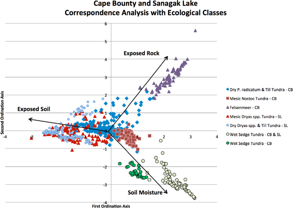
Correspondence analysis results (Table 1) are displayed graphically as a biplot of sample sites arranged on unitless ordination axes (Figure 2). Supplementary environmental variables that were collected in the field, such as soil moisture; exposed rock and soil are not used during the derivation of the ordination but can be projected passively onto the biplot ordination. These variables do not contribute to the calculation of the ordination results, but their meaning is interpreted using those results [59].
Thomas et al., [15] used the first and second axes for clustering. However, upon examining the biplots and eigenvalues, the authors indicated that these two axes might not adequately represent the relationship between sites. In our analyses, with the variance of the fourth axis explaining >5%, it was decided the site scores from all four ordination axes would be suited as input values for the clustering algorithm. With each sample assigned a cluster, based on its CS site score, MRPP was then used to determine the similarity of the clusters and to decide which should be merged. All the clusters were tested to determine if the null hypothesis (i.e., that there is no difference between the clusters) could be rejected. The null hypothesis was rejected since the groups occupy different regions of species space, as shown by the strong chance corrected within-group agreement (A = 0.44) and test statistics (T = −285.21) (p < 0.005).
MRPP pair-wise comparisons were performed on the original ten clusters to examine similarities in composition. The average T-score for the pair-wise comparisons was −82.3. Clusters 6 and 7 (T = −10.0, A = 0.02) and 8 and 9 (T = −5.8, A = 0.02) were combined and then identified by the lower group number (i.e., 6 and 8) (Table 2). To provide further ecological meaning, gravimetric soil moisture values and total PVC values are presented as the average of all the sample points within a cluster. Visual examination of the biplot does not reveal if similar communities exist at both sites even though soil moisture, exposed rock, and soil exposure appear to be strong environmental factors. When the four axes of the biplot were clustered, the results demonstrate that there was very little mixing of samples from the two study sites within the clusters, indicating the species compositions at each study site are relatively distinct. Figure 3 provides a representation of the clustering dendrogram of all the sites; the clusters are in their correct position but the clustering distances are not to scale.
Clusters 1 and 2 are comprised of the CB sample sites and have similar primary and secondary cover types; till (75.4% and 40.6%) and mosses (8.8% and 27.8%), though in differing proportions. The average PVC for clusters 1 and 2 are 25.4% and 73.4% respectively. In terms of soil moisture each is dry during the peak growing season (13.4% and 20.6% soil moisture for clusters 1 and 2 respectively). Indicator species analysis is applied to aid in cluster identification. The indicator species for cluster 1 is Papaver radicatum (Arctic Poppy) (IV = 42.2) with till (IV = 38.1). Cluster 2 has lichens as the highest indicator species (i.e., Thamnolia subliformis (Worm Lichen) (IV = 31.8) and Cetraria nivalis (Snow Lichen) (IV = 20.7)). Cluster 3 is mesic with average soil moisture of 37.3%. Nostoc commune, a nitrogen fixing cyanobacteria that forms a black crust on the soil [60], is the primary cover (48.6%) and indicator species (IV = 49.0), whereas Salix arctica (IV = 29.8) is the secondary indicator species for cluster 3. With undisturbed soil covered by Nostoc commune, the PVC for the cluster is high at 101.7%. The sites for this cluster are exclusively at CB. When examining the dendrogram, clusters 2 and 3 are more similar to each other than to cluster 1; a result of the lack of vegetation cover in cluster 1. Cluster 4 is dominated by Felsenmeer (68.8%) and mosses (22.1%) and is only found at CB and is very different from the other clusters. The primary indicator species is the lichen Rock Tripe (Umbilicaria spp.) (IV = 91.3).
Dryas spp. is found in the majority of SL sites but rarely at CB; this appears to be the reason for the split of clusters 5 and 6 from the previous clusters. For cluster 5, Dryas spp. is the primary cover (46.0%) and the best indicator species (IV = 38.6). Soil moisture and PVC appear to be the primary difference between clusters 5 and 6. The soil moisture of cluster 5 is 41.2% with PVC of 80.4% while cluster 6 is dry (17.2% soil moisture) and poorly vegetated (i.e., 30.4% PVC). There was no strong indicator species for cluster 5; the primary and secondary covers were till (60.5%) and Dryas spp. (18.4%) respectively.
Clusters 8 and 10 represent the first split in the dendrogram indicating that they are distinct from the other clusters. Cluster 8 was comprised of wetland sites from CB and SL, the only cluster to contain sites from both locations. The species with the highest IV’s for that cluster were Eriophorum spp. (IV = 98.1) and Sphagnum spp. (IV = 36.0). This cluster had saturated soils (123.9%) and a high percentage of vegetation cover (154.0%). Cluster 10 sites were only located at SL; they were slightly drier (83.3%) and with slightly less PVC (139.6%). The primary difference between cluster 8 and cluster 10 is the presence of Dryas spp. (42.7%) in cluster 10 sites.
The SSA for the combined dataset of the CB and SL indicated clusters 1 and 2 (which were comprised solely of the CB sites) be combined (J-M = 0.6). For SL, clusters 8 and 10 had poor spectral separability (J-M = 0.83) and were combined to form a single cluster. Clusters 5 and 6 had a weak separability measure (J-M = 1.23) but were left as separate classes due to their differences in soil moisture (41.2% vs. 17.2%) and PVC (80.4% vs. 30.4%). Both classes had Dryas spp. as a major cover type (46.0% and 18.4%) but differing proportions. Clusters 5, 6 and a combination of 8 and 10 form the three ecological classes for the SL component of the combined CA (Table 2).
3.2. Ecological Classifications
Maximum likelihood classifications of the ecological classes derived from the correspondence analysis, clustering, and signature separability for CB and SL show moderate classification results (Figures 4 and 5). The overall accuracy of the CB classification was 79.1% with a kappa coefficient of 0.69 (Table 3). Dry P. radicatum and Till Tundra and Mesic Nostoc Tundra had the highest errors of omission (37%) and commission (46%) respectively. In other words, 37% of the validation sites for Dry P. radicatum and Till Tundra were spectrally similar to another class, primarily Mesic Nostoc Tundra class (15.7%). While 46% of the classified Mesic Nostoc Tundra image pixels spectrally aligned with that class the samples had species compositions similar to other classes. On the CA biplot, Mesic Nostoc Tundra is central to all of the other classes suggesting that it may be a gradient community and share species and ecological characteristics of the other sites. The fewest classification errors occurred between the Felsenmeer class and Wet Sedge Tundra, each of which possessed clearly defined clusters in ordination space.
The classification for SL (Figure 5) showed slightly poorer results than those for CB, with an overall accuracy of 69.2% with a kappa coefficient of 0.54 (Table 4). The majority of the classification errors of commission and omission occurred with Mesic Dryas spp. Tundra classes (34% and 45% respectively). When examining the biplot, the Dryas spp. Tundra classes overlap; the species combinations of these two classes are similar, with the primary difference being an increase in cover of Dryas spp. as you move along the ordination axis. The result is that these classes are spectrally similar and generating errors in the classifications. Thomas et al.[15] noted a similar problem with the classification of a peatland using CA ordination in that it can be difficult to discriminate class boundaries along a latent environmental gradient because of spectral similarities.
4. Discussion
4.1. Ecological Classes
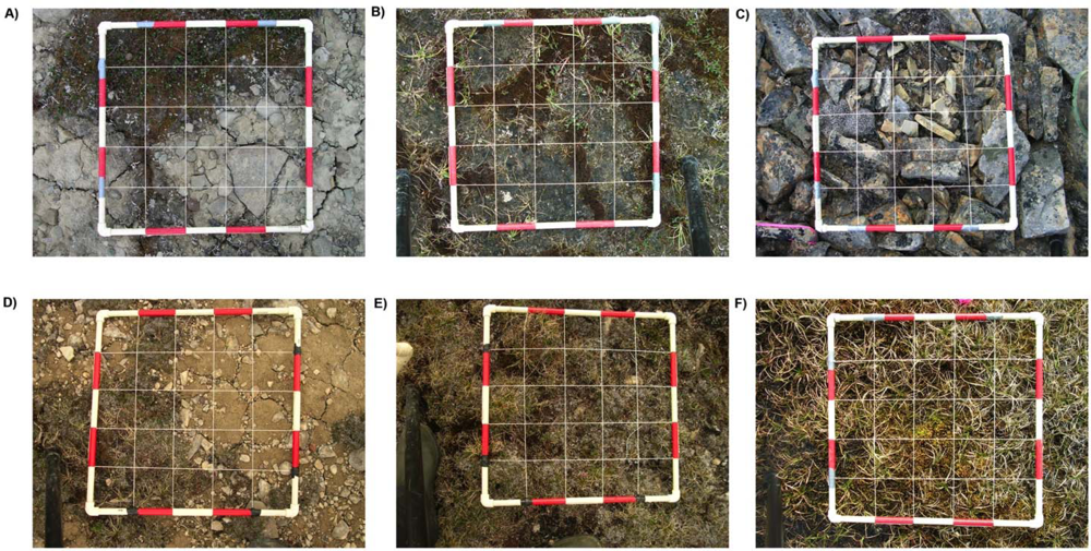
The final classification scheme has been derived based on soil moisture preferences and indicator species. To aid in interpretation and to link the larger-scale CAVM classifications with the classes that have been created here, the bioclimatic classification identifier has also been included (Table 2). By examining the CA biplots of sample sites, which are separated into their ecological classifications, and with supplementary environmental variables overlain, the underlying latent variables can be interpreted to better understand the ecological classifications that have been created [59]. It is illustrated in Figure 6 that the supplementary variables are strongly correlated with the arrangement of the sample sites in ordination space. For example, the Felsenmeer class (Figure 7(c)), that was only present at CB, is distinctly clustered in the upper right quadrant of the biplot. These sites are located at CB on steep slopes and ridge tops where the sloping sedimentary bedrock is relatively close to the surface and has been frost shattered.
Classes at CB and SL align themselves along a gradient of the first ordination axis. Dry and Mesic Dryas spp. Tundra classes (Figure 7(d,e)) of SL are further down the first ordination axis followed by the Dry P. radicatum and Till Tundra (Figure 7(a)) and Mesic Nostoc Tundra (Figure 7(b)) of CB. Though this gradient is aligned with the supplementary variable of exposed soil, it may illustrate that there may be other latent environmental variables, at both sites, that may be impacting species compositions and abundances for these classes. Primary production in arctic vegetation communities is limited by climatic conditions and nutrient supply [60,61]. The amount of available nitrogen, in the form of ammonium (NH4+) and/or nitrate (NO3−), is one of the major factors limiting plant growth in the Arctic [62–64]. The main input of nitrogen originates from biological nitrogen fixation by cyanobacteria, such as Nostoc commune[65–67]. For the study area at SL, over 25% of the Mesic Dryas spp. Tundra sites contain Nostoc commune whereas it was only found in 11% of the Dry Dryas spp. Tundra sites. The increase in available nitrogen may result in the increase in vegetation cover for these sites.
The individual classes of each site also follow a soil moisture gradient. Dry P. radicatum and Till Tundra at CB and Dry Dryas spp. and Till Tundra at SL are most closely classified as P1—Prostrate dwarf-shrub, herb tundra. This is dry patchy tundra with graminoids and forbs being dominant [3]. At both sites micro-scale topographic features (e.g., frost cracks) create moisture gradients that influence the pattern and distribution of vegetation [42]. Plant growth is limited to frost cracks and depressions where wind speeds are reduced, thereby decreasing rates of evaporation and facilitating the accumulation of plant detritus which increases soil moisture and nutrient availability [68]. Clusters 1 and 2, as originally derived, appear to be a sampling artifact in that they are spatially similar except that the quadrats of cluster 1 tend to over-sample dry bare areas while quadrats of cluster 2 tend to over-sample micro-topographic features with higher vegetation and soil moisture. This may also be due to proportional differences between sites. With vegetation limited to small-scale features, the impact on the spectral signature of these plots will often be dominated by the exposed soil due to the spatial resolution of the imagery.
The Mesic Dryas spp. Tundra (G2—Graminoid, prostrate dwarf-shrub, forb tundra) classes of SL and Mesic Nostoc Tundra of CB (G1—Rush/grass, forb, cryptogam tundra) are similar with respect to moisture regime and PVC. The primary difference between the CB and SL sites is the dominance of Dryas spp. at SL; it is found in 82.7% of the samples whereas shrub cover at CB was limited to Salix spp.
The lower right quadrant, strongly associated with moist soils, contains the Wet Sedge Tundra class (Figure 7(f)). This cluster of sample sites contains the CB and SL samples, demonstrating that although they are from distinctly different study sites, the vegetation communities are similar in their composition and dependence on readily available soil moisture. At both CB and SL, Wet Sedge Tundra sites (most closely related to W1—Sedge/grass, moss wetland [3]) are often located in areas with high levels of soil moisture through the growing season, due to proximity of large upslope snow banks. The reason for the creation of an additional wetland class at SL is the presence of Dryas spp. in some of the sample sites.
CB and SL appear to have a natural moisture gradient, at peak season, that generates three distinct moisture categories across the landscape; dry, mesic and wet [11,69,70]. Variations along this gradient may not simply be limited to vegetation composition and structure but extend to ecosystem function and processes; e.g., carbon flux (CO2; CH4) and nitrogen availability/mobilization [7].
4.2. Suitability of the Techniques and Future Development
Based on ordination and clustering of PVC sample data, we were successful in generating meaningful ecological classifications for two separate arctic environments (i.e., SL ∼ 70°N and CB ∼ 75°N). The accuracy results from this methodology may be typically lower than those of traditional a priori image classification techniques. Traditional supervised classification relies solely on user selected spectral training sets to define the image classes. The value of a supervised classification is based only on the validity and usefulness of the a priori classes and the user’s ability to select spectrally distinct training data. In this research the value in the final classes is that they represent distinct species assemblages that relate to environmental variables and are not predetermined or dependant on the user’s ability to select spectral training sets. Though the success of the final classifications was mixed, the methodology identified distinct and similar ecological classes at the two sites based on the species composition and spectral separability, and without a priori classes. Thomas et al.[15] used comparable techniques, showing less favourable results than observed here, albeit for a more “ecologically complex” peatland (i.e., with nine different classes). The improved results observed here may be a function of the reduced complexity of the environment in which this methodology has been applied. In addition, the inclusion of vegetated and non-vegetated ground cover in the analysis, as suggested by Lewis [23], has improved results, specifically for this rather harsh environment. Arctic vegetation communities, particularly in the mid and high arctic, display a patchy collection of discrete communities, often associated with a soil moisture gradient related to topography. For instance, CB is comprised of spatially and spectrally distinct patches, such as Wet Sedge Tundra and Felsenmeer, within a landscape primarily comprised of Dry P. radicatum and Till Tundra (71.6%). Jongman et al.[48] explain that if the vegetation pattern shows distinct groupings of species then classification (clustering) is an appropriate framework for conceptualizing communities; in the case of CB, this appears to have contributed to achieving higher classification accuracies. Unlike CB, SL does not appear to have clear and distinct patches of vegetation. Although distinct patches of Wet Sedge Tundra do exist in the SL study area, it is clear that there is a more gradual change of vegetation cover from the Dry to Mesic Dryas spp. Tundra communities. The spectral similarities of these communities, due to the preponderance of Dryas spp., resulted in reduced classification success. Although two conceptual models exist: (i) the landscape consists of a mosaic of patches; or (ii) the landscape varies continuously along one or more environmental gradients; it appears that the landscape in question may best determine which model to select [9,14]. A potential solution to this may be to incorporate fuzzy classification methods. Rather than creating discrete patches, fuzzy set classifications represent a probability surface and have shown to better reflect the nature of some vegetation gradients [71]. Additionally, for this study, only the original four multispectral bands were included in the image classification. Simple transformations of band reflectance have been shown, for a range of vegetation communities, to be closely correlated with plant biophysical qualities [19]. The normalized difference vegetation index (NDVI) has been shown to have correlations to AGB and PVC [1,13,21,42,73]. Spectral vegetation indices such as NDVI could be included in the image classification procedure to incorporate spectral biophysical derivatives such as AGB.
The benefit of CA in this research, where there was a lack of environmental field data, is that sample sites are organized based on theoretical variables that best explain the greatest variation allowing for the identification of those variables. Supplementary environmental variables that were collected in the field, such as soil moisture, exposed rock, and exposed soil can be projected passively onto the biplot of ordination space to aid in the interpretation of the environmental variables affecting species and abundance. Although the vegetation communities identified appear to have a strong correspondence to soil moisture and exposed rock, there also appears to be some underlying variables such as nutrient availability and/or soil pH. The relationships observed with soil moisture concur with the bioclimatic zones and community classifications described by Walker et al.[3]. Though the classes generated by Walker et al.[3] are general and are applied at a very coarse scale, they do appear to relate to the finer scale ecological classes derived in this study. Inclusion of additional environmental data, such as soil pH, NH4+ and NO3− concentrations, may assist in the understanding/explanation of anomalies observed with respect to latent environmental variables.
Other ordination techniques, such as canonical correspondence analysis (CCA) select the linear combination of measured environmental variables that maximize the dispersion of the species scores [48]. CCA is a ‘restricted correspondence analysis’ in the sense that the site and species scores are restricted to a linear combination of measured variables giving rise to as many axes as there are environmental variables. The inclusion of additional environmental variables and CCA may create more distinct clusters in species space, thereby improving the separation of ecological classes. Additionally, ecological classes derived from the use of CCA would have defined environmental values as opposed to ‘latent’ associations.
The hypothesis that was tested in this research was that: Spectrally distinct vegetation classes that relate to important underlying environmental variables can be created using a combination of ecological and remote sensing techniques for disparate high- and mid-arctic tundra research sites. Unfortunately, this hypothesis does not hold true for both study sites. At CB, where a mosaic of patches was clear and distinct, this hypothesis can be confirmed, whereas at SL, with the exception of the Wet Sedge Tundra, this hypothesis is refuted. At SL there was difficulty in distinguishing between the Dry and Mesic Dryas spp. classes due to the variation in cover along an underlying environmental gradient. The inclusion of additional measured environmental variables and the use of CCA may improve these results. Overall, this research does create meaningful vegetation classifications that relate to underlying ecological processes. The methodology described for the creation of these classification may be useful in developing a better understanding of GEP and ER since both can be related to factors such as vegetation cover, soil moisture, N availability, and micro topography [6,72].
4. Conclusions
The results of this study illustrate that a combination of ecological and remote sensing techniques can produce image classifications that are ecologically meaningful and spectrally significant in a high Arctic environment without a priori classes. The combination of correspondence analysis (CA), clustering and multi-response permutation procedure (MRPP) techniques in conjunction with remote sensing techniques such as spectral separability analysis (SSA) to create ecological classes for use as calibration data can create ecologically meaningful classifications of vegetation communities. The results demonstrate that the incorporation of species abundance data for ecological ordination/clustering can assist in the spectral classification of Arctic environments when using high spatial resolution data. Classification results (overall accuracies between 69% to 79% and Kappa values of 0.54–0.69) may be considered low when compared to traditional supervised and unsupervised classification techniques, but the resulting classifications provide greater ecological meaning in Arctic environments. Difficulties in delineating some ecological classes may be improved with the inclusion of additional environmental variables, such as soil pH and nutrient data (e.g., ammonium (NH4+) and nitrate (NO3−)) and the application of canonical correspondence analysis.
Understanding the spatial relationship between environmental variables and the associated vegetation patterns will provide insight into the structure and function of arctic vegetation communities. This may lead to more informed predictions of the impact of a warming climate on vegetation productivity and ecosystem function. The creation of spectrally distinct, statistically derived ecological classifications may prove extremely useful for monitoring vegetation patterns and processes, and as such, can be utilized to predict patterns of carbon dioxide exchange.
Acknowledgments
The authors would like to thank Jake Wall, Freyja Forsyth, and Shanley Thompson for their sampling assistance in the field. Thank you goes to Scott Lamoureux, Director of the Cape Bounty Arctic Watershed Observatory for his guidance. Thank you to Andrew Millward of Ryerson University for his manuscript review. This work was supported by the Polar Continental Shelf Program and travel assistance was received from the Department of Indian Affairs and Northern Development, Northern Scientific Training Program. Funding was provided by Natural Sciences and Engineering Research Council of Canada (NSERC) in the form of Postgraduate Doctorial Scholarship to David Atkinson and a Discovery Grant to Paul Treitz.
References
- Hope, A.S.; Kimball, J.S.; Stow, D.A. The relationship between tussock tundra spectral reflectance properties and biomass and vegetation composition. Int. J. Remote Sens 1993, 14, 1861–1874. [Google Scholar]
- Stow, D.A.; Hope, A.; McGuire, D.; Verbyla, D.; Gamon, J.; Huemmrich, F.; Houston, S.; Racine, C.; Sturm, M.; Tape, K.; et al. Remote sensing of vegetation and land-cover change in Arctic tundra ecosystems. Remote Sens. Environ 2004, 89, 281–308. [Google Scholar]
- Walker, D.A.; Raynolds, M.K.; Daniels, F.J.A.; Einarsson, E.; Elvebakk, A.; Gould, W.A.; Katenin, A.E.; Kholod, S.S.; Markon, C.J.; Melnikov, E.S.; et al. The circumpolar arctic vegetation map. J. Veg. Sci 2005, 16, 267–282. [Google Scholar]
- Intergovernmental Channel on Climate Change (IPCC). Working Group I: The Physical Science Basis of Climate Change. ARA 4 Report, Observations 4: Changes in Snow, Ice and Frozen Ground. 2007. Available online: http://ipcc-wg1.ucar.edu/wg1/wg1-report.html (accessed on 1 September 2012).
- ACIA. Arctic Climate Impact Assessment; Cambridge University Press: Cambridge, UK, 2005. [Google Scholar]
- Shaver, G.R.; Street, L.E.; Rastetter, E.B.; Van Wijk, M.T.; Williams, M. Functional convergence in regulation of net CO2 in heterogeneous tundra landscapes in Alaska and Sweden. J. Ecol 2007, 95, 802–817. [Google Scholar]
- Dagg, J.; Lafleur, P. Vegetation community, foliar nitrogen, and temperature effects on Tundra CO2 exchange across a soil moisture gradient. Arct. Antarc. Alpine Res 2011, 43, 189–197. [Google Scholar]
- Ostendorf, B.; Reynolds, J.F. A model of arctic tundra vegetation derived from topographic gradients. Landscape Ecol 1998, 13, 187–201. [Google Scholar]
- Goetz, S.J.; Prince, S.D. Modeling terrestrial carbon exchange and storage: Evidence and implications of functional convergence in light-use efficiency. Adv. Ecol. Res 1999, 28, 57–92. [Google Scholar]
- McMichael, C.E.; Hope, A.S.; Stow, D.A.; Fleming, J.B.; Vourlitis, G.; Oechel, W. Estimating CO2 exchange at two sites in Arctic tundra ecosystems during the growing season using a spectral vegetation index. Int. J. Remote Sens 1999, 20, 683–698. [Google Scholar]
- Nobrega, S.; Grogan, P. Landscape and ecosystem-level controls on net carbon dioxide exchange along a natural moisture gradient in Canadian low arctic tundra. Ecosystems 2008, 11, 377–396. [Google Scholar]
- Braun-Blanquet, J. Plant Sociology: The Study of Plant Communities; Mcgraw-Hill: New York, NY, USA, 1965. [Google Scholar]
- Boelman, N.T.; Stieglitz, M.; Rueth, H.M.; Sommerkorn, M.; Griffin, K.L.; Shaver, G.R. Response of NDVI, biomass, and ecosystem gas exchange to long-term warming and fertilization in wet sedge tundra. Oecologia 2003, 135, 414–421. [Google Scholar]
- Williams, M.; Rastetter, E.B.; Shaver, G.R.; Hobbie, J.E.; Carpino, E.; Kwiatkowski, B.L. Primary production in an arctic watershed: An uncertainty analysis. Ecol. Appl 2001, 11, 1800–1816. [Google Scholar]
- Thomas, V.; Treitz, P.M.; Jelinski, D.; Miller, J.; Lafleur, P.; McCaughey, H. Image classification of a northern peatland complex using spectral and plant community data. Remote Sens. Environ 2002, 84, 83–99. [Google Scholar]
- Tieszen, L.L.; Reed, B.C.; Bliss, N.B.; Wylie, B.K.; Dejong, D.D. NDVI C3 and C4 production and distributions in Great Plains grassland land cover classes. Ecol. Appl 1997, 7, 59–78. [Google Scholar]
- Stow, D.A.; Hope, A.S.; Boynton, W.; Phinn, S.; Walker, D.; Auerbach, N.A. Satellite-derived vegetation index and cover type maps for estimating carbon dioxide flux for arctic tundra regions. Geomorphology 1998, 21, 313–327. [Google Scholar]
- Stow, D.A.; Daeschner, S.; Boynton, W.; Hope, A.S. Arctic tundra functional types by classification of single-date and AVHRR bi-weekly NDVI composite datasets. Int. J. Remote Sens 2000, 21, 1773–1779. [Google Scholar]
- Laidler, G.J.; Treitz, P. Biophysical remote sensing of arctic environments. Progr. Phys. Geogr 2003, 27, 44–68. [Google Scholar]
- Stow, D.A.; Burns, B.H.; Hope, A.S. Spectral spatial and temporal characteristics of arctic tundra reflectance. Int. J. Remote Sens 1993, 14, 2445–2462. [Google Scholar]
- Shippert, M.M.; Walker, D.A.; Auerbach, N.A.; Lewis, B.E. Biomass and leaf-area index maps derived from SPOT images for Toolik Lake and Imnavait Creek areas Alaska. Polar Rec 1995, 31, 147–154. [Google Scholar]
- Gould, W.A. Remote sensing of vegetation plant species richness and regional biodiversity hotspots. Ecol. Appl 2000, 10, 1861–1870. [Google Scholar]
- Lewis, M.M. Numeric classification as an aid to spectral mapping of vegetation communities. Plant Ecol 1998, 136, 133–149. [Google Scholar]
- Graetz, R.D. Remote Sensing of Terrestrial Ecosystem Structure: An Ecologist’s Pragmatic View. In Remote Sensing of Biosphere Function; Mooney, HA, Hobbs, RJ, Eds.; Springer-Verlag: New York, NY, USA, 1989; pp. 5–30. [Google Scholar]
- Roughgarden, J.; Running, S.W.; Matson, P.A. What does remote sensing do for Ecology? Ecology 1991, 72, 1918–1922. [Google Scholar]
- Wickland, D.E. Mission to planet earth: The ecological perspective. Ecology 1991, 72, 1923–1933. [Google Scholar]
- Ustin, S.L.; Adams, J.B.; Elvidge, C.D.; Rejmanek, M.; Rock, B.N.; Smith, M.O.; Thomas, R.W.; Woodward, R.A. Thematic mapper studies of semiarid shrub communities. BioScience 1986, 36, 446–452. [Google Scholar]
- Pando, M.; Lange, R.T.; Sparrow, A.D. Relations between reflectance in Landsat MSS wavebands and floristic composition of Australian chenopod rangelands. Int. J. Remote Sens 1992, 13, 1861–1867. [Google Scholar]
- Hobbs, R.J.; Wallace, J.F.; Campbell, N.A. Classification of vegetation in the Western Australian wheatbelt using Landsat MSS data. Vegetatio 1989, 80, 91–105. [Google Scholar]
- Ghitter, G.S.; Hall, R.J.; Franklin, S.E. Variability of Landsat Thematic Mapper data in boreal deciduous and mixedwood stands with conifer understorey. Int. J. Remote Sens 1995, 16, 2989–3002. [Google Scholar]
- Brook, R.K.; Kenkel, N.C. A multivariate approach to vegetation mapping of Manitoba’s Hudson Bay Lowlands. Int. J. Remote Sens 2002, 23, 4761–4776. [Google Scholar]
- Price, K.P.; Pyke, D.A.; Mendes, L. Shrub dieback in a semiarid ecosystem: The integration of remote sensing and geographic information systems for detecting vegetation change. Photogramm. Eng. Remote Sensing 1992, 58, 455–463. [Google Scholar]
- Catt, P.; Lange, R.T.; Sparrow, A.D. The Botanical and Spectral Separability of Arid Zone Rangeland Plant Communities on Landsat MSS Imagery: A Pilot Study in South Australia. Proceedings of Fourth Australasian Remote Sensing Conference, Adelaide, Australia, August 1987; 1, pp. 145–150.
- Toth, T.; Csillag, F.; Biehl, L.L.; Micheli, E. Characterisation of semi-vegetated salt-affected soils by means of field remote sensing. Remote Sens. Environ 1991, 37, 167–180. [Google Scholar]
- Lewis, M.M. Species composition related to spectral classification in an Australian hummock grassland. Int. J. Remote Sens 1994, 15, 3223–3239. [Google Scholar]
- Treitz, P.M.; Howarth, P.J.; Suffling, R.C.; Smith, P. Application of detailed ground information to vegetation mapping with high spatial resolution digital imagery. Remote Sens. Environ 1992, 42, 65–82. [Google Scholar]
- Jacobsen, A.; Nielson, A.A.; Ejrnaes, R.; Groom, G.B. Spectral identification of Danish grassland classes related to management and plant species composition. Proceedings of 4th International Airborne Remote Sensing Conference and Exhibition/21st Canadian Symposium On Remote Sensing, Ottawa, ON, Canada, 21–24 June 1999; 1, pp. 74–81.
- Anderson, M.J.; Clements, A. Resolving environmental disputes: a statistical method for choosing among competing cluster models. Ecol. Appl 2000, 10, 1341–1355. [Google Scholar]
- Hodgson, D.A.; Vincent, J.S.; Fyles, J.G. Quaternary Geology of Central Melville Island Northwest Territories; No 83–16; Geological Survey of Canada: Ottawa, ON, Canada, 1984. [Google Scholar]
- Billings, W.D. Arctic and alpine vegetation: similarities differences and susceptibility to disturbances. BioScience 1973, 23, 685–696. [Google Scholar]
- Walker, D.A.; Gould, W.A.; Maier, H.A.; Raynolds, M.K. The circumpolar arctic vegetation map: AVHRR-derived base maps environmental controls and integrated mapping procedures. Int. J. Remote Sens 2002, 23, 4551–4570. [Google Scholar]
- Laidler, G.J.; Treitz, P.M.; Atkinson, D.M. Remote Sensing of Arctic Vegetation: The relations between NDVI, spatial resolution, and vegetation cover on Boothia Peninsula, Nunavut. Arctic 2008, 61, 1–13. [Google Scholar]
- Wein, R.C.; Rencz, A.N. Plant cover and standing crop-sampling procedures for the Canadian high arctic. Arct. Alp. Res 1976, 8, 139–150. [Google Scholar]
- Chapin, F.S.; Bret-Harte, M.S.; Hobbie, S.E.; Zhong, H. Plant functional types as predictors of transient responses of arctic vegetation to global change. J. Veg. Sci 1996, 7, 347–358. [Google Scholar]
- Norum, R.A.; Miller, M. Gen. Tech. Rep. PNW-171: Measuring Fuel Moisture Content in Alaska: Standard Methods and Procedures; US Department of Agriculture, Forest Service Pacific Northwest Forest and Range Experiment Station: Portland, OR, USA, 1984. [Google Scholar]
- NASA (National Aeronautics and Space Administration). Landsat 7 Science Data User’s Handbook. 2002. Available online: http://landsathandbook.gsfc.nasa.gov (accessed on 31 August 2012).
- Taylor, M. IKONOS Planetary Reflectance and Mean Solar Exo-Atmospheric Irradiance. In IKONOS Planetary Reflectance QSOL Rev.1; Space Imaging Inc. (now GEOEYE Inc.): Herndon, VA, USA, 2005. [Google Scholar]
- Jongman, R.H.G.; ter Braak, C.J.F.; van Tongeren, O.F.R. (Eds.) Data Analysis in Community and Landscape Ecology; Cambridge University Press: Cambridge, UK, 1995.
- McCune, B.; Grace, J.B. Analysis of Ecological Communities; MJM Software Design: Gleneden Beach, OR, USA, 2002. [Google Scholar]
- Cumming, B. Personal Communication. Department of Biology, Queen’s University, Kingston, ON, Canada,. 2007.
- Equihua, M. Fuzzy clustering of ecological data. J. Ecol 1990, 78, 519–534. [Google Scholar]
- Nekola, J. Vascular plant compositional gradients within and between Iowa fens. J. Veg. Sci 2004, 15, 771–780. [Google Scholar]
- Ward, J.H. Hierarchical grouping to optimise an objective function. J. Amer. Stat Assoc 1963, 58, 236–244. [Google Scholar]
- Causton, D.R. An Introduction to Vegetation Analysis: Principles Practice and Interpretation; Unwin Hyman: Boston, MA, USA, 1988. [Google Scholar]
- Jensen, J.R. Introductory Digital Image Processing: A Remote Sensing Perspective, 3rd ed; Prentice Hall: Englewood Cliffs, NJ, USA, 2005. [Google Scholar]
- Bruzzone, L.; Roli, F.; Serpico, B. An extension of the Jeffreys-Matusita Distance to Multiclass Cases for feature selection. IEEE Trans. Geosci. Remote Sens 1995, 6, 1318–1321. [Google Scholar]
- Schott, J.R. Remote Sensing: The Image Chain Approach; Oxford Univ Press: Toronto, ON, Canada, 1997. [Google Scholar]
- Dufrene, M.; Legendre, P. Species assemblages and indicator species: the need for a flexible asymmetrical approach. Ecol. Monogr 1997, 67, 345–366. [Google Scholar]
- Lepš, J.; Šmilauer, P. Multivariate Analysis of Ecological Data Using CANOCO; Cambridge University Press: Cambridge, UK, 2003. [Google Scholar]
- Liengen, T.; Olsen, R. Nitrogen fixation by free-living cyanobacteria from different coastal sites in a high arctic tundra, Spitsbergen. Arct. Alp. Res 1997, 29, 470–477. [Google Scholar]
- Dickson, L.G. Constraints to nitrogen fixation by cryptogamic crusts in a polar desert ecosystem, Devon Island, NWT, Canada. Arct. Antarct. Alpine Res 2000, 32, 40–45. [Google Scholar]
- Shaver, G.R.; Chapin, F.S. Response to fertilization by various plant growth forms in an Alaskan tundra. Ecology 1980, 61, 662–675. [Google Scholar]
- Nadelhoffer, K.J.; Giblin, A.E.; Shaver, G.R.; Lirikins, A.E. Microbial Processes and Plant Nutrient Availability in Arctic Soils. In Arctic Ecosystems in a Changing Climate: An Ecophysiological Perspective; Chapin, F.S., III, Jefferies, R.L., Reynolds, J.F., Shaver, G.R., Svoboda, J., Eds.; Academic Press Inc: San Diego, CA, USA, 1992; pp. 281–300. [Google Scholar]
- Atkin, O.K. Reassessing the nitrogen relations of Arctic plants: A mini-review. Plant Cell Environ 1996, 19, 695–704. [Google Scholar]
- Alexander, V. A Synthesis of the IBP Tundra Biome Study of Nitrogen Fixation. In Soil Organisms and Decomposition in Tundra; Holding, A.J., Heal, O.W., MacLean, S.F., Flanagan, P.W., Eds.; Tundra Biome Steering Committee: Stockholm, Sweden, 1974; pp. 109–121. [Google Scholar]
- Lennihan, R.; Chapin, D.M.; Dickson, L.G. Nitrogen fixation and photosynthesis in high arctic forms of Nostoc commune. Can. J. Bot 1994, 72, 940–945. [Google Scholar]
- Solheim, B.; Endal, A.; Vigstad, H. Nitrogen fixation in Arctic vegetation and soils from Svalbard, Norway. Polar Biol 1996, 16, 35–40. [Google Scholar]
- Oberbauer, S.F.; Dawson, T.E. Water-Relations of Arctic Vascular Plants. In Arctic Ecosystems in a Changing Climate—An Ecophysiological Perspective; Chapin, S.F., III, Jefferies, R.L., Reynolds, J.F., Shaver, G.R., Svoboda, J., Chu, E.W., Eds.; Academic Press Inc.: San Diego, CA, USA, 1992; pp. 259–279. [Google Scholar]
- Bliss, L.C.; Matveyeva, N.V. Circumpolar Arctic Vegetation. In Arctic Ecosystems in a Changing Climate—An Ecophysiological Perspective; Chapin, S.F., III, Jefferies, R.L., Reynolds, J.F., Shaver, G.R., Svoboda, J., Chu, E.W., Eds.; Academic Press Inc.: San Diego, CA, USA, 1992; pp. 59–89. [Google Scholar]
- Walker, D.A. Hierarchical subdivision of arctic tundra based on vegetation response to climate, parent material, and topography. Global Change Biol 2000, 6, 9–34. [Google Scholar]
- Foody, G.M. Approaches for the production and evaluation of fuzzy land cover classifications from remotely sensed data. Int. J. Remote Sens 1996, 17, 1317–1340. [Google Scholar]
- Walker, D.A.; Epstein, H.E.; Jia, G.J.; Balser, A.; Copass, C.; Edwards, E.J.; Gould, W.A.; Hollingsworth, J.; Knudson, J.; Maier, H.A.; et al. Phytomass, LAI, and NDVI in northern Alaska: Relationships to summer warmth, soil pH, plant function types, and extrapolation to the circumpolar arctic. J. Geophys. Res 2003, 108, D2. [Google Scholar]
Figure 1.
The study areas of: (A) Cape Bounty, Melville Island, Nunavut; and (B) Sanagak Lake, Boothia Peninsula, Nunavut. IKONOS imagery is displayed as a colour infrared composite image with Bands 4, 3, 2.
Figure 1.
The study areas of: (A) Cape Bounty, Melville Island, Nunavut; and (B) Sanagak Lake, Boothia Peninsula, Nunavut. IKONOS imagery is displayed as a colour infrared composite image with Bands 4, 3, 2.
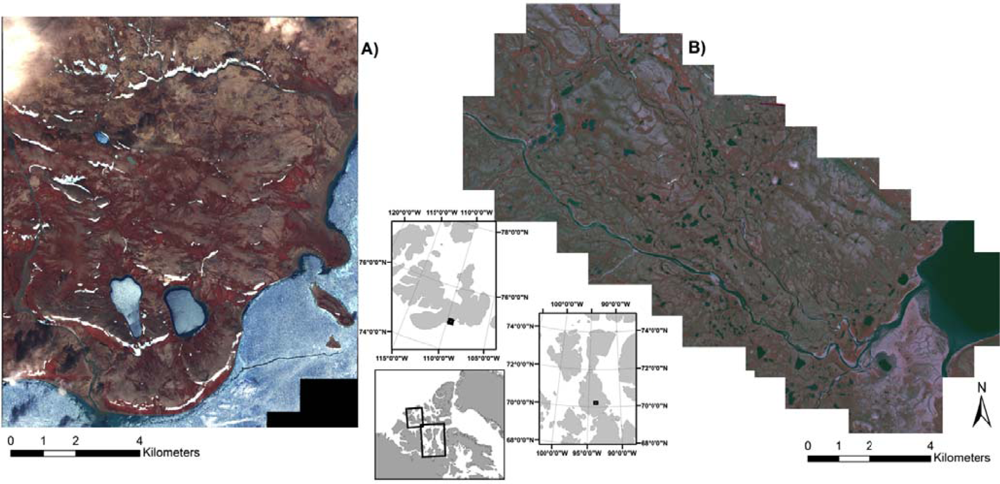
Figure 2.
The CA biplot of the combined dataset of CB and SL with the first and second ordination axes and supplementary environmental variables overlain to aid in interpretation (soil moisture, exposed rock, exposed soil).
Figure 2.
The CA biplot of the combined dataset of CB and SL with the first and second ordination axes and supplementary environmental variables overlain to aid in interpretation (soil moisture, exposed rock, exposed soil).
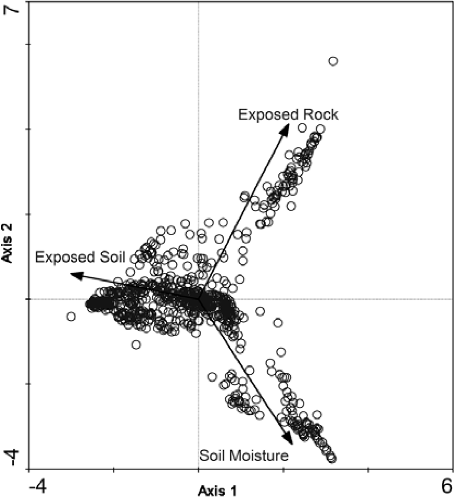
Figure 3.
Dendrogram of the combined dataset of CB and SL samples post Multi-Response Permutation Procedures (MRPP) analysis but prior to Spectral Separability Analysis (SSA), generated 10 vegetation classes. Classes 1–4 were unique to CB, while 5, 6, and 10 were unique to SL. Only class 8 had shared samples from both sites.
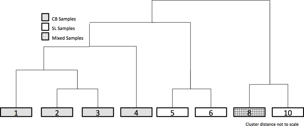
Figure 4.
Cape Bounty CA ecological classification.
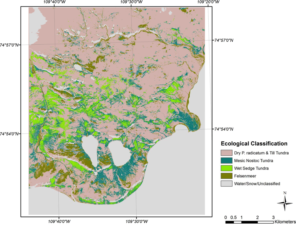
Figure 5.
Sanagak Lake CA ecological classification.
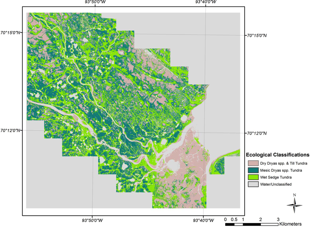
Figure 6.
CA biplot with supplementary environmental variables and ecological class clusters.

Figure 7.
Representative images of the final ecological classes. (A) Dry P. radicatum and Till Tundra; (B) Mesic Nostoc Tundra; (C) Felsenmeer; (D) Dry Dryas spp. and Till Tundra; (E) Mesic Dryas spp. Tundra; and (E) Wet Sedge Tundra.
Figure 7.
Representative images of the final ecological classes. (A) Dry P. radicatum and Till Tundra; (B) Mesic Nostoc Tundra; (C) Felsenmeer; (D) Dry Dryas spp. and Till Tundra; (E) Mesic Dryas spp. Tundra; and (E) Wet Sedge Tundra.

Table 1.
Correspondence Analysis (CA) results for the combined datasets of Cape Bounty (CB) and Sanagak Lake (SL).
| CA Axis | 1 | 2 | 3 | 4 | Sum | Total Eigenvalue |
|---|---|---|---|---|---|---|
| Eigenvalue | 0.5 | 0.45 | 0.34 | 0.22 | 1.51 | 3.14 |
| % Variance | 16 | 14.4 | 10.9 | 7 | 48.3 |
| CB and SL CA | 1 | 2 | 3 | 4 | 5 | 6* | 8* | 10 |
| Cluster | ||||||||
| % Soil Moisture | 13.4 | 20.6 | 37.3 | 15.9 | 41.2 | 17.2 | 123.9 | 83.3 |
| PVC | 25.4 | 73.4 | 101.7 | 48.0 | 80.4 | 30.4 | 154.0 | 139.6 |
| Primary Cover | Till (75.4%) | Till (40.6%) | Nostoc commune (48.6%) | Rock (68.8%) | Dryas spp. (46.0%) | Till (60.5%) | Sphagnum spp (82.7%) | Sphagnum spp (46.8%) |
| Secondary Cover | Mosses (8.8%) | Mosses (27.8%) | Mosses (32.6%) | Mosses (22.1%) | Carex spp. (10.6%) | Dryas spp. (18.4%) | Eriophorum spp. (60.1%) | Dryas spp. (42.7%) |
| Primary IV | P. radicatu m (42.2) | Thamnolia subliformis (31.8) | Nostoc commune (49.0) | Umbilicari a spp. (91.3) | Dryas spp. (38.6) | n/a | Eriophorum spp. (56.4) | n/a |
| Secondary IV | Till (38.1) | Cetraria nivalis (20.7 ) | Salix arctica (29.8) | Rock (88.3) | Saxifraga oppositifola (17.8) | n/a | Sphagnum spp (31.1) | n/a |
| Majority Sites | Cape Bounty | Cape Bounty | Cape Bounty | Cape Bounty | Sanagak Lake | Sanagak Lake | Mixed | Sanagak Lake |
| CB and SL CA | 1 (Combined Cluster 1 & 2) | 3 | 4 | 5 | 6 | 8 | 10 Combined 8 & 10 (for Sanagak Lake Only) | |
| Final Cluster | ||||||||
| % Soil Moisture | 17.1 | 37.3 | 15.9 | 41.2 | 17.2 | 123.9 | 123.3 | |
| PVC | 50.2 | 101.7 | 48.0 | 80.4 | 30.4 | 154.0 | 144.8 | |
| Primary Cover | Till (57.6%) | Nostoc commune (48.6%) | Rock (68.8%) | Dryas spp. (46.0%) | Till (60.5%) | Sphagnum spp (82.7%) | Sphagnum spp (69.3%) | |
| Secondary Cover | Mosses (18.5%) | Mosses (32.6%) | Mosses (22.1%) | Carex spp. (10.6%) | Dryas spp. (18.4%) | Eriophorum spp. (60.1%) | Eriophorum spp. (47.5%) | |
| Primary IV | P. radicatum (38.4) | Nostoc commune (49.0) | Umbilicari a spp. (91.3) | Dryas spp. (38.6%) | n/a | Eriophorum spp. (56.4) | Eriophorum spp. (43) | |
| Secondary IV | Till (38.0) | Salix arctica (29.8) | Rock (88.3) | Saxifraga oppositifolia (17.8) | n/a | Sphagnum spp (31.1) | Sphagnum spp (27) | |
| Classification | Cape Bounty | Cape Bounty | Cape Bounty | Sanagak Lake | Sanagak Lake | Cape Bounty | Sanagak Lake | |
| Bioclimactic Class | P1 | G1 | n/a | G2 | P1 | W1 | W1 | |
| Ecological Class Name | Dry P. radicatum & Till Tundra | Mesic Nostoc Tundra | Felsenmeer | Mesic Dryas spp. Tundra | Dry Dryas spp. & Till Tundra | Wet Sedge Tundra | Wet Sedge Tundra | |
| Reference Class | # of Pixels | Percent Classified into Class | |||
|---|---|---|---|---|---|
| 1 (Dry P. radicatum & Till Tundra) | 3 (Mesic Nostoc Tundra) | 4 (Felsenmeer) | 8 (Wet Sedge Tundra) | ||
| Unclassified | 2 | 0.22 | 0 | 0 | 0 |
| 1 | 598 | 63.0 | 8.6 | 0 | 1.8 |
| 3 | 406 | 15.7 | 85.9 | 0 | 6.1 |
| 4 | 179 | 6.4 | 0 | 100 | 0 |
| 8 | 858 | 14.7 | 5.5 | 0 | 92.1 |
| Overall Accuracy | 79.1% | ||||
| Kappa Coefficient | 0.69 | ||||
| 95% Confidence Interval | 0.669–0.720 | ||||
| Reference Class | # of Pixels | Percent Classified into Class | |||
|---|---|---|---|---|---|
| 6 (Dry Dryas spp. & Till Tundra) | 5 (Mesic Dryas spp. & Till Tundra) | 10 (Wet Sedge Tundra) | |||
| Unclassified | 18 | 0 | 2.6 | 1.0 | |
| 6 | 523 | 68.9 | 25.5 | 2.6 | |
| 5 | 487 | 28.7 | 55.3 | 0 | |
| 10 | 405 | 2.4 | 16.6 | 96.4 | |
| Overall Accuracy | 69.2% | ||||
| Kappa Coefficient | 0.54 | ||||
| 95% Confidence Interval | 0.509–0.583 | ||||
Share and Cite
MDPI and ACS Style
Atkinson, D.M.; Treitz, P. Arctic Ecological Classifications Derived from Vegetation Community and Satellite Spectral Data. Remote Sens. 2012, 4, 3948-3971. https://doi.org/10.3390/rs4123948
AMA Style
Atkinson DM, Treitz P. Arctic Ecological Classifications Derived from Vegetation Community and Satellite Spectral Data. Remote Sensing. 2012; 4(12):3948-3971. https://doi.org/10.3390/rs4123948
Chicago/Turabian StyleAtkinson, David M., and Paul Treitz. 2012. "Arctic Ecological Classifications Derived from Vegetation Community and Satellite Spectral Data" Remote Sensing 4, no. 12: 3948-3971. https://doi.org/10.3390/rs4123948