SR-4000 and CamCube3.0 Time of Flight (ToF) Cameras: Tests and Comparison

Abstract

In this paper experimental comparisons between two Time-of-Flight (ToF) cameras are reported in order to test their performance and to give some procedures for testing data delivered by this kind of technology. In particular, the SR-4000 camera by Mesa Imaging AG and the CamCube3.0 by PMD Technologies have been evaluated since they have good performances and are well known to researchers dealing with Time-of-Flight (ToF) cameras. After a brief overview of commercial ToF cameras available on the market and the main specifications of the tested devices, two topics are presented in this paper. First, the influence of camera warm-up on distance measurement is analyzed: a warm-up of 40 minutes is suggested to obtain the measurement stability, especially in the case of the CamCube3.0 camera, that exhibits distance measurement variations of several centimeters. Secondly, the variation of distance measurement precision variation over integration time is presented: distance measurement precisions of some millimeters are obtained in both cases. Finally, a comparison between the two cameras based on the experiments and some information about future work on evaluation of sunlight influence on distance measurements are reported.

1. Introduction

In the last few years, a new generation of active sensors has been developed, which allows the acquisition of 3D point clouds without any scanning mechanism and from just one point of view at video frame rates. The working principle is the measurement of the ToF of an emitted signal by the device towards the object to be observed, with the advantage of simultaneously measuring the distance information for each pixel of the camera sensor. Many terms have been used in the literature to indicate these devices, such as: Time-of-Flight (ToF) cameras, Range IMaging (RIM) cameras, 3D range imagers, range cameras or a combination of the mentioned terms. In the following, the term ToF cameras will be employed, because it relates to the working principle of this recent technology.

There are two main approaches currently employed in ToF camera technology: one measures distance by means of direct measurement of the runtime of a travelled light pulse, using for instance arrays of Single-Photon Avalanche Diodes (SPADs) [1,2] or an optical shutter technology [3]; the other method uses amplitude modulated light and obtains distance information by measuring the phase shift between a reference signal and the reflected signal [4]. Such technology is possible because of the miniaturization of semiconductor technology and the evolution of CCD/CMOS processes that can be implemented independently for each pixel. The result is the ability to acquire distance measurements for each pixel at high speed and with accuracies up to 1 cm. While ToF cameras based on the phase shift measurement usually have a working range limited to 10–30 m, cameras based on the direct ToF measurement can measure distances up to 1,500 m (

Table 1. Technical specifications (when available) of Time of Flight (ToF) commercial cameras.

Manufacturer	ToF Camera Model	Working Principle	Max Sensor Resolution [Pixel × Pixel]	Max Range [m]	Focal Distance [m]	Max Framerate [fps]	Signal wavelength [nm]	Default Modulation Frequency [MHz]	Measurement Accuracy/Repeatability (σ)	Weight [kg]
Canesta Inc.	XZ422	Phase shift	160 × 120	n.a.	n.a.	n.a.	n.a.	44	n.a.	n.a.
Canesta Inc.	Cobra	n.a.	320 × 200	n.a.	n.a.	n.a.	n.a.	n.a.	millimetric	n.a.
Fotonic	Fotonic B70	Phase shift	160 × 120	7.0	n.a.	75	808	44	±0.015 m at 3–7 m (accuracy) and ±0.030 m at 3–7 m (uncertainty)	1.049
Mesa Imaging AG	SR-3000	Phase shift	176 × 144	7.5	0.008	25	850	20	n.a.	n.a.
Mesa Imaging AG	SR-4000	Phase shift	176 × 144	5 or 10	0.010	54	850	30 or 15	±0.010 m or ±0.015 m	0.470 - 0.510
Optrima NV	OPTRICAM DS10K-A	Phase shift	120 × 90	10.0	0.0037	50	870	n.a.	noise level <0.03 m at 3.5 m	n.a.
Panasonic	D-Imager (EKL3104)	Phase shift	160 × 120	9.0	n. a.	30	870	n.a.	±0.04 m and σ = 0.03 m (no ambient ill.) or σ = 0.14 m (ambient illum.)	0.52
PMDTechnologies GmbH	PMD19k	Phase shift	160 × 120	7.5	0.012	15	870	20	centimetric	n.a.
PMDTechnologies GmbH	CamCube3.0	Phase shift	200 × 200	7.5	0.013	15	870	21	centimetric	1.438
PMDTechnologies GmbH	A2	Phase shift	64 × 16	9.4–150	n. a.	15	870	16–1	±0.10 m (distance < 40 m)	n.a.
Stanley Electric Ltd.	P-300 TOFCam	Phase shift	128 × 128	15	n. a.	30	850	10	repeatability 1% of the distance (at 3 m)	0.25
Advanced Scientific Concepts Inc.	DRAGONEYE 3D FLASH LIDAR	Direct ToF	128 × 128	1,500	0.017	10	1570	n. a.	±0.10 m and 3σ= ±0.15 m	3
Advanced Scientific Concepts Inc.	TIGEREYE 3D FLASH LIDAR	Direct ToF	128 × 128	60–1,100	n. a.	n. a.	1570	n. a.	±0.04 m at 60 m	1.6 ÷ 2.0
Advanced Scientific Concepts Inc.	PORTABLE 3D FLASH LIDAR	Direct ToF	128 × 128	70–1,100	0.017–0.500	15	1570	n. a.	n. a.	6.5
SoftKinetic	DS311	Direct ToF	160 × 120 + RGB 640 × 480	4.5	n. a.	60	infrared	n. a.	depth resolution <0.03 m at 3 m	n. a.
3DV Systems	ZCamII	Direct ToF (Shutter)	320 × 240 + RGB	10.0	n. a.	n. a.	n. a.	n. a.	n. a.	n. a.
3DV Systems	Zcam	Direct ToF (Shutter)	320 × 240 + RGB 1.3 Mpixel	2.5	n. a.	60	n. a.	n. a.	±0.02 m	0.36

). ToF cameras are usually characterized by low resolution (no more than a few thousands of pixels), small dimensions, costs that are an order of magnitude lower than LiDAR instruments and a lower power consumption with respect to classical laser scanners. In contrast to stereo imaging, the depth accuracy is practically independent of textural appearance, but limited to about 1 cm in the best case (commercial phase shift ToF cameras).

In the last few years, several studies have reported on the performance evaluation and calibration of ToF cameras, with different aims and applications [5–18]. Since this technology has undergone rapid development, different approaches and results have been presented, which are often strictly related to the specific camera model evaluated.

In this paper, comparisons between two recent ToF cameras are presented in order to test their performances and to give some procedures for testing data delivered by this technology. In particular, the SR-4000 camera by Mesa Imaging AG and the CamCube3.0 by PMD Technologies have been tested. Both sensors have good performance and are well known to researchers dealing with ToF cameras. In Section 2, an overview of the main specifications of both cameras is first given. Then, in Section 3 the influence of camera warm up on distance measurement stability is analyzed. In Section 4 the distance measurement precision stability with varying integration time is evaluated for both cameras. Finally, some conclusions and recommendations for future works are presented.

The first prototypes of ToF cameras for civil applications were developed in the late 90s [4]. After many improvements to both sensor resolution and accuracy there are now many commercial ToF cameras available. The main differences between models are related to ranging principle, sensor resolution and measurement accuracy. Table 1 summarizes some technical specifications (when available) about commercial ToF cameras in order to give a general overview of the available products. The column “Measurement accuracy/repeatability” in Table 1 contains heterogeneous information since the camera manufacturers adopt different terms and conditions for this information. It is worth noting the flexibility (and low cost) of the DS311 sensor from SoftKinetic [19] will probably influence the whole market of ToF sensors in the near future.

2. SR-4000 and CamCube3.0 Cameras

As mentioned before, the SR-4000 and the CamCube3.0 cameras have been tested in this work. In Section 2.1, their main specifications are reported while Section 2.2 describes with the output data available with each camera.

2.1. Main Technical Specifications

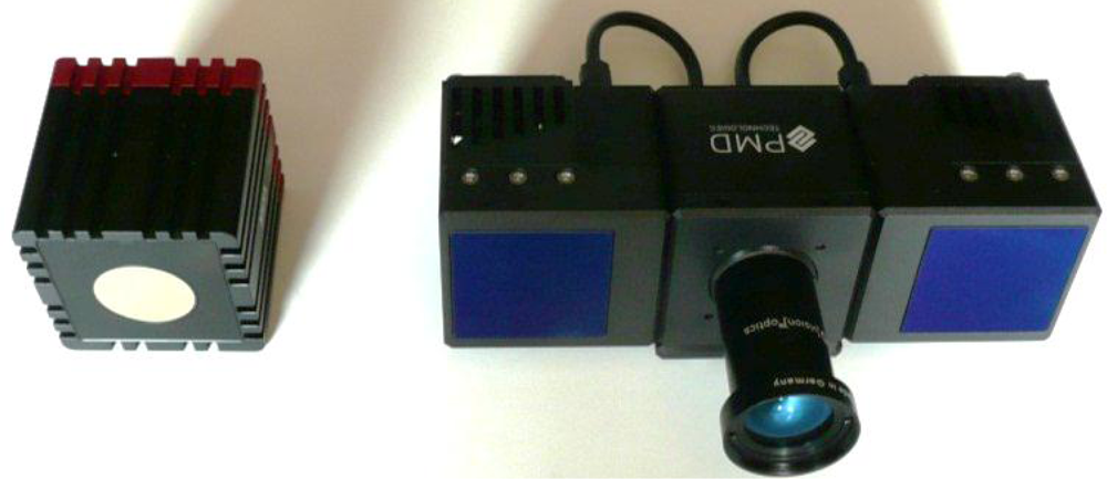
The SR-4000 and the CamCube3.0 cameras are both based on the phase shift measurement principle [4]. The CamCube3.0 has a sensor resolution higher than the SR-4000 one (200 × 200 pixels vs. 144 × 176 pixels), but it is about three times larger and heavier (Figure 1). The SR-4000 distance measurement accuracy is given by the manufacturer as ±0.01 m (30 MHz modulation frequency). This value has been confirmed by experimental tests, such as the ones reported in [17,18]. The distance measurement accuracy of the CamCube3.0 camera is not known, but preliminary tests performed by our group and reported in [16] on the previous model (CamCube2.0) shown a distance measurement accuracy of 3–4 cm. The declared distance measurement repeatability is similar for the two devices (0.004 m for the SR-4000 and 0.003 m for the CamCube3.0), while the working range with standard settings is higher in the case of the PMD camera (0.3–5.0 m for the SR-4000 and 0.3–7.0 m for the CamCube3.0). Mesa Imaging CH also delivers a SR-4000 model with a wider working range (0.3–10.0 m) but a reduce measurement accuracy (±0.015 m) due to the use of a lower modulation frequency (15 MHz).

The declared maximum frame rate of the SR-4000 camera is 54 fps (frames per second) and 40 fps for the CamCube3.0 at full resolution (200 × 200 pixels).

The “crop utility” delivered by PMD allows cropping of pixel columns and rows, therefore it is possible to get a frame rate up to 60 fps considering the same number of pixels of the SR-4000 camera.

Finally, the SR-4000 camera has a passive cooling system, while the CamCube3.0 is equipped with two fans running continuously.

2.2. Output Data

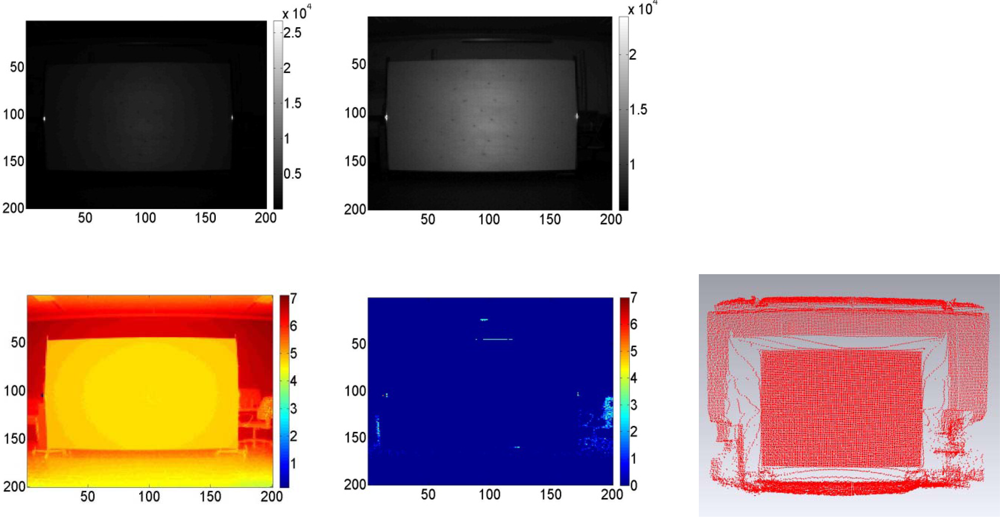
Both cameras deliver a range image and an amplitude image at video frame rates: the range image (or depth image) contains the radial measured distance between the considered pixel and its projection on the observed object, while the amplitude image contains the strength of the reflected signal by the object for each pixel. In the case of the CamCube3.0 an intensity image is also delivered, which represents the mean of the total light incident on the sensor (reflected modulated signal and background light of the observed scene). In both cameras, a confidence map (SR-4000) or a flag matrix (CamCube3.0) is also delivered, which contains information about the quality of the acquired data (i.e., saturated pixels, low signal amplitudes, etc.). Moreover, a 3D point cloud (with X, Y and Z coordinates referred to the local coordinate system of the camera) is also delivered, which is equivalent to a 3D scan from classical LiDAR instruments with the advantage of real time acquisition.

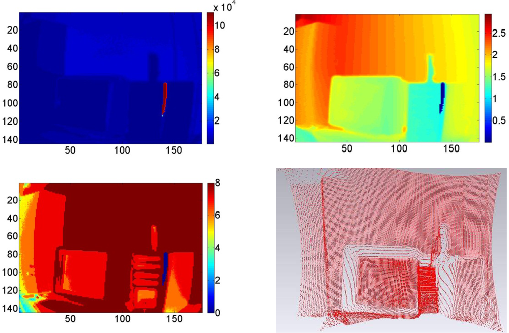
In order to give idea sample of the data acquired with the two tested cameras, some visualizations of data acquired with the SR-4000 and the CamCube3.0 cameras are given in Figures 2 and 3 respectively. It should be noted that the SR-4000 software only returns calibrated (for lens model) data, while the CamCube3.0 software allows the user to access both raw and calibrated data.

3. Warm-Up Period Evaluation

Since semiconductor materials are highly responsive to temperature changes, temperature variations within a ToF camera can affect its distance measurements. This problem could result from two different effects: self-induced heating caused by thermal losses of the camera electronics and ambient temperature changes. While ambient temperature changes cannot be predicted and need to be measured at runtime, camera heating is predictable and can therefore be characterized. In particular, for a constant ambient temperature, the inner temperature should increase (or decrease, if cooling is available) in the first minutes after the device start up and then should eventually stabilize.

Previous work, such as [6,20–22] demonstrated that a warm-up time of several minutes is necessary for the tested camera models. In [6] a distance variation of several centimeters is observed for the SR-2 camera in the first 20 min of camera operation and variations of external temperature demonstrate centimeter level distance variations with ambient temperature variations of tens of degrees centigrade. In [20] the temporal distance variations of the SR-3000 camera are analyzed, but only in the first ten minutes of camera operation; the authors recommend a minimum warming-up time of 6 min. The SR-3000 camera is tested in [21] too, with similar results. In [22] the PMD3k-S is tested: 20–25 min are required for measurement stabilization, but only the distance measurements of the middlemost pixel are considered for one hour of camera working.

In order to determine the camera warm-up period necessary to achieve distance measurement stability of the tested ToF cameras, the procedure described in the following was carried out. The room temperature was maintained constant (20 °C) for all the tests and the distance measurements were analyzed for two hours of camera operation in each test. This procedure was already proposed in [23], but here the analytical calculations are explained in more detail and the results for both cameras are reported. Room lights were switched off during the tests in order to avoid influence on the camera measurements. Variations of external temperature were not analyzed in this work since no climate chamber was available.

3.1. Test of the SR-4000 Camera

The SR-4000 camera was set up on a photographic tripod, with the front of the camera parallel to a white wall. After turning on the camera, five consecutive frames were acquired every five minutes for two hours of camera operation. The test was carried out at several distances (and integration times) between the front of the camera and the wall, in order to get more reliable results.

Data were acquired using the “auto acquisition time” suggested by the SR_3D_View software delivered with the camera. This software allows one to automatically adjust the acquisition time depending upon the maximum amplitudes present in the current image. This setting was used in order to avoid pixel saturation and to achieve a good balance between noise and frame rate.

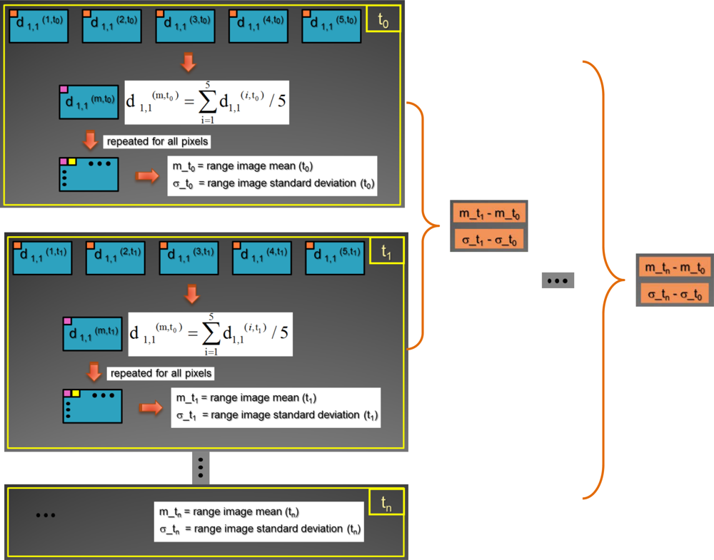
In all cases, the f = 5 frames (range images) acquired at each time (t_i) were averaged pixel by pixel in order to reduce the measurement noise; therefore the following term was estimated for each considered pixel:

$$d_{r,c}{}^{(m,t_i)}=\frac{\sum _{f=1}^5{d_{r,c}}^{(f,t_i)}}{f}$$

(1)

The term d_r,c^(f,ti) represents the measured distance by pixel in row r column c for the f-th acquired frame at the time t_i. Since the camera was fixed in each test, variations during the operation time of the mean (m_t_i) and standard deviation (σ_t_i) of the averaged range images were calculated. Since the tests were performed at different distances (and integration times), the relative variations of the mean (m_t_i) and standard deviation (σ_t_i), with respect to their initial values (m_t₀ and σ_t₀), were considered for each test in order to compare them:

$$m\_t_i=\frac{\sum _{r=r_{\text{min}}}^{r_{\text{max}}}\sum _{c=c_{\text{min}}}^{c_{\text{max}}}{d_{r,c}}^{(m,t_i)}}{n}$$

(2)

$$\sigma \_t_i=\sqrt{\frac{\sum _{r=r_{\text{min}}}^{r_{\text{max}}}\sum _{c=c_{\text{min}}}^{c_{\text{max}}}{(d_{r,c}{}^{(m,t_i)}-m\_t_i)}^2}{n-1}}$$

(3)

$$n=(r_{\text{max}}-r_{\text{min}}+1)*(c_{\text{max}}-c_{\text{min}}+1)$$

(4)

where r_min, r_max and c_min, c_max represent the row gap and the column gap of the sensor pixel considered in the analysis and n the number of considered pixels.

Figure 4 is a schematic representation of the data processing workflow, were the blue area represents the group of pixels considered for the analysis (this area is defined by r_min, r_max and c_min, c_max).

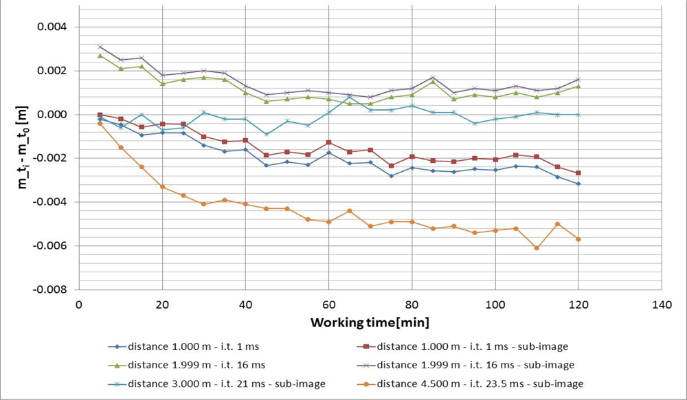
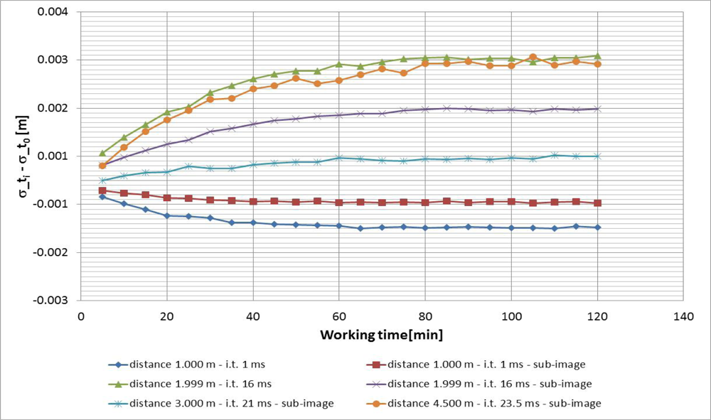
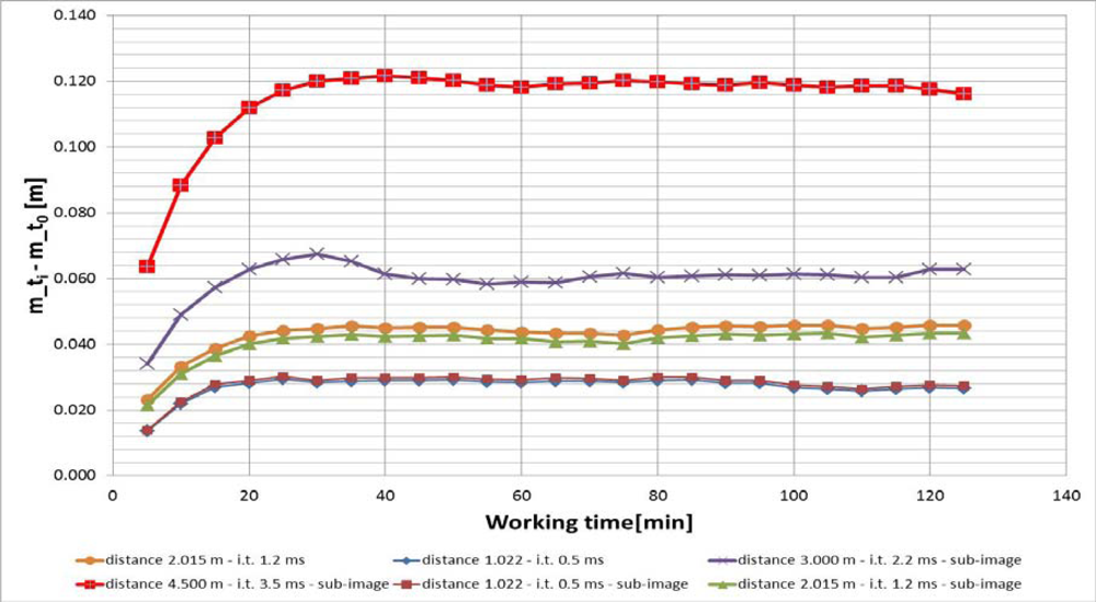
The variations of m_t_i and σ_t_i during two hours of camera acquisition are shown in Figures 5 and 6 respectively. In all cases a central sub-image of 84 × 96 pixels was considered, while in two cases (when the wall filled the entire range image) the entire image of 176 × 144 pixels was considered.

As can be observed from Figures 5 and 6, both the mean value and the standard deviation of the distance measurements vary during operation: a maximum variation of about −6 mm was detected for the mean value, while a maximum variation of about 3 mm was measured for the standard deviation. Since the calculated variations are nearly constant after 40 min of camera operation, a warm up period of 40 min is sufficient to achieve a good measurement stability for the SR-4000 camera. For this reason, all the following tests were performed after this warm-up period.

3.2. Test of the CamCube3.0 Camera

The procedure for testing the CamCube3.0 camera is identical to the one adopted for the SR-4000 camera. As in the previous case, after turning on the camera, five consecutive frames were acquired every five minutes for two hours of camera operation. The test was carried out at several distances (and integration times) between the front of the camera and the wall, in order to get more reliable results.

Since in this case no estimation of an “auto acquisition time” was available, the integration time was adjusted manually to limit pixel saturation and distance measurement noise.

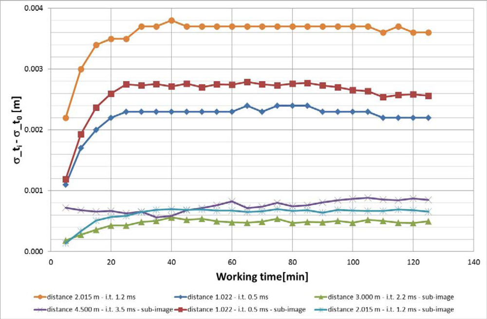
The variations of m_t_i and σ_t_i during two hours of camera acquisition are reported in Figures 7 and 8 respectively. In all cases a central sub-image of 106 × 150 pixels was considered, while in two cases (when the wall filled the entire range image), the entire image of 200 × 200 pixels was also considered.

As can be observed from Figures 7 and 8, both the mean value and the standard deviation of the distance measurements vary during operation: a maximum variation of about 120 mm was detected for the mean value, while a maximum variation of about 4 mm was measured for the standard deviation. As in the previous case, since the estimated variations are nearly constant after 40 min of camera operation, a warm up period of 40 min is sufficient to achieve a good measurement stability of the CamCube3.0 camera. The camera warm up period is highly recommended in this case, in order to avoid distance errors of several centimeters. Therefore, all the following tests were performed after this warm-up period.

4. Integration Time and Distance Measurement Precision

In the following, an estimation of the distance measurement precision of both the SR-4000 and the CamCube3.0 cameras is performed for varying image integration times.

4.1. Test on the SR-4000 Camera

In order to estimate the precision (standard deviation) of the distance measurements performed by the sensor pixels (n pixels), the following test was performed. The SR-4000 camera was positioned on a photographic tripod, parallel to a white wall. Then, 100 frames were acquired for several integration times reported in

Table 2. Results for three different positions of the SR-4000 camera, where i.t. is the integration time, m_σ is the mean value of the estimated standard deviations for all the pixels, m_Dm and std_Dm are the mean and standard deviation values of the range image respectively, m_Am is the mean value of the amplitude image and m_Cm is the mean value of the confidence map.

distance [m] =	1.00
n° frames [-] =	100

Table 2. Results for three different positions of the SR-4000 camera, where i.t. is the integration time, m_σ is the mean value of the estimated standard deviations for all the pixels, m_Dm and std_Dm are the mean and standard deviation values of the range image respectively, m_Am is the mean value of the amplitude image and m_Cm is the mean value of the confidence map.

i.t. [ms]	Mσ [m]	N° saturated pixels [-]	mDm [m]	StdDm [m]	mAm [-]	mCm [-]
3.500	0.0033	0	1.013	0.016	4,558	7.991
4.750	0.0030	0	1.014	0.016	5,240	7.996
6.000 (auto)	0.0028	96	1.013	0.017	5,895	7.998
7.250	0.0027	28	1.013	0.037	6,606	7.996
8.500	0.0043	334	1.000	0.114	7,784	7.894
9.750	0.0086	1,727	0.945	0.251	10,913	7.455

Table 2. Results for three different positions of the SR-4000 camera, where i.t. is the integration time, m_σ is the mean value of the estimated standard deviations for all the pixels, m_Dm and std_Dm are the mean and standard deviation values of the range image respectively, m_Am is the mean value of the amplitude image and m_Cm is the mean value of the confidence map.

distance [m] =	1.30
n° frames [-] =	100

Table 2. Results for three different positions of the SR-4000 camera, where i.t. is the integration time, m_σ is the mean value of the estimated standard deviations for all the pixels, m_Dm and std_Dm are the mean and standard deviation values of the range image respectively, m_Am is the mean value of the amplitude image and m_Cm is the mean value of the confidence map.

i.t. [ms]	mσ [m]	N° saturated pixels [-]	mDm [m]	StdDm [m]	mAm [-]	mCm [-]
8.500	0.0040	0	1.312	0.008	8,091	7.992
9.750	0.0037	0	1.311	0.009	8,833	7.995
11.000 (auto)	0.0035	0	1.311	0.009	9,558	7.997
12.250	0.0034	7	1.311	0.023	10,293	7.996
13.500	0.0037	60	1.309	0.062	11,097	7.980

Table 2. Results for three different positions of the SR-4000 camera, where i.t. is the integration time, m_σ is the mean value of the estimated standard deviations for all the pixels, m_Dm and std_Dm are the mean and standard deviation values of the range image respectively, m_Am is the mean value of the amplitude image and m_Cm is the mean value of the confidence map.

distance [m] =	1.60
n° frames [-] =	100

Table 2. Results for three different positions of the SR-4000 camera, where i.t. is the integration time, m_σ is the mean value of the estimated standard deviations for all the pixels, m_Dm and std_Dm are the mean and standard deviation values of the range image respectively, m_Am is the mean value of the amplitude image and m_Cm is the mean value of the confidence map.

i.t. [ms]	Mσ [m]	N° saturated pixels [-]	mDm [m]	StdDm [m]	mAm [-]	mCm [-]
16.750	0.0032	0	1.611	0.008	12,932	7.994
18.000	0.0030	0	1.611	0.008	13,630	7.996
19.250 (auto)	0.0029	0	1.610	0.008	14,319	7.997
20.500	0.0028	0	1.610	0.008	15,006	7.998
21.750	0.0028	2	1.610	0.016	15,679	7.998
23.000	0.0027	6	1.609	0.025	16,325	7.997

, were “auto” means the auto acquisition time suggested by the SR_3D_View software.

For each pixel i (each pixel is now individuated with only one letter (instead of row r and column c) to improve clarity of presentation), the mean value (d_i,m) and the standard deviation (σ_i) of the acquired distance measurements (number of frames f = 100) were estimated:

$$d_{i,m}=\frac{\sum _{t=1}^f{d}_{i,t}}{f}$$

(5)

$${\sigma }_i=\sqrt{\frac{\sum _{t=1}^f{(d_{i,t}-d_{i,m})}^2}{n-1}}$$

(6)

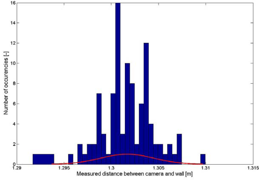
In Figure 9 a histogram of the 100 distance measurements performed by the central pixel with an integration time of 11 ms for an approximate distance of 1.30 m between camera and wall is reported. The term “approximate distance” is used since the distance between the camera and its orthogonal projection on the wall was measured with a metal tape and the exact shape of the wall was unknown. However, this doesn’t affect the results of the test as only relative variations of the distance measurements are considered in the following. Suitable accuracy tests have already been performed during other experiments [23] for the SR-4000 camera and will be performed for the CamCube3.0 too in the future.

Figure 9 shows that the maximum of the distance measurement distribution is very close to the approximated distance value between camera and wall.

In order to compare data acquired with different integration times, the following were estimated: the mean value of the estimated standard deviations (m_σ) for all the pixels, which represents the mean precision of the sensor; the mean value of the range image (averaged over 100 frames) (m_Dm) and its standard deviation (std_Dm); the mean value of the amplitude image (averaged over 100 frames) (m_Am) and the mean value of the confidence map (averaged over 100 frames) (m_Am).

$$m_{\sigma }=\frac{\sum _{i=1}^n{\sigma }_i}{n}$$

(7)

$$m_{Dm}=\frac{\sum _{i=1}^n{d}_{i,m}}{n}$$

(8)

$$\mathit{st}{d}_{Dm}=\sqrt{\frac{\sum _{i=1}^n{\left(d_{i,m}-m_{Dm}\right)}^2}{n-1}}$$

(9)

$$m_{Am}=\frac{\sum _{i=1}^n\sum _{t=1}^f{A}_{i,t}}{n\cdot f}$$

(10)

$$m_{Cm}=\frac{\sum _{i=1}^n\sum _{t=1}^f{C}_{i,t}}{n\cdot f}$$

(11)

where A_i,t and C_i,t are the amplitude and the confidence values for the i-th pixel at the t-th frame respectively. This procedure was repeated three times, positioning the camera at different distances from the wall. The results are reported in Table 2.

As can be seen from Table 2, for each camera position, with data acquired with the auto acquisition time we have: the lowest mean value of the pixel standard deviations (m_σ), so more precise distance measurements; a null or negligible number of saturated pixels, which is a fundamental condition in order to avoid gross errors from the acquired data; a less noisy distribution of the distance measurements over the acquired area of the wall, which is represented by small values of the std_Dm term; the maximum value of the m_Cm term, which represents the mean quality of the measurements performed by the pixels. Since the real distance between the camera and the wall was measured with a metal tape (without considering the real shape of the wall), no evaluation of absolute measurement accuracy can be done in this case; nevertheless, the variations of the mean value of the measured distances (m_Dm) considering different integration times are very small, limited to some millimeters when only few saturated pixels appear. For these reasons, the auto acquisition time will be adopted during data acquisition with the SR-4000 camera instead of adjusting it manually.

In Figure 10 a 3D representation of the σ_i term for each pixel over the whole sensor along with the amplitude image (averaged over 100 frames) are reported.

Figure 10(a) shows that the measurement precision is better for the central pixels than the pixels at the corners of the sensor. In the case (1.30 m, i.t. = 11 ms), values of the pixel precision up to 0.013 m are observed at the image corners. This is directly related to the amplitude of the reflected signal: since the amplitude is lower at the corners of the image (yellow and green areas in Figure 10(b)), distance measurements with higher standard deviation and therefore less precision are present. In the figure, a few saturated pixels in the central part of the image are present, which gives a few higher values in the 3D representation (Figure 10(a)). This test shows the important relation between the strength of the reflected signal and the distance measurement precision. For this reason, it is important to properly adjust the integration time in order to have the highest amplitude values without reaching pixel saturation. The results show that the auto acquisition time suggested by the SR_3D_View software completely adheres to this observation.

4.2. Test of the CamCube3.0 Camera

The same test described in the previous section was performed using the CamCube3.0 camera. Since the software delivered with this camera does not automatically adjust the integration time, this parameter was adjusted manually. Several integration times were adopted spanning a small range of all possible integration times (from 20 to 50,000 μs for this camera), in order to have low noise of the distance measurements and a small number of saturated pixels. With the SR-4000 camera a confidence map is delivered, however the CamCube3.0 delivers a flag matrix with the acquired data. The flag matrix indicates for each pixel if the camera detected problems with the measurement process. In particular, the meaning of the flags is reported in

Table 3. Possible values in the flag matrix delivered by the CamCube3.0 camera.

Flag Meaning	Value [-]
Invalid measurement	1
Saturation	2
SBI (Suppression of Background Illumination)	4
Low signal	8
Inconsistent	10

[24].

Obviously the zero value means that no problems occurred during the measurement. Therefore, the expected quality of the acquired data could be obtained by computing the mean value of the flag matrix for the considered frame: higher the mean value, more problems occurred during the acquisition phase. For this reason, the mean value of the flag matrix (averaged over 100 frames) (m_Fm) was estimated for a given pixel as:

$$m_{Fm}=\frac{\sum _{i=1}^n\sum _{t=1}^f{F}_{i,t}}{n\cdot f}$$

(12)

where F_i,t is the flag value for the i-th pixel at the t-th frame. Since the i.t. was adjusted manually, several integration times were employed for each of the three cases (

Table 4. Results for three different positions of the CamCube3.0 camera, where i.t. is the integration time, m_σ is the mean value of the estimated standard deviations for all the pixels, m_Dm and Std_Dm are the mean and standard deviation values of the range image respectively, m_Am is the mean value of the amplitude image and m_Fm is the mean value of the flag matrix.

distance [m] =	1.00
n° frames [-] =	100

Table 4. Results for three different positions of the CamCube3.0 camera, where i.t. is the integration time, m_σ is the mean value of the estimated standard deviations for all the pixels, m_Dm and Std_Dm are the mean and standard deviation values of the range image respectively, m_Am is the mean value of the amplitude image and m_Fm is the mean value of the flag matrix.

i.t. [ms]	Mσ [m]	N° saturated pixels [-]	mDm [m]	StdDm [m]	mAm [-]	mFm [-]
0.050	0.0222	0	0.977	0.008	810	0.0000
0.100	0.0128	0	0.986	0.006	1,849	0.0000
0.150	0.0096	5	0.996	0.005	2,968	0.0000
0.200	0.0080	7	1.003	0.004	4,170	0.0001
0.250	0.0070	6	1.007	0.004	5,460	0.0000
0.300	0.0063	1	1.011	0.004	6,799	0.0000
0.350	0.0058	1	1.014	0.005	8,141	0.0000
0.400	0.0054	1	1.018	0.005	9,449	0.0000
0.450	0.0051	23	1.020	0.005	10,722	0.0013
0.500	0.0049	488	1.023	0.005	11,949	0.0317
0.550	0.0047	2,100	1.025	0.005	13,129	0.1416

Table 4. Results for three different positions of the CamCube3.0 camera, where i.t. is the integration time, m_σ is the mean value of the estimated standard deviations for all the pixels, m_Dm and Std_Dm are the mean and standard deviation values of the range image respectively, m_Am is the mean value of the amplitude image and m_Fm is the mean value of the flag matrix.

distance [m] =	1.30
n° frames [-] =	100

Table 4. Results for three different positions of the CamCube3.0 camera, where i.t. is the integration time, m_σ is the mean value of the estimated standard deviations for all the pixels, m_Dm and Std_Dm are the mean and standard deviation values of the range image respectively, m_Am is the mean value of the amplitude image and m_Fm is the mean value of the flag matrix.

i.t. [ms]	mσ [m]	N° saturated pixels [-]	mDm [m]	StdDm [m]	mAm [-]	mFm [-]
0.100	0.0189	0	1.290	0.010	1,036	0.000
0.150	0.0137	0	1.295	0.008	1,670	0.000
0.200	0.0112	4	1.301	0.007	2,332	0.000
0.250	0.0096	1	1.307	0.006	3,020	0.000
0.300	0.0085	3	1.311	0.006	3,740	0.000
0.350	0.0077	5	1.315	0.006	4,495	0.000
0.400	0.0072	3	1.318	0.006	5,279	0.000
0.450	0.0067	1	1.321	0.006	6,081	0.000
0.500	0.0063	1	1.323	0.007	6,889	0.000
0.550	0.0060	0	1.326	0.007	7,691	0.000
0.600	0.0057	0	1.328	0.007	8,485	0.000
0.650	0.0054	0	1.330	0.007	9,265	0.000
0.700	0.0053	8	1.332	0.007	10,030	0.000
0.750	0.0051	78	1.335	0.007	10,778	0.005
0.800	0.0050	368	1.338	0.008	11,509	0.023
0.850	0.0048	1,017	1.341	0.009	12,223	0.068

Table 4. Results for three different positions of the CamCube3.0 camera, where i.t. is the integration time, m_σ is the mean value of the estimated standard deviations for all the pixels, m_Dm and Std_Dm are the mean and standard deviation values of the range image respectively, m_Am is the mean value of the amplitude image and m_Fm is the mean value of the flag matrix.

distance [m] =	1.60
n° frames [-] =	100

Table 4. Results for three different positions of the CamCube3.0 camera, where i.t. is the integration time, m_σ is the mean value of the estimated standard deviations for all the pixels, m_Dm and Std_Dm are the mean and standard deviation values of the range image respectively, m_Am is the mean value of the amplitude image and m_Fm is the mean value of the flag matrix.

i.t. [ms]	mσ [m]	N° saturated pixels [-]	mDm [m]	StdDm [m]	mAm [-]	mFm [-]
0.250	0.0117	0	1.603	0.009	1,889	0.000
0.300	0.0103	1	1.608	0.008	2,331	0.000
0.350	0.0093	1	1.612	0.008	2,784	0.000
0.400	0.0085	2	1.615	0.008	3,249	0.000
0.450	0.0079	1	1.617	0.008	3,732	0.000
0.500	0.0074	2	1.620	0.008	4,230	0.000
0.550	0.0070	18	1.622	0.008	4,742	0.000
0.600	0.0066	37	1.624	0.009	5,263	0.000
0.650	0.0063	53	1.627	0.009	5,789	0.000
0.700	0.0060	46	1.628	0.009	6,319	0.000
0.750	0.0058	45	1.631	0.009	6,845	0.000
0.800	0.0056	31	1.632	0.009	7,369	0.000
0.850	0.0054	25	1.634	0.009	7,889	0.000
0.900	0.0053	13	1.636	0.009	8,402	0.000
0.950	0.0051	9	1.638	0.009	8,908	0.000
1.000	0.0050	3	1.641	0.009	9,408	0.000
1.050	0.0049	3	1.643	0.009	9,901	0.000
1.100	0.0048	23	1.646	0.009	10,385	0.001
1.150	0.0047	67	1.649	0.009	10,864	0.004
1.200	0.0046	176	1.652	0.009	11,330	0.012
1.250	0.0045	383	1.655	0.009	11,793	0.026
1.300	0.0045	694	1.658	0.009	12,243	0.047
1.350	0.0044	1,090	1.661	0.009	12,692	0.075

).

As can be seen from Table 4, the m_σ term decreases when i.t. increases, as was expected. The number of pixels having a flag different from zero varies with increasing integration time in a non-linear way. The mean precision (m_σ) is about 0.002 m better for the SR-4000 camera compared to the CamCube3.0 camera in the three tests (same adopted procedure for both cameras).

The variations of the mean value of the measured distances (m_Dm) for the Camcube3.0considering different integration times are bigger than SR-4000 camera even if smaller gaps of i.t. are considered for the CamCube3.0 camera: in this case, variations up to 0.040–0.050 m are observed, even with a small number of saturated pixels. A similar behavior of non-negligible distance variations with changing integration time was also detected for other previous PMD camera models. For example, in [25] distance variations of several centimeters were observed for the PMD19k camera.

In Figure 11, a 3D representation of the σ_i term of each pixel for the whole sensor and the amplitude image (averaged over 100 frames) are reported. Figure 11 shows that the measurement precision is better for the central pixels with respect to pixels at the corners of the sensor since the amplitude of the reflected signal is higher in the center. In the displayed case (i.t. = 0.7 ms, 1.30 m of distance), values of the pixel precision up to 0.010 m are observed at the image corners. As mentioned before, this variation is directly related to the amplitude of the reflected signal: since the amplitude is lower at the corners of the image (blue areas in Figure 11(b)), distance measurements with higher standard deviation and therefore less precision are present. Comparing Figure 10(a) with Figure 11(a), one can see that the sensor precision is more homogeneous for adjacent pixels in the SR-4000. Again, this is a direct consequence of the amplitude distribution over the sensor: for the CamCube3.0 camera the central amplitudes are quadruple that of the corners, while for the SR-4000 camera the central amplitudes are double that of the corners.

This test shows the relation between integration time, distance measurement precision and distance measurement values for the CamCube3.0 camera. It is necessary to properly adjust the integration time, taking into account the distance variations which exist even with small changes of the i.t. parameter. Future work will be performed to take into account this effect in a proper distance calibration model.

6. Conclusions and Future Work

In this paper experimental comparisons between the SR-4000 and CamCube3.0 cameras have been reported in order to evaluate their performance and to give some procedures for testing data from ToF cameras.

After a brief overview of commercial ToF cameras available on the market and the main specifications of the tested devices, two topics have been presented. First, the influence of camera warm up on distance measurements was analyzed: a warm up of 40 min is suggested to obtain distance measurement stability, especially in the case of the CamCube3.0 camera, for which warm-up distance measurement variations up to 0.12 m have been found. Secondly, the distance measurement precision variation of the cameras with varying integration time was examined. Distance measurement precisions of 3–4 mm have been obtained in both cases, with improvements in the measurement precision increasing integration time (and consequently the amplitude of the reflected signal), as it was expected. Nevertheless, with changing the integration time of the CamCube3.0 camera, distance variations up to 0.040–0.050 m are observed, while for the SR-4000 camera variations are very small, limited to 0.004–0.005 m when only few saturated pixels appear. This test shows the important relation between integration time, distance measurement precision and distance measurement values for the CamCube3.0 camera. It is necessary to properly adjust the integration time, taking into account the distance variations which exist also with small changes of the integration time.

During the tests, a qualitative evaluation of sunlight influence on distance measurements has been performed too, in order to test the sensor sensibility to sunlight rays. Since almost all ToF cameras based on the phase shift measurement use an infrared signal to measure distances, one main aspect to be considered is the influence of sunlight on the acquired data. Many recent ToF cameras support the Suppression of Background Illumination (SBI) modality or an equivalent IR-suppression scheme, allowing the usage of the devices also in outdoor applications. Nevertheless, data acquisition with ToF cameras using near-infrared wavelength in direct sunlight could still be a hard task. Previous works, i.e., [22,26,27], have already reported about problems of noisy data in outdoor acquisitions. Some first tests performed by our research group show that the CamCube3.0 camera is more robust to sunlight than the SR-4000 camera thanks to its SBI system, as it was expected from the information reported in the manufacturer data sheets of the two devices. In fact, the SR-4000 has been designed for indoor use and it has not to be used in direct sunlight [28], while the CamCube3.0 camera is equipped with the PhotonICs^®PMD 41k-S2 sensor [24]. It includes the Suppression of Background Illumination (SBI), which is suitable for both indoor and outdoor environments. Nevertheless, specific tests will be performed in the future in order to verity if the acquired data are degraded by sunlight even with SBI.

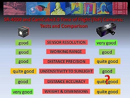
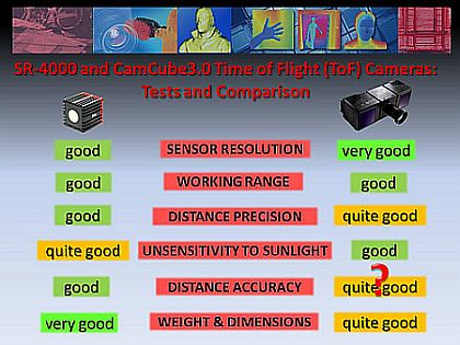
Figure 13 summarizes the results of the tests. These were confirmed by the camera manufacturer agents during the International Workshop on Range-imaging Sensors and Applications 2011 [29].

The red question mark reported for the distance measurement accuracy of the CamCube3.0 in Figure 13 is due to the fact that the distance measurement accuracy of the CamCube3.0 camera is not exactly known, but some preliminary tests performed by our group and already published works [16] on the previous camera model (CamCube2.0) shown a distance measurement accuracy of some centimeters. Future works will estimate the actual distance measurement accuracy of the CamCube3.0 camera.

References

- Albota, M.A.; Heinrichs, R.M.; Kocher, D.G.; Fouche, D.G.; Player, B.E.; Obrien, M.E.; Aull, G.F.; Zayhowski, J.J.; Mooney, J.; Willard, B.C.; Carlson, R.R. Three-dimensional imaging laser radar with a photon-counting avalanche photodiode array and microchip laser. Appl. Opt 2002, 41, 7671–7678. [Google Scholar]
- Rochas, A.; Gösch, M.; Serov, A.; Besse, P.A.; Popovic, R.S. First fully integrated 2-D array of single-photon detectors in standard CMOS technology. IEEE Photon. Technol. Lett 2003, 15, 963–965. [Google Scholar]
- Gvili, R.; Kaplan, A.; Ofek, E.; Yahav, G. Depth keying. Proc. SPIE 2003, 5249, 534–545. [Google Scholar]
- Lange, R. Time-of-Flight range imaging with a custom solid-state image sensor. Proc. SPIE 1999, 3823, 180–191. [Google Scholar]
- Anderson, D.; Herman, H.; Kelly, A. Experimental Characterization of Commercial Flash Ladar Devices. Proceedings of International Conference on Sensing Technologies, Palmerston North, New Zealand, 21–23 November 2005.
- Kahlmann, T.; Remondino, F.; Ingensand, H. Calibration for increased accuracy of the range imaging camera SwissRanger. Int. Arch. Photogrammetry, Remote Sensing and Spatial Information Sciences 2006, XXXVI, 136–141. [Google Scholar]
- Beder, C.; Koch, R. Calibration of Focal Length and 3D Pose Based on the Reflectance and Depth Image of a Planar Object. Proceedings of the Dynamic 3D Imaging Workshop, Heidelberg, Germany, 11 September 2007; pp. 11–20.
- Lindner, M.; Kolb, A. Calibration of the intensity related distance error of the PMD ToF-camera. Proc. SPIE 2007, 6764, 67640W. [Google Scholar]
- Karel, W.; Dorninger, P.; Pfeifer, N. Situ Determination of Range Camera Quality Parameters by Segmentation. Proceedings of VIII International Conference on Optical 3-D Measurement Techniques, Zurich, Switzerland, 9–12 July 2007; pp. 109–116.
- Fuchs, S.; Hirzinger, G. Extrinsic and Depth Calibration of ToF-Cameras. Proceedings of IEEE Conference on Computer Vision and Pattern Recognition, Anchorage, AK, USA, 23–28 June 2008; pp. 1–6.
- Kim, Y.M.; Chan, D.; Theobalt, C.; Thrun, S. Design and Calibration of a Multi-View ToF Sensor Fusion System. Proceedings of IEEE CVPR Workshop on Time-of-Flight Computer Vision, Anchorage, AK, USA, 23–28 June 2008; pp. 1–7.
- Lichti, D. Self-calibration of a 3D range camera. Int. Arch. Photogramm. Remote Sens. Spatial Inf. Sci 2008, XXXVII, 927–932. [Google Scholar]
- Schiller, I.; Beder, C.; Koch, K. Calibration of a PMD-camera using a planar calibration pattern together with a multi-camera setup. Int. Arch. Photogramm. Remote Sens. Spatial Inf. Sci 2008, XXXVII, 297–302. [Google Scholar]
- Rapp, H.; Frank, M.; Hamprecht, F.A.; Jähne, B. A theoretical and experimental investigation of the systematic errors and statistical uncertainties of Time-of-Flight-cameras. IJISTA 2008, 5, 402–413. [Google Scholar]
- Westfeld, P.; Mulsow, C.; Schulze, M. Photogrammetric Calibration of Range Imaging Sensors Using Intensity and Range Information Simultaneously. Proceedings of 9th Conference on Optical 3-D Measurement Techniques, Vienna, Austria, 1–3 July 2009.
- Boehm, J.; Pattinson, T. Accuracy of exterior orientation for a range camera. Int. Arch. Photogramm. Remote Sens. Spatial Inf. Sci 2010, XXXVIII, 103–108. [Google Scholar]
- Chiabrando, F.; Piatti, D.; Rinaudo, F. SR-4000 ToF camera: further experimental tests and first applications to metric surveys. Int. Arch. Photogramm. Remote Sens. Spatial Inf. Sci 2010, XXXVIII, 149–154. [Google Scholar]
- Lichti, D.; Kim, C.; Jamtsho, S. An integrated bundle adjustment approach to range camera geometric self-calibration. ISPRS J. Photogramm 2010, 65, 360–368. [Google Scholar]
- SoftKinetic. Available online: http://www.softkinetic.com/ (accessed 20 December 2011).
- Weyer, C.A.; Bae, K.; Lim, K.; Lichti, D. Extensive metric performance evaluation of a 3D range camera. Int. Arch. Photogramm. Remote Sens. Spatial Inf. Sci 2008, XXXVII, 939–944. [Google Scholar]
- Steiger, O.; Felder, J.; Weiss, S. Calibration of Time-of-Flight Range Imaging Cameras. Proceedings of the 15th IEEE ICIP, San Diego, CA, USA, 12–15 October 2008; pp. 1968–1971.
- Ollikkala Arttu, V.H.; Mäkynen, A.J. Range Imaging Using a Time-of-Flight 3D Camera and a Cooperative Object. Proceedings of IEEE Conference on Instrumentation and Measurement Technology, Singapore, 5–7 May 2009; pp. 817–821.
- Chiabrando, F.; Chiabrando, R.; Piatti, D.; Rinaudo, F. Sensors for 3D imaging: Metric Evaluation and calibration of a CCD/CMOS Time-of-Flight camera. Sensors 2009, 9, 10080–10096. [Google Scholar]
- PMD Technologies GmbH. Available online: http://www.pmdtec.com/ (accessed 10 July 2011).
- Radmer, J.; Fuste, P.; Schmidt, H.; Krüger, J. Incident Light Related Distance Error Study and Calibration of the PMD-Range Imaging Camera. Proceedings of IEEE Computer Society Conference on Computer Vision and Pattern Recognition Workshops, Anchorage, AK, USA, 23–28 June 2008; pp. 1–6.
- Klose, R.; Penlington, J.; Ruckelshausen, A. Usability study of 3D time-of-flight cameras for automatic plant phenotyping. Applied Sciences 2009, 69, 93–105. [Google Scholar]
- Kraft, M.; Salomão de Freitas, N.R.; Munack, A. Test of a 3D Time of Flight Camera for Shape Measurements of Plants. Proceedings of CIGR Workshop on Image Analysis in Agriculture, Budapest, Hungary, 26–27 August 2010; pp. 108–116.
- Mesa Imaging. Available online: http://www.mesa-imaging.ch/ (accessed 10 July 2011).
- International Workshop on Range-imaging Sensors and Applications. 2011. Available online: http://risa2011.fbk.eu/home (accessed 10 July 2011).
Figure 1.
SR-4000 (left) and CamCube3.0 (right) tested in this work.
Figure 2.
Visualization of data acquired with the SR-4000 camera: amplitude image (arbitrary units) and range image (m) (up, from left to right); confidence map (units from 0 to 8) and 3D point cloud already corrected by lens distortion (manufacturer calibration) (bottom, from left to right).
Figure 3.
Visualization of data acquired with the CamCube3.0 camera: Amplitude image (arbitrary units) and intensity image (arbitrary units) (up, from left to right); range image (m), flag matrix (units from 0 to 10) and 3D point cloud without lens distortion correction (bottom, from left to right).
Figure 4.
Schematic representation of the data processing workflow for each warm up test (f = 5).
Figure 5.
Relative variations of the mean value of averaged range images during the warm-up time of several tests for the SR-4000 (i.t. = integration time).
Figure 6.
Relative variations of the standard deviation for averaged range images during the warm-up time of several tests for the SR-4000 (i.t. = integration time).
Figure 7.
Relative variations of the mean value for averaged range images during the operation time of several tests for the CamCube3.0 (i.t. = integration time).
Figure 8.
Relative variations of the standard deviation for averaged range images during the working time of several tests for the CamCube3.0 (i.t. = integration time).
Figure 9.
Histogram of the 100 distance measurements performed by the central pixel of the SR-4000 camera with an integration time of 11 ms (approximate distance camera-wall: 1.30 m).
Figure 10.
SR-4000 (a) 3D representation of the σi over the whole sensor (the color-bar is in meters) and (b) amplitude image (the color-bar is in arbitrary units) for data acquired with the auto acquisition time (distance camera-wall: 1.30 m; i.t. = 11 ms).
Figure 11.
CamCube3.0 (a) 3D representation of the σi over the whole sensor (the color-bar is in meters) and (b) amplitude image (the color-bar is in arbitrary units) (distance camera-wall: 1.30 m; i.t. = 7 ms).
Figure 13.
Comparison between SR-4000 camera (left) and CamCube3.0 camera (right) based on the performed tests.