A Novel Satellite Mission Concept for Upper Air Water Vapour, Aerosol and Cloud Observations Using Integrated Path Differential Absorption LiDAR Limb Sounding

Abstract

We propose a new satellite mission to deliver high quality measurements of upper air water vapour. The concept centres around a LiDAR in limb sounding by occultation geometry, designed to operate as a very long path system for differential absorption measurements. We present a preliminary performance analysis with a system sized to send 75 mJ pulses at 25 Hz at four wavelengths close to 935 nm, to up to 5 microsatellites in a counter-rotating orbit, carrying retroreflectors characterized by a reflected beam divergence of roughly twice the emitted laser beam divergence of 15 μrad. This provides water vapour profiles with a vertical sampling of 110 m; preliminary calculations suggest that the system could detect concentrations of less than 5 ppm. A secondary payload of a fairly conventional medium resolution multispectral radiometer allows wide-swath cloud and aerosol imaging. The total weight and power of the system are estimated at 3 tons and 2,700 W respectively. This novel concept presents significant challenges, including the performance of the lasers in space, the tracking between the main spacecraft and the retroreflectors, the refractive effects of turbulence, and the design of the telescopes to achieve a high signal-to-noise ratio for the high precision measurements. The mission concept was conceived at the Alpbach Summer School 2010.

1. Introduction

The topic for the Alpbach Summer School 2010 in Austria was “New Space Missions for Understanding Climate Change”. Early career scientists and engineers from many countries formed working groups to devise new space missions to tackle this challenging subject. Following the summer school, one mission concept was chosen for further development at a subsequent workshop in Obergurgl, the outcome of which is described in this paper. At the core of the mission chosen for further study was a novel active limb-sounding instrument, used as part of a multi-instrument measurement approach to observing three key climate change variables: water vapour, clouds and aerosols.

Water vapour in the upper troposphere-lower stratosphere (UTLS) region has an important role in determining the atmospheric temperature profile and tropopause structure [1,2]. Observations are particularly challenging because of the low concentrations, and the poor vertical resolution of conventional passive nadir instruments in this region. However, this information is vital in general circulation models (GCMs) for the understanding and future prediction of the Earth’s climate system. Aerosols and clouds, and their interactions, have also been identified as key climate change uncertainties, and observations of these in the UTLS are also limited [3].

Currently, several ground-based systems use differential optical absorption spectroscopy (DOAS) to detect low concentrations of trace gases by comparing path-integrated measurements over a continuous range of wavelengths. We propose an analogous spaceborne system, looking through the limb of the atmosphere at a few discrete wavelengths to detect differential absorption due to water vapour. By combining such a limb-looking LiDAR with a nadir-looking range-resolved LiDAR, this mission would provide water vapour and aerosol measurements in the UTLS and above of unprecedented accuracy and resolution. The addition of an imaging spectrometer operating in the visible and infrared range allows cloud microphysical properties to be retrieved in the same location, enabling process studies of cloud-aerosol-climate interactions and the reduction of key uncertainties in climate prediction.

A nadir water vapour LiDAR was proposed to ESA in 2002 as the WALES candidate Earth Explorer mission [4]. The instrument concept presented in this paper builds on the laser and nadir LiDAR system development begun for the WALES mission.

Section 2 presents the scientific motivation and requirements for the new mission. Section 3 gives an overview of the mission concept, while Section 4 presents the preliminary performance calculations for the system. Section 5 presents the technical implementation in more detail and Section 6 outlines the main technical challenges associated with the concept.

2. Motivation and Background

2.1. The Importance of Upper Air Water Vapour, Clouds and Aerosols

Water vapour is the most important greenhouse gas, contributing about 50% towards the Earth’s greenhouse effect, followed by clouds which contribute around 25% [5]. The radiative balance of the atmosphere is particularly sensitive to changes in the UTLS, as this is where most of the Earth’s thermal radiation escapes into space, and where cirrus clouds trap this outgoing radiation. For example, decreasing water vapour in the stratosphere has been identified as slowing the rate of increase of global surface temperature between 2000 and 2009 by about 25% [6], however it is not clear if the observed decadal variability in stratospheric water vapour is a driver or rather a response to climate change.

Water vapour in the stratosphere originates from transport through the tropopause region [7] and from the oxidation of methane, especially in the higher stratosphere. Transport is mainly induced by deep convection in the tropics passing the cold trap tropopause ([6] and references therein). Absolute amounts are low, less than 10 ppmv [8], but nevertheless are of crucial importance, both radiatively and for atmospheric chemistry, for example through an indirect destructive effect on the ozone layer as shown in [9]. Furthermore water vapour can be used as a tracer to study atmospheric dynamics such as stratosphere–troposphere exchange processes or the injection of trace gases into the stratosphere [10]. Important processes of this kind are for example the tropopause folds at midlatitudes or tropopause inversion layers [11], which are associated with strong peaks in the atmospheric stability above the tropopause. Their formation mechanisms are not well understood but the radiative effects of water vapour in combination with ozone may have a substantial impact [12].

The UTLS is also of interest because it is the region where aircraft fly, emitting carbon dioxide, water vapour, nitrous oxide and aerosols, forming contrails and having an impact on cirrus clouds and the radiative budget. Aerosol-cloud interactions are key here, and also poorly understood: the fourth report of the Intergovernmental Panel on Climate Change attributes the largest uncertainties and lowest scientific understanding of radiative forcing to aerosols and their direct and indirect albedo effects [13].

Aerosols in the UTLS affect the Earth’s radiation budget by reflecting and absorbing incoming radiation. The scattering of shortwave radiation leads to a cooling of the climate system, and the absorption of longwave radiation to an increased heating rate [14]. Aerosols also can affect the climate in an indirect way by modifying cloud properties, for example droplet size, quantity of cloud drops, cloud albedo, liquid water content and cloud lifetime. As a third effect, aerosols may have an influence on atmospheric chemistry through their indirect modification of the concentration of several gases, especially greenhouse gases [15]. The stratospheric concentrations of aerosol particles are in general quite small compared to tropospheric aerosol, apart from the high concentrations found after volcanic eruptions. The aerosol optical thickness in the stratosphere is typically an order of magnitude smaller than in the troposphere [16].

Cirrus clouds are ice clouds found in the upper troposphere, and cover about 30% of the globe on average over a year [17]. Cirrus clouds affect the Earth’s radiation balance by reducing the amount of shortwave radiation reaching the surface, and reducing the longwave radiation emitted back to space. The net effect on the surface radiation budget is dependent on the microphysical properties of the clouds such as ice water content, number density and size of ice crystals as well as thickness. Theoretical calculations suggest that optically thin cirrus (e.g., a contrail) generally has a warming effect whereas optically thick cirrus has a cooling effect. The net effect is still uncertain although it is generally believed that cirrus has a net warming effect [18].

Other high altitude clouds are also likely to have a net warming effect. A colder stratosphere in combination with a higher water vapour content will increase the probability of the formation of ice clouds in the lower stratosphere: polar stratospheric clouds. These clouds play a major role in the heterogeneous ozone chemistry and the decrease in ozone in polar winter, and require continued observation and better characterization for model validation [19,20]. Polar mesospheric clouds (noctilucent clouds) are thin layers of nanometer-sized ice particles that occur at even higher altitudes: between 82 and 87 km in the high-latitude summer mesosphere [21]. Their formation is very sensitive to the mesopheric environment, and changes in their frequency of occurrence, brightness and altitude could be related to climate change [22], so continued observation of these phenomena is necessary.

In contrast to the tropospheric water vapour increase, which is well simulated in global climate models, modelled past and projected future stratospheric water vapour variations significantly disagree between different GCMs [23,24]. Bias correction is also a challenge for the assimilation of observations of humidity [25]; accurate observations of stratospheric water vapour at high vertical resolution would allow more stringent testing of the models, and better exploitation of existing satellite and radiosonde data in data assimilation systems. All these uncertainties must be understood in order to make better observations and predictions of climate change.

2.2. Current Capabilities for Measuring Water Vapour, Clouds and Aerosols in the UTLS and above

The longest stratospheric measurement record comes from the radiosonde network. Sondes provide high resolution vertical profiles but are sparsely distributed across the globe, and both sonde type and reporting practices differ at different sites. Wang et al. [26] compared the performance of two types of operational radiosonde with a more accurate dew-point hygrometer and found that the radiosondes were insensitive to humidity changes in the upper troposphere, leading to potential errors in the climate record derived from these measurements. Sun et al. [27] also detect a dry bias which increases with altitude, and note the difficulty of collocating sonde profiles with other data sources, in part because of the drift of the balloon as it ascends.

Satellites are now also used to measure atmospheric humidity, providing much better spatial and temporal coverage than sondes. Infrared sounders such as SEVIRI on Meteosat Second Generation and the High-resolution Infrared Radiation Sounder (HIRS) provide information on upper-tropospheric humidity, but these nadir sounders have broad weighting functions that limit their vertical resolution. Deriving profile information from a top-of-atmosphere brightness temperature requires good a priori information on the atmospheric temperature structure, and the largest differences between different observations, models and reanalyses are seen in the upper troposphere and stratosphere [3].

Limb sounders have narrower weighting functions, with a pronounced peak at the altitude corresponding to the tangent point. This improves vertical resolution whilst still offering good coverage, at the expense of complex radiative transfer and difficult retrievals in the lower atmospheric layers due to increased scattering. Several satellites currently make passive limb measurements of water vapour, usually as part of missions measuring a wide range of atmospheric species. The Michelson Interferometer for Passive Atmospheric Sounding (MIPAS) on Enivsat, launched in 2002, is a mid-infrared Fourier transform spectrometer which can measure water vapour in the mesosphere, lower thermosphere, stratosphere and upper troposphere, at a vertical resolution of 3 km. The Odin satellite, launched in 2001 has a combined payload of the Sub-Millimeter Radiometer (SMR), and the Optical Spectrograph and Infrared Imaging Spectrum (OSIRIS), and also can be used to derive water vapour at 3 km vertical resolution, although 50% of its operational time is spent making astronomical rather than Earth observations. Higher vertical resolution is achieved by the Microwave Limb Sounder (MLS), launched in 2004 on Aura. It also observes thermal emission in the limb, and has a vertical resolution of 1.5 km at 200 hPa, reducing to 5 km in the mesosphere. The Tropospheric Emission Spectrometer (TES), also on Aura, has both nadir- and limb-viewing modes for water vapour. TES has a high spectral resolution but a relatively small swath (5.3 × 8.5 km) and nadir footprint (0.53 × 5.3 km). In limb mode, TES observes a region with a ground footprint of 26 km × 41.8 km, with a height resolution of 2.3 km and vertical coverage from 0 to 33 km.

Various occultation techniques are also used to measure water vapour. Water vapour profiles have recently been retrieved from SCIAMACHY (SCanning Imaging Absorption spectroMeter for Atmospheric CartograpHY) solar occultation data for an altitude range of 15–45 km with a vertical resolution of 2.6 km. However, the spectral resolution of SCIAMACHY is not high enough to resolve water vapour lines, which leads to additional correction steps in the retrieval algorithm [28]. The Atmospheric Chemistry Experiment, onboard the Canadian satellite SCISAT-1, carries a Fourier transform spectrometer for solar occultation profiles of water vapour. Vertical resolution is 3 to 4 km and the instrument has been making measurements since 2003. Nassar et al. [29] suggest that retrieved water vapour profiles have low measurement error, and are subject to a random error of less than 2.0% for the stratosphere (with higher values in the troposphere and mesosphere). The Global Ozone Monitoring by Occultation of Stars (GOMOS) uses stellar occultation to retrieve vertical profiles of atmospheric constituents, with a vertical resolution of 2–4 km. The signal-to-noise ratio for water vapour is low, but the retrieval has recently been improved through refined calibration procedures and is expected to improve from the new processor version [30].

The largest impact on numerical weather prediction (NWP) in recent years has come from radio occultation measurements, such as those from the Constellation Observing System for Metereology, Ionosphere and Climate (COSMIC) and the Global Navigation Satellite Systems Receiver for Atmospheric Sounding (GRAS). By assimilating the measured bending angle of atmospheric refraction, the atmospheric temperature, pressure and water vapour content fields can be constrained in NWP models. Sun et al. [27] compare atmospheric profiles from COSMIC and radiosondes, finding dry biases in the latter depending on radiosonde type and time of day. This demonstrates the importance of the radio occultation measurements as a reference for other humidity measurements, however they are only accurate to 0.1 g/kg, and the very low amounts of water vapour in the UTLS require a more sensitive technique.

The majority of spaceborne systems for cloud and aerosol measurements also employ passive instruments. NASA’s Moderate Resolution Imaging Spectroradiometer (MODIS) has been spaceborne since 1999, acquiring data in 36 spectral bands. Aerosol optical depth is derived globally, and size distribution can be derived over the oceans, at a spatial resolution of up to 250 m. MODIS wavelengths also detect clouds, and the discrimination of cloud from aerosol plumes is challenging. The Multi-angle Imaging Spectroradiometer (MISR; 1999–present) takes images at nine viewing angles simultaneously at visible and near-infrared frequencies, which allows the discrimination of surface and aerosol signatures. However it has a narrow swath and a long repeat cycle of 16 days. The Stratospheric Aerosol and Gas Experiment III (SAGE III) employed a UV/visible spectrometer to make measurements of aerosol (up to 40 km) and water vapour (up to 50 km), along with cloud detection (6–30 km), at 1 km vertical resolution. It was launched in 2002 but ceased operating in 2006.

Active monitoring of clouds and aerosol became possible with the launch in 2006 of the cloud-profiling radar and LiDAR on Cloudsat and CALIPSO (Cloud-Aerosol LiDAR and Infrared Pathfinder Satellite Observations) respectively. The two spacecraft fly in close formation so that the observations from the two instruments are near-simultaneous, and together the instruments provide much greater information on the vertical structure of clouds. However, they only measure a narrow swath. The Earth Clouds, Aerosol and Radiation Explorer (EarthCARE), currently in development, will combine a cloud-profiling radar and a backscatter LiDAR on one spacecraft, together with a multi-spectral imager and broadband radiometer. Exploiting these measurements simultaneously will allow more sophisticated process studies of aerosol-cloud-radiation interactions.

Finally, Process Exploration Through Measurements of Infrared and Millimeter Wave Emitted Radiation (PREMIER) is a candidate mission for ESA’s seventh Earth Explorer mission. If selected, this mission would employ passive limb-sounding to determine concentrations and dynamics of many atmospheric constituents, including water vapour. The altitude range for water vapour measurements is 6–55 km, with a target accuracy of 5% and a vertical resolution of 2 km. Whichever mission of the three candidates is picked, the earliest launch would be 2016.

2.3. Observational Requirements for a New Mission Concept

The main purpose of the mission concept presented in this paper is to provide new observational data on upper air quantities for climate studies, focussing on water vapour. The Database of Observational Requirements formulated by the World Meteorological Organisation (WMO) [31] gives different threshold and target values on vertical resolution needed for water vapour measurements in the different atmospheric layers, depending on the application. For Nowcasting and Very Short Range Forecasting the threshold vertical resolution in the higher troposphere is 3 km and the target resolution is 1 km. However for Global Climate Observing System (GCOS) applications, threshold and target vertical resolution are considerably lower at 2.0 and 0.1 km respectively. Such high resolution in the vertical enables the detection and proper sampling of small scale tropopause folds, which may have extensions as low as 1 km to 4 km [32], as well as resolving the strong gradients in water vapour around (and defining) the tropopause. The data would also be of comparable resolution to high resolution GCMs in this atmospheric region [8].

Horizontal resolution requirements can be lower since stratospheric water vapour features are considerably slower-varying on a horizontal spatial scale than on the vertical scale. Horizontal resolution requirements have been discussed in the WALES proposal [4] to be about 150–200 km for the mid-troposphere and the UTLS regions respectively to deliver best input to atmospheric models. Finer scale features such as tropopause folds exist in the UTLS region, with extensions of about 100 km [32]. A system aiming at horizontal detection of such folds requires a target resolution rather higher, of the order of 10–50 km.

To be able to resolve the atmosphere from the UTLS region upwards, the target lowest measurement height is 8 km. To detect polar mesospheric clouds (noctilucent clouds) we specify an upper threshold for the altitude of 100 km.

Water vapour concentrations in the atmosphere are highly variable. To cover the atmosphere from the UTLS down to the surface it has been suggested that a dynamic range of 0.01–15 g/kg is necessary [4]. To cover also water vapour in the stratosphere, considerably higher sensitivity is required, since concentrations are generally lower at around a few ppm (i.e., 0.001 g/kg) or less.

To properly characterise the variability of upper tropospheric and stratospheric water vapour, it is desirable to sample both sub-seasonally and sub-diurnally, over a number of years. Global coverage is also required: good coverage over the poles would allow the monitoring of polar stratospheric and mesospheric clouds, while the tropics require coverage for understanding the role of deep convection in stratospheric variability, and tropopause folds occur at midlatitudes. A mission lifetime of at least 4 years is recommended as providing the minimum number of repeat observations for attempting a climatology of UTLS water vapour.

Such water vapour observations alone would be beneficial to our scientific understanding of the UTLS and above, but it would be even more useful to monitor clouds and aerosols from the same observational platform. Passive imaging radiometers such as MODIS provide this capability; a resolution of 200 m × 200 m and swath of 400 km are suggested as providing suitable complementary information to the water vapour observations, and continuity with existing similar instruments.

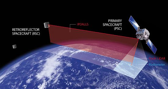
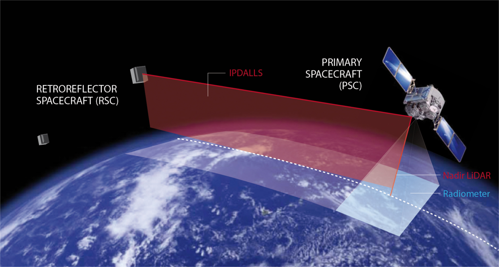
2.4. A New Measurement Technique in Space: Active Limb Sounding

The observational requirements for upper air water vapour, as described above, are challenging to meet. The measurement technique needs to combine very high vertical resolution with a high signal-to-noise ratio for the detection of very low water vapour concentrations. The technique we propose here is an active limb sounding system, based on Integrated Path Differential Absorption (IPDA) LiDAR.

Limb sounding for water vapour is an attractive option because the measurements at high altitudes are not contaminated by the signal from the humid, optically thick troposphere. Current limb sounders (as described above) have resolutions on the order of km in the upper troposphere and above, which is not high enough to resolve the strong vertical gradients in water vapour around the tropopause. Solar occultation techniques, with larger radiative flux densities to analyze, have limited measurement opportunities per orbit. By moving to an active technique, not only can this resolution be improved but the threshold of detection should be lowered, leading to greater sensitivity and a better characterization of the low concentrations of water vapour in the UTLS and above.

The concept of hard target Integrated Path Differential Absorption (IPDA) LiDAR has been around for several decades. Recent studies into spaceborne instruments for trace greenhouse gas detection propose solid ground and cloud surfaces for the reflection of a nadir-emitted pulse [33]. Along with the difficulty of estimating the differential reflectivity over heterogeneous surface types, the signal-to-noise ratio (SNR) of such an instrument will be severely affected by overall low ratios of backscattered radiation and by speckle noise from interference originating at an uneven ground surface. The technique itself is also ill-suited for exploiting the ranging or profiling advantages of a standard LiDAR system, especially above the middle troposphere.

Differential Optical Absorption Spectroscopy (DOAS) is one of the most extensively applied methods for measuring trace species in the open atmosphere [34], producing total path measurements of chemical components from simultaneous observations of spectrally resolved electromagnetic radiation. The technique for the retrieval of multiple species path-integrated number densities has been pioneered amongst others by Platt et al. [35] in the form of long-path DOAS measurements with an active continuous light source, though common passive configurations use natural light as the source, either from direct solar or stellar radiation or from diffuse sunlight. Active long path systems have been proposed both as monostatic and bistatic designs. Monostatic systems use a collocated transmitter and receiver and rely on arrays of retroreflectors from which light is picked up by a telescope, while a bistatic system has a separate transmitter and receiver. Optimal design considerations are discussed in [36].

Since DOAS relies on continuous spectra, laser sources are not common in active set-ups. Nevertheless, an obvious advantage of a laser source is the concentration of the radiant energy within a narrow spectral band and limited beam divergence, albeit at the expense of spectral coverage. A further advantage of targeting only a few selected wavelengths is the possibility to implement significantly higher gain detectors with high quantum efficiency and low noise levels.

For accurate measurements of water vapour, we propose a differential absorption system utilizing elastic backscatter and integrated path LiDAR, centred on wavelength λ_on, an isolated vapour absorption feature in the near infrared, compared to a nearby off-peak λ_off. Integrated absorption of λ_on over the limb path offers a much higher sensitivity (at the expense of spatial resolution) and increases the dynamic range of vapour detection. The selection of the wavelength pairs remains a trade-off between higher accuracy and sensitivity with larger differential absorption cross sections, minimization of systematic errors through smaller wavelength differences and avoidance of absorption bands corresponding to other gases, and finally depends on the frequencies that can be generated by available laser sources [37].

Extinction measurements from such a system would also allow the detection of very low concentrations of stratospheric aerosol, which are difficult to obtain from a conventional nadir backscatter LiDAR measurement alone, and is therefore outside the capability of the CALIPSO mission [38]. Rayleigh and Mie scattering maintain the polarization ratio within a 2%–3% limit, whilst non-spherical particles or multiple scattering may induce some degree of depolarization [39]. This ratio could be used to determine particle shape, phase or multiple scattering, with particularly high values in the case of cirrus clouds with small optical depths, due to particles such as crystallites or hexagonal ice crystals [40], even if it may only be directly relevant for the nadir backscatter signal.

A similar novel active limb-sounding technique has been proposed to ESA [41] as part of the ACCURATE mission (Atmospheric Climate and Chemistry in the UTLS Region and climate Trends Explorer). The mission aims to retrieve atmospheric constituents and line-of-sight winds from occultation measurements between two low earth orbit (LEO) platforms using active microwave and IR signals. In considering the original ACCURATE proposal, the ESA committee noted the mission’s potential for high vertical accuracy, global coverage and good absolute calibration. The Alpbach summer school team arrived at the active limb sounding concept independently, but it is these characteristics that we also wish to exploit, with a focus on water vapour in the UTLS and above.

3. Mission Overview

3.1. Instruments

We propose a novel approach which combines in a single instrument a water vapour Differential Absorption LiDAR (DIAL) in nadir-viewing mode [4,42] with a monostatic IPDA LiDAR in limb sounding by occultation geometry (“IPDALLS”). Looking through the limb of the atmosphere, the IPDALLS system will sample the atmosphere at high vertical resolution with a long integration path. Several wavelength pairs with varying online absorption cross sections will be used to increase the observations’ dynamic range within the UTLS and above. Measurements in this region were beyond the scope of the WALES candidate explorer mission [4], hence this new concept would lead to a more complete and accurate characterization of the water vapour profile. A secondary payload of a medium spatial resolution multispectral radiometric imager would allow wide-swath cloud and aerosol imaging.

The IPDALLS system could be implemented with a bistatic instrument, where transmitter and receiver are on separate platforms. This is the configuration proposed for the ACCURATE mission. However, since two satellites in prograde and retrograde orbits within the same orbital plane could generate at the most four occultations per revolution, the basis of our mission concept is rather a monostatic transmitter-receiver spacecraft flown in formation with multiple spaceborne retroreflectors. An image of the mission concept is shown in Figure 1.

The nadir LiDAR will provide range-resolved vertical profiles of water vapour and aerosols, as proposed for the WALES mission, albeit at slightly relaxed requirements, as the signal will not have to penetrate into the optically thick lower troposphere. The same (or a redundant) transmitting and the same receiving units are used for the limb IPDA LiDAR (see Sections 3.3 and 5.1 for proposed operation and instrument design, respectively). Even if the IPDALLS system, by its implementation, will in principle provide range-gated water vapour and aerosol data in addition to the integrated values, in practice, we estimate that any molecular backscatter signals will probably remain undetectable over the large limb distances involved.

Synergistic data processing—nadir-limb matching—will allow for the simultaneous exploitation of the high along-track resolution of the range-resolved nadir signal with the enhanced sensitivity of a path-integrated measurement from the IPDALLS system. The latter shall also improve the relatively poor vertical resolution that could be achieved with a nadir DIAL signal alone when operating in upper atmospheric regions characterized by low backscatter coefficients. The proposed resolution and sensitivity improvement through the use of multiple observation methods is conceptually similar to panchromatic sharpening of multispectral imagery.

By design, the multiple-wavelength bidirectional LiDAR instrument, core element of the mission’s payload, will emit pulses at water-vapour absorption line-specific wavelengths for the DIAL retrieval. According to studies summarized in [42], three distinct water vapour absorption bands are required for probing the entire atmospheric column from the boundary layer up to the lowermost stratosphere (see Section 5), in addition to a reference offline wavelength in the wing of the absorption spectrum. The four wavelengths used in the WALES proposal were λ_on1 = 935.6845 nm, λ_on2 = 935.5611 nm, λ_on3 = 935.9065 nm, λ_off = 935.4122 nm. In this preliminary study, we find that the same number of wavelengths is required for long path integrated limb sounding from the upper troposphere upwards, and we retain these four wavelengths as a starting point for the performance assessment, even if a posterior optimization study may well lead to a more favourable selection. See Section 4 for more detailed discussion and calculations.

The pump laser’s first (1,064 nm) and second (532 nm) harmonic wavelengths will also be used for retrieval of atmospheric aerosol loading, via backscatter and extinction measurements from the elastic backscatter and retroreflected signals at these two widely spaced laser wavelengths. A measurement of the depolarization ratio will also be made for aerosol characterization.

Inevitably, the presence of clouds will limit the number of IPDALLS measurements, as the technique can only be applied above cloud top height, below which the optical link between the instrument and retroreflector will be lost. However, in its function as an aerosol elastic backscatter LiDAR and due to its bidirectional viewing geometry, in these situations the system will act as a combined range-gated nadir-limb ceilometer, especially for thin high altitude cloud decks with a sufficiently large horizontal spread. It will thus provide information on the vertical extent of high altitude, optically thin translucent clouds, such as (contrail) cirrus, polar stratospheric and noctilucent clouds. Given a typical cirrus cloud thickness on the order of 1–2 km, achieving a high vertical resolution from the combined data is crucial.

A fairly conventional radiometric imager will be used for the retrieval of cloud macro- and microphysical properties at cloud-resolving scale, following the operational method of Rosenfeld and Lensky [43]. Clouds are detected using the brightness temperature difference between visible and thermal infrared channels; cirrus ice clouds and water clouds can be distinguished by the brightness temperature difference between particular thermal infrared channels, which can also be used for the retrieval of cloud top temperatures (and heights).

The radiative impact of cirrus clouds is dependent on certain physical cloud parameters: effective particle radius (R_e), ice water path (IWP), the optical depth (τ), and the vertical position of the cloud, manifested in its cloud top temperature and cloud top height. The radiometer spectral bands have been chosen to be sensitive to these parameters. The visible (VIS) and short-wave infrared (SWIR) bands (0.66 μm and 1.66 μm) are highly sensitive to R_e, IWP and thus τ. The 10.8 μm and the 12.0 μm bands are also sensitive to the same parameters, but need to be combined with additional bands for accurate results: VIS/SWIR bands during daytime and the 3.9 μm mid-infrared (MIR) band during night. The thermal infrared (TIR) bands are sensitive to cloud top temperature and height [44]. The five bands specified above are the minimum requirements to recover the desired cloud parameters. Additionally, two SWIR bands, 1.38 μm and 1.24 μm, are incorporated into the radiometer design. The 1.38 μm band enables to detect upper level cirrus clouds, especially over land [45]. Furthermore, the ratio of the 1.38 μm band over the 1.24 μm band is very effective in discriminating upper level cirrus clouds from the lower level aerosols and dust [46]. The horizontal distribution of column integrated water vapour will be retrieved from a further, dedicated band at 6.3 μm, and will be useful for the context interpretation of the nadir LiDAR data and their cross-validation.

3.2. Orbit Specification

The appropriate orbit for this mission concept is a circular low Earth orbit (LEO). Crucial to the implementation is a phased homogeneous constellation of retroreflectors on board multiple microsatellites, counter-rotating with respect to the monostatic active spacecraft, and in the same orbital plane. A single plane is required for the occultation geometry, to achieve collocated nadir and limb measurements and for relaxed requirements to the pointing and tracking system described in Section 5.4.

Relative precession between both orbits must be avoided; for a mission which requires global coverage, this can only be achieved with satellites in a polar orbit. Furthermore, the altitudes of the primary and retroreflector spacecraft should be close, to ensure that the descent of the tangent point throughout the atmosphere is as close to vertical as possible, though a minimum altitude separation of 20 km is recommended to minimize collision risks [47]. We suggest that the constellation of retroreflector spacecraft is injected onto the lower orbit to avoid collision with the primary satellite in case of orbit maintenance problems for the microsatellites.

Five retroreflector spacecraft on a 550 km LEO (270° inclination, 5,738.8 s period) in combination with a 582 km LEO (90° inclination, 5,778.6 s period) for the primary satellite have been identified to provide an optimal configuration. This involved a trade-off study between the number of occultations required, the measurement sequence timing, the amount of atmospheric drag and implications for orbit maintenance, as well as considerations about the nadir LiDAR SNR, which decreases with increasing path length (altitude). The altitude has been set to produce a 10 day return period of the ground track. Active orbit control will guarantee high accuracy inclination maintenance and prevent relative drift of the orbital planes (see Section 5.5 for more details).

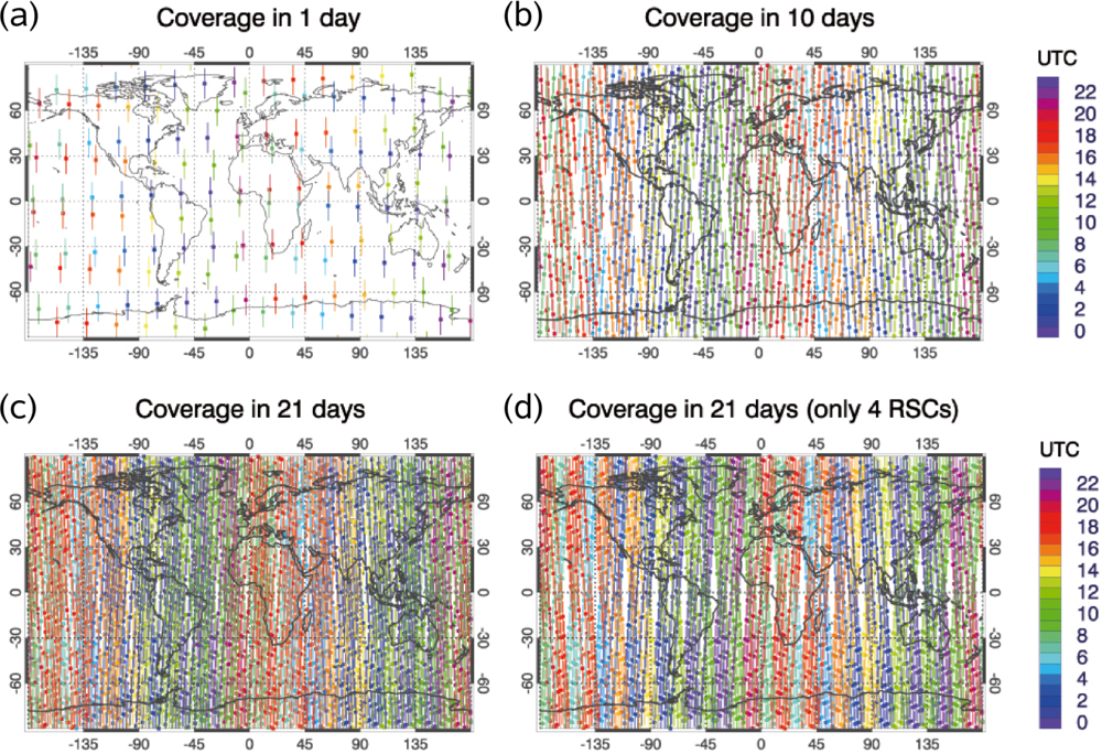
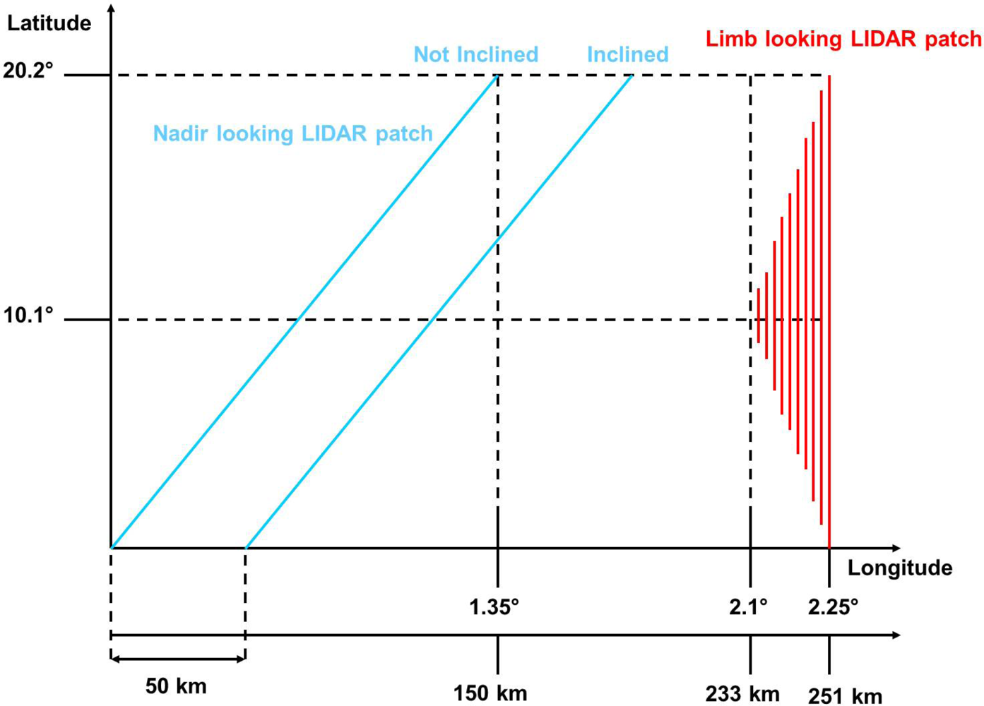
3.3. Measurement Sequence and Coverage

A typical measurement sequence for the nadir LiDAR and limb sounding observations lasts for a total of 540.6 seconds; this is depicted in Figure 2. The sequence comprises the time for nadir LiDAR observations, tracking and locking of a retroreflector, calibration of the IPDALLS system and finally the limb measurement itself. The sequence is designed so that the nadir and limb measurements are roughly collocated (within 200 km; see Figure 4 and the discussion thereof, below).

In order not to overstretch power and heat evacuation requirements and to maximize the outgoing pulse energy, the nadir and limb instruments are powered sequentially. The sequence begins at time t₀ with the nadir LiDAR operating at a nominal pulse repetition frequency (PRF) of 25 Hz for 324 s, covering a ground track of 2,244 km, the midpoint of which corresponds to the tangent point of the following limb sounding and approximately to the orbital crossing of the primary and secondary spacecraft. At time t₁ a search and lock procedure (described in Section 5.4) is initiated to establish the optical link between the instrument and the retroreflector; this optical communication procedure can take no longer than 122 s. Once the link is established, it will be maintained by an internal tracking mechanism within the IPDALLS instrument. The limb occultation measurement starts at time t₂ with ‘free space’ calibration measurements taken from a height of 250 km down to 100 km (t₃). Scientific data is gathered for 35 s between t₃ and t₄, from a height of 100 km down to ground level, although in practice the link will be terminated at optically thick cloud top height (estimated between 5 and 15 km according to the latitude and season), and data may not all be downlinked due to communication constraints. During the idle time of 35 s between limb sounding termination and the next collocated nadir sequence, the system will resume and dwell in nadir sounding mode, thereby maintaining a continuous laser operation to increase transmitter lifetime, and providing further science data.

Figure 3(a) shows the simulated coverage for one day of measurements with five retroreflectors, with the measurement tracks coloured according to time of day (UTC). Observations are global, with the largest orbit step or measurement gap of about 2500 km around the equator, and highest sampling density over the poles (although a certain proportion of these will be lost when the instrument is pointing directly at the Sun). Figure 3(b) shows the coverage over 10 days, and Figure 3(c) over 21 days of operations. Three weeks’ sampling produces almost global coverage, with the largest gaps at the equator reduced to around 500 km, and simultaneously the sub-diurnal sampling has been improved. Coverage will always be limited by the narrow ground track of the LiDAR system. In the case of the loss of one retroreflector, global coverage after 21 days is not significantly affected (Figure 3(d)). The largest impact is over the tropics, although gaps are still less than 800 km, but coverage remains excellent at mid-latitudes and over the poles. The wider swath of the multispectral radiometric imager leads to a much swifter global coverage by the passive instrument.

A limitation of the prescribed polar orbit is the convoluted sampling of the diurnal and seasonal, or intra-annual, water vapour cycles for any given location. In other words a full 24-h cycle will only be sampled over the course of a year. This is not ideal for a tracer that is highly variable both in space and in time; however, for a given latitude belt, at least two diurnal observations will be available within a narrow zonal region.

Because of the Earth’s rotation between times t₀ and t₃, the measurements taken by the nadir and limb looking LiDARs will not exactly cover the same track. However, the nadir instrument is pointing slightly cross-track or off-nadir to avoid specular reflection, which mitigates this effect. Furthermore, collocation should be defined as a function of the characteristic spatial scales of variability of the observed phenomenon. For tropopause folds and tropical pumping of water vapour into the UTLS, this characteristic scale is of the order of 100 km. Our analysis (shown in Figure 4) produced a typical measurement track offset at the equator at ground level (the worst case) of between 33 and 200 km for an off-nadir angle of 5°.

3.4. Data Retrieval and Use

Observations from this novel system are designed to deliver higher resolution and higher sensitivity water vapour measurements than currently exist for the UTLS and above. It will help to quantify and understand the differences between current water vapour measurements, and will provide collocated active and passive measurements of water vapour, clouds and aerosol for process studies. Full exploitation of the potential of this combination of measurements will require further research, but much progress has already been made in understanding and assimilating limb observations.

Inversion algorithms for the nadir water vapour and aerosol elastic backscatter LiDAR will follow standard procedures adopted for DIAL measurements. The inversion of an integrated path DIAL signal is conceptually rather straightforward, though specific considerations for an occultation geometry will complicate the picture somewhat: chromatic ray bending, refractive dilution and scintillations (see [30] and references therein, for the GOMOS stellar occultation measurements), a number of considerations related to the use of narrow absorption lines (see [48] and references therein, for a water vapour DIAL system), as well as background radiance from sunlight scattering and spontaneous emission (e.g., from auroras). We expect that well-established retrieval approaches for limb sounding systems, such as ‘onion peeling’ implemented, e.g., for SCIAMACHY solar occultations [28] will be adapted for this system. These algorithms require the use of a reference atmosphere, and the quality of the results will depend on the appropriateness of that reference. However, Noel et al. [28] find that this dependence is greatest at low altitudes and is negligible at an altitude of 35 km. Long path inhomogeneities will need to be deconvolved from the limb measurements.

With a nominal PRF of 25 Hz for the limb sounding, we avoid signal ambiguities at the maximum path length between the instrument and the retroreflector (∼5,500 km). This means that the previous pulse returns before the following is emitted. At a vertical descent rate of the optical link through the atmosphere of approximately 2.8 km/s, the vertical sampling resolution is therefore constrained to roughly 110 m. Single signals may need to be integrated to increase the SNR, which is typically proportional to the square root of the number of shots, and the actual vertical resolution will be degraded accordingly. We expect to find single shot SNRs from the reflected pulse returns large enough to make large averaging sets unnecessary, though this has yet to be confirmed by a detailed end-to-end simulation (see Section 4 for the preliminary calculations). In addition, with every pulse or burst, 4 DIAL wavelengths are emitted, yielding three pairs for averaging, even if two of them will generally be inadequate for the water vapour concentration at a given altitude.

Forward radiative transfer modelling of brightness temperatures and reflectance as a function of cloud parameters across the relevant wavelengths will be used to generate look-up tables for the exploitation of the radiometer data. By matching the observed data to the look-up table values, users can recover the cloud properties.

Benefits of this novel system are likely to come from the improvement of model routines and parameterizations through process studies of clouds and convection. Assimilation of high resolution, accurate water vapour measurements within models would lead to improved water vapour convergence estimates [4]. It would also provide a framework for enhanced information extraction and the interpretation of dynamic features of the atmosphere occurring within the UTLS. This is particularly relevant for creating climatologies of the tropopause structure, including the identification of stratosphere-troposphere exchange events and tropopause folds, and to resolve structures and finer-scale fluxes in the UTLS and lower stratosphere, such as the polar vortex or water vapour fluxes above the top of deep convective clouds. Such assimilation systems are likely to operate on finer resolutions than are currently the state-of-the-art, which will make corresponding high resolution measurements ever more necessary.

4. Preliminary Performance Considerations for IPDALLS

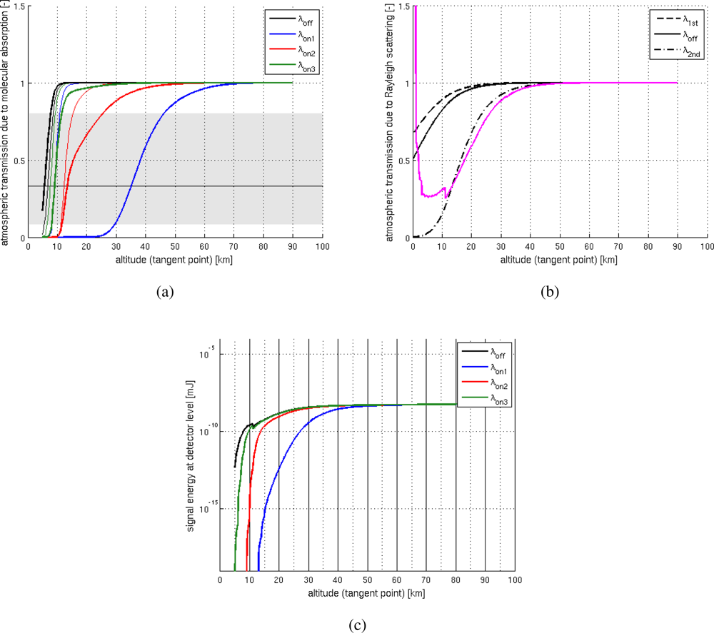
4.1. First Order Estimation of the Link Budget and Measurement Accuracy

Here we present a preliminary feasibility study of the IPDALLS concept with respect to our primary mission objective, i.e., the profiling of water vapour in the UTLS and above, using a model developed for rough systems trade-offs. In due course, detailed instrument performance end-to-end simulations and corresponding sensitivity studies, noise and error evaluations would be required, as outlined, e.g., in [33,48–52] for similarly operating payloads.

For a system relying on wavelength pairs with extremely narrow spectral separation, pressure and Doppler broadening of the absorption lines, determining the Voigt line profile, as well as water vapour self-broadening, will become very relevant. Consequently, absorption cross sections will need to be calculated as a function of pressure and temperature, or altitude (as in Figure 5), and corresponding atmospheric profiles assumed, retrieved or modelled as a preliminary step in a retrieval algorithm. Furthermore, the Doppler shifts induced by the diverging spacecraft, different for the forward and the backward paths, will need to be accounted for in the estimation of the absorption cross sections. For these preliminary calculations, we assumed online wavelengths centred on the absorption peaks of motionless molecules at the tangent point and on the forward path, which have thus been previously generated at a slightly higher frequency by the receding transmitter. The Doppler shift induced by the receding retroreflector, and experienced by the same molecules on the backward path, corresponds to an average beat frequency of −14.9 GHz or a red-shift of 43.6 pm. In general, this makes the atmosphere more transparent on the backward path, even if the shifted λ_on2 now resides in the highly sensitive region of a wing’s inflection point, which may introduce a potential source of uncertainty. The equations and methodology used to estimate the performance of the IPDALLS concept are described in Appendix, and an abbreviated set of baseline instrument parameters is given in

Table 1. Specification of instrument components used in the preliminary performance calculations.

Instrument key parameter	Unit	Value	Comment/Origin
Transmitter
Pulse energy @ 935 nm	[mJ]	75	aligned with [4]
Effective pulse length (τL)	[ns]	75	aligned with [33]
Laser beam divergence (θl)	[μrad]	15	system preliminary design (minimize beam broadening)
Receiver
Telescope diameter (Drec)	[m]	0.50	system preliminary design
Telescope field-of-view (FOVrec)	[μrad]	280	system preliminary design, aligned with [33]
System optical efficiency (ηsys)	[-]	0.40	estimate, aligned with [33]
Detector (Excelitas/PerkinElmer Si APD C30954E-DTC)
Nominal gain (M)	[-]	120	product specification
Responsivity @ 900 nm (R)	[A/W]	75	spec, unit gain responsivity estimated as R0 = R/M
Maximum peak rating	[mA]	10	product specification
Surface dark current @ 22 °C (Ids)	[nA]	50	value obtained from manufacturer
Bulk dark current @ 22 °C (Idb)	[pA]	200	value obtained from manufacturer (range 1–200)
Retroreflector
Effective reflector area (Aref)	[m2]	0.20	system preliminary design
Reflector efficiency (ηref)	[-]	0.80	estimate
Reflector beam divergence (θr)	[μrad]	40	estimate, larger than twice the laser beam divergence

.

Figure 6(a,b) shows the various transmission profiles in limb sounding geometry for a standard mid-latitude daytime atmospheric profile due to molecular absorption and scattering, respectively. Molecular absorption (in particular due to water vapour) was calculated using the MIPAS Reference Forward Model (RFM, see Appendix) in a standard mid-latitude daytime atmospheric profile, while scattering was calculated with the 1976 US Standard Atmosphere. The differing absorption of the various wavelengths at a given tangent point height is evident, as is the necessity to use several wavelength pairs (with the same reference offline wavelength) to probe different altitudes, since wavelengths with strong absorption coefficients, and hence good sensitivity at heights where water vapour concentrations are low, are completely absorbed in the lower atmospheric layers. Scattering is essentially the same at the on- and offline wavelengths, which is one advantage of this differential absorption technique. A retrieval of atmospheric aerosol, one of the secondary mission objectives, would exploit scattering at widely spaced wavelengths. Figure 6(b) shows that below 10 km, very little signal is received from the 532 nm harmonic when considering molecular scattering alone (i.e., before considering the effect of aerosol), so synergistic limb-nadir aerosol retrieval would likely be constrained to the stratosphere, where ozone absorption will need to be accounted for. Also plotted is the refractive dilution factor (see, e.g., Dalaudier et al. [54]), which becomes increasingly relevant for signal attenuation within the UTLS and below. The kink at around 10 km is due to the strong refractive index change at the level of the tropopause. The irregularities and increase of the factor below about 5 km are related to a refractivity decrease in the moist lower troposphere, due to high water vapour contents, and this region is excluded from our performance simulations.

A simplified power budget is used to estimate the returned signal energy for the limb sounding measurements, and corresponding profiles are shown in Figure 6(c). Losses are assumed to be mainly due to geometric beam broadening, molecular absorption and scattering, retroreflector and receiver efficiency, continuous as well as turbulent refractive effects and aerosol extinction, the last two of which we have not considered in this study. In practice, many further noise and error sources have to be considered, and a good account of key issues affecting the SNR of a nadir IPDA LiDAR is given in [33]. In this paper, we will for simplicity only consider the carrier-to-noise ratio (CNR) as a means to estimate measurement sensitivity with respect to the water vapour optical depth and expected random errors.

To achieve a high CNR, we need to maximize the light throughput of the transmitted beam, by using a high power source with small beam divergence. We simultaneously need to minimize scattered light, by using a high focal number telescope to reduce the field-of-view (FOV). The solar background radiance, the standard limb passive DOAS signal, will be considerable for any daytime measurements in the near-infrared and at visible wavelengths. If scattered sunlight were on the same order of magnitude as the received laser signal, this would considerably limit our observation capabilities. Sugimoto et al. [55], on the other hand, report no significant influence of sunlight in laser ground-space absorption measurements in IR wavelengths. Exposure to direct sunlight has not been considered, since it is likely to damage the detector and needs to be avoided.

Figure 7(a) shows the contribution of the various sources of noise to the total detector noise current for the on- and offline wavelengths: signal shot noise, Rayleigh-scattered solar background in the baseline case of 0° azimuth and 60° zenith solar angles with respect to the occultation plane and detector dark current noise from surface and bulk origins. The maximum signal photocurrent of 6 mA at the top of the atmosphere (TOA) falls well within the maximum peak rating of the detector (Table 1).

Figure 7(b) shows the CNR with altitude: the potential of the IPDALLS technique is evident from the very high CNRs achieved throughout the stratosphere and into the tropopause layer, with TOA peak ratios on the order of 700. Similar values have recently been reported for a comparable mission concept described in [41]. The kink around the tropopause originates from the refractive dilution.

Above roughly 25 km, where atmospheric transmission is high, the CNR for all wavelengths is clearly signal noise power limited (see [56]). Consequently, few improvements can be expected from reducing detector noise or telescope FOV, and the stringent requirements with respect to the latter could be relaxed, making search and tracking easier. The same holds for the lower atmospheric layers, where the signal shot noise remains consistently larger than the background and detector noise at the online wavelength corresponding to the relevant height range, although scintillation variance is likely to lie above the shot noise. Equally, the range of possible occultations could be increased to include configurations with higher solar zenith angles than the baseline. Note however that neither the background from auroras, stellar radiation and non-Rayleigh scattering, nor interference speckle have been considered, and that the actual received signal power and shot noise are likely to be lower due to larger optical depths in the real atmosphere and less favourable parameters in the real system. Also, the full assembly of detector and amplification circuit would need to be considered to evaluate the real optical receiver noise current.

Figure 7(c) shows the relative random error at maximum sampling resolution for single shot measurements. For each wavelength pair, the random error increases at low altitude because of a weak CNR and at high altitude because of decreasing differential absorption. Over the entire measurement range defined in the mission objectives, the modelled random error on the two-way path-averaged water vapour optical depth varies between 0.2% and 3%, with a significant contribution of refractive dilution to the error within the UTLS. Optimizing the choice of wavelengths may still improve these results and narrow the current gaps between the optimal retrieval ranges. Since the model atmosphere used to simulate transmission after molecular absorption held about 6 ppmv of water vapour towards the upper altitudes of 45 to 50 km (not shown), we hypothesize that significantly lower water vapour concentrations can be detected at lower heights where the effective absorption path increases. However, more advanced modelling and system definitions would be required to translate the modelled random error into errors on mass mixing ratios and to account for systematic errors and additional factors influencing the random error.

4.2. Potential Performance Limitations

The results presented above have been obtained without considering the turbulent nature of the atmosphere and related multiple diffraction effects, which arise in addition to the continuous refractive dilution and chromatic refraction. Random anisotropic and isotropic irregularities in upper air density, originating from internal gravity waves, wave breaking, wind shear and other instabilities, result in inhomogeneity of the refractive index which leads to temporal and spatial fluctuations in the recorded intensity of radiant energy: scintillations. Scintillations have been successfully exploited in stellar occultation for gathering data on atmospheric turbulent dynamics (e.g., [57–59]), however they severely affect the absorption measurements of the GOMOS instrument (e.g., [60]), the most relevant comparable payload on orbit, and may be even more detrimental for laser (coherent) radiative transfer due to the generation of speckle patterns.

The only analogue to our proposed measurement technique is an inter-orbit optical communications experiment between a geostationary and a LEO platform, which maintained a narrow-beam link through the atmosphere during an occultation event [61,62]. In this case, the combined action of a smaller continuous wave laser divergence and the very long distance to the geostationary orbit made the technique more susceptible to angular beam deflections (wander) than the one described in this paper. Both terminals experienced strong fluctuations of the received power, a non-monotonic decrease of the normalized intensity log-normal probability density mode from about 50–40 km downwards, first detector saturation due to refractive lens effects at about 35 km, and a termination of the optical link in the best case at 15 km.

For GOMOS retrieval corrections [60], this steady decline of the average power has been factored into the total atmospheric transmission as an altitude-dependent transmittance, in which refractive dilution is modulated by scintillation estimated from measured intensity fluctuations. The average decrease in signal strength is simultaneously accompanied by temporal amplitude fluctuations due to scintillations which often exceed the GOMOS instrumental noise, hence impacting the SNR and therefore the measurement error in a twofold way. According to the available scintillation measurements, the scintillation variance is saturated below 25–30 km at a root-mean-square level of about 100% of the mean signal. Such a level of scintillation variance within the UTLS can also be expected for the IPDALLS principle.

Even if two spectrally adjacent channels are affected by turbulence in virtually the same way, this may not improve the single shot SNR in the individual channels, and scintillations will still degrade the measurement accuracy. Since wavelength separation for water vapour is very small (less than 0.06%), the light at the different wavelengths travels essentially through the same air density irregularities, if emitted simultaneously. In combination with short laser pulses, this allows us to expect that the impact of scintillations on differential absorption in water vapour channels is very small. According to simulations for ACCURATE [63,64], we can expect the root-mean-square error in differential transmission due to scintillations to remain less than 1% down to 5–10 km for the proposed system.

On the other hand, MacKerrow et al. [65] point out that the correlation between multi-chromatic signal fluctuations is minimal when speckle dominates over other sources of noise, the speckle pattern between different wavelengths itself is decorrelated, and the mean number of integrated speckles per pulse is small, which can be expected in classic hard target low-divergence LiDAR systems. Pure retroreflection speckle has been observed during laser ranging due to the use of reflector arrays [66], but avoided by design for absorption measurements through the use of a single cube-corner retroreflector [55], such as proposed in our preliminary design. Turbulent refraction will also degenerate an initially Gaussian beam profile into spatial intensity fluctuations in the incident wave plane, characterized by a spatial correlation scale, and leading to further potential signal loss, even if MacKerrow et al. [65] are referring to interference generated during the reflection of coherent light off a rough Lambertian target. This is of less concern to the technique described in this paper, and results off a small (essentially point) retroreflector showed a much higher bichromatic cross-correlation (0.87), albeit with relatively high variance [67]. For a retroreflector and a receiving telescope of finite apertures, the possibility of integrating over such a speckle structure or individual cells will need to be accounted for [66]. For the total power not to be fluctuating, the aperture sizes would need to be larger than the spatial correlation scale [68], which is not satisfied with the current design specifications. In particular, if the radius of a single (point) retroreflector is smaller than the intensity spatial correlation scale, fluctuations in the reflected flux will not be averaged by a receiving aperture of arbitrary size, though a larger telescope diameter would still reduce the signal variance.

Ehret et al. [33] show for a rough target IPDA LiDAR that speckle has a large potential to severely degrade the final SNR, and all of the above will need to be considered in a much more detailed analysis of the expected performance of our system, and validated experimentally. We can already note, however, that we expect strong constraints on the optimistic results presented in the previous section. The GOMOS transmission spectra retrievals are corrected for by anisotropic scintillation measurements from the fast photometer [60]; we expect to realize similar corrections by introducing scintillation quantification using the continuous-wave high-divergence IR beacon laser potentially required by the PAT system (see Figure 8), which would also provide the potential for gathering further science data.

5. Mission Technical Implementation

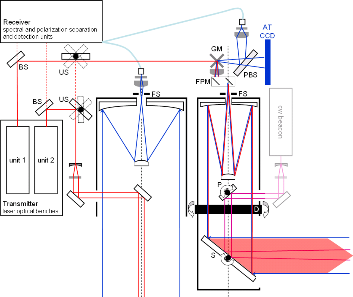
5.1. Payload Design: IPDALLS System and nadir LiDAR

Based on the aforementioned measurement configuration, the mission’s primary payload comprises a multi-wavelength bidirectional transmitting system, receiving optics, a spectral separation and detection unit, a transient recorder data acquisition unit, a control unit and a scanning and tracking facility based on novel (albeit proven) optical communication technology. A simplified conceptual block diagram (Figure 8) illustrates the payload subdivision into nadir and limb pointing instruments.

The transmitter constitutes a critical driver of the overall mission concept. Since the concept draws extensively from the heritage of the WALES mission proposal, and because of necessary further industrial feasibility studies, a detailed description of the laser source is beyond the scope of this study. A comprehensive account on water vapour differential absorption LiDAR transmitter choices can be found in [69]. In addition, retrieving profiles of atmospheric aerosol size distribution, backscatter and extinction coefficients from elastic backscatter LiDAR signals generally relies on at least two widely spaced laser wavelengths and their polarisation.

DLR’s airborne WALES precursor described in [42] uses two Nd:YAG lasers in master oscillator/power amplifier configuration. The radiation of the WALES pump lasers is frequency doubled by a second-harmonic generating crystal (532 nm) and then converted to values in the vicinity of 935 nm by an Optical Parameter Oscillator (OPO). The output of the OPO is switched between two wavelengths, using calibrating seed laser diodes that can be tuned over a range of about 1 nm via temperature or current control. In order to provide the four wavelengths that have been used in our preliminary performance studies, two identical chains of lasers and non-linear conversion stages would need to be synchronized in a temporally interleaved fashion, at least during nadir operation.

Industrial research into most mature transmitter options for the spaceborne WALES ESA candidate mission converged however on a high-energy Ti:Sapphire oscillator in a ring cavity configuration, pumped by a frequency-doubled Nd:YAG laser and injected by four tunable seed lasers to set the frequencies [4].

The stringent requirements on frequency stabilisation for water vapour detection, particularly relevant in the stratosphere where absorptions lines are very narrow, can be met by the use of seed lasers used in conjunction with a multi-pass water vapour absorption cell (for reference) and wavemeters. Wirth et al. [42] gives a good overview of techniques implemented for the monitoring and diagnostics of the source’s very high frequency stability and spectral purity (typically >99.9%). A particular challenge of active laser sounding in limb geometry with retroreflection will arise from spacecraft motion-induced Doppler shifts. Doppler shifts can be precisely modelled from orbit geometry and are expected to vary by less than 1 pm over the sounding altitudes range. However, absolute wavelength shifts on the order of 43 pm for diverging spacecraft and extremely narrow water vapour absorption peaks imply that emitted online sounding wavelengths will need to be generated and calibrated outside the actual absorption peaks. Furthermore, wavelengths will be shifted twice, on the forward as well as on the backward path, implying that peak absorption can only occur over one of them and effectively reducing the lower detection limit.

The transmitter’s heat-generating elements are cooled by a heat pipe assembly linked to the primary spacecraft’s temperature control subsystem. Temperature control should provide a stable regime at an equilibrium temperature to minimize thermal stress on the transmitter. As mentioned above, it may be necessary to operate a single transmitter unit continuously and to switch its output between the nadir and limb systems. Switching must be designed to avoid single failure points and to guarantee the maintenance of accurate optical alignments over the mission lifetime. It may also be necessary to implement fully independent redundant transmitter units as back-up in case of premature failure. The use of redundant units must be traded-off against thermal requirements and overall weight and size.

The receiving optics consist of a separate, slightly cross-track off-nadir telescope and a limb telescope. Our preliminary design calculations were based on limb measurements with a 0.5 m diameter telescope, while the required nadir optics were specified with a larger 1 m diameter main mirror, in order to collect sufficient backscatter radiance from the lowermost atmospheric region determined by the mission objectives.

A fine-pointing mechanism within the limb optical path is used for scanning the laser beam within the telescope’s FOV. Before beam collimation of the limb telescope signal, a small proportion of the received power (above 1,000 nm) is projected onto an acquisition and tracking CCD in the image plane, using a beam splitter. This image is used to localize the retroreflecting spacecraft within the telescope’s FOV for a faster and more efficient searching and centralizing procedure. Aside from this, the same spectral separation and detection unit can be used for both nadir and limb instruments (see Figure 8); it may however be preferable to use two different units optimized for their respective sounding principle, providing redundancy and/or limiting signal losses due to beam combining. Since the four water-vapour wavelengths are sent off sequentially, one single gated detector could in theory be used for all of them (see [42]). In practice, the optimal pulse separation time (order of 100 μs) will be much smaller than the maximum return time for spaceborne nadir (order of <4 ms) and limb (order of <40 ms) sounding, which makes wavelength separation or demultiplexing mandatory.

In [4], wavelength separation through Fabry–Pérot etalons tuned to the respective frequencies was proposed, but other spectral separation can be envisaged as well. Individual detectors will be shielded from solar background noise via narrow-band (nominally 1 nm) interferometric filters. Dielectric beam splitters will be used to separate the 1,064 nm first- and the 532 nm second-harmonic channels, for which the depolarization ratio will be analyzed using a polarizing assembly. Low dark current analogue avalanche photodiodes (APDs) are needed for the near-IR channels, whilst photo-multiplier tubes (PMTs) or appropriate (vacuum) APDs will be used for the 532 nm wavelength. Gated diaphragms are used to avoid telescope cross-talk and direct sun exposure. The outgoing pulse is sampled for pulse diagnostic and calibration and transient recorder triggering. Hardware averaging over multiple range-bins or pulses onboard the spacecraft was deemed inappropriate in [4], which will be an important factor to consider when sizing the data downlink.

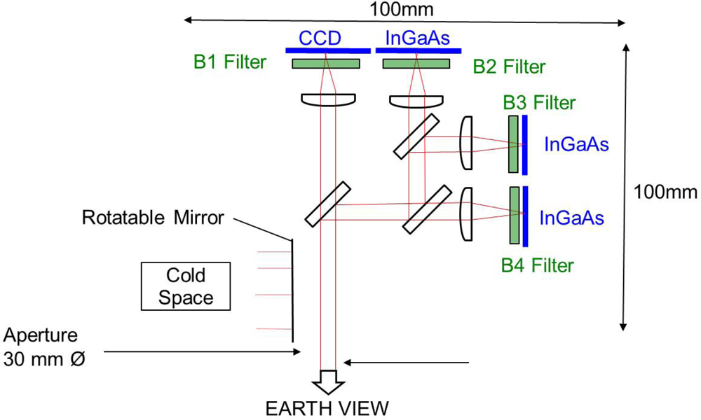
5.2. Payload Design: Radiometer

The radiometer is a fairly conventional design, and consists of two multispectral sensor instruments. The instruments are designed to provide images of the visible and infrared at the chosen wavelengths and bandwidths, with a concept halfway in between AVHRR/3, with which it shares 4 bands, and MODIS, with 7 bands shared. The instrument uses pushbroom scanner technology, in nadir orientation. The 200 m × 200 m resolution requirement is fulfilled by 1 × 2,048 pixel sensors and a nominal dwell period of approximately 26 ms. The detectors are read out five times during the dwell period, to avoid saturation.

Each instrument consists of a single box containing all optical, electronic and mechanical elements. Large radiator areas are available for heat dissipation to provide a stable environment for the VIS/SWIR and the MIR/TIR detectors. The payload will be composed of four units:

• The VIS/SWIR instrument, providing data from four spectral channels (VIS: 0.66 μm, SWIR: 1.24 μm, 1.38 μm and 1.66 μm).
• The MIR/TIR instrument, providing data from four spectral channels (MIR: 3.90 μm and 6.30 μm, TIR: 10.80 μm and 12 μm).
• A common optical bench module that interfaces with the platform. The bench is located outside the main platform structure, with the control unit inside.
• The instrument control unit that drives both the VIS/SWIR and the MIR/TIR instruments.

The VIS/SWIR system optical design is shown in Figure 9. Dichroic splitters can reduce the size of the calibration diffuser by providing a common aperture for all four channels. Since a common entrance pupil (aperture) is necessarily remote from the lenses, we should point out that dichroics tend to decrease the optical system size.

The VIS/SWIR sensors are made of silicon charged coupled detectors (CDDs) and indium-gallium-arsenide (InGaAs) detectors. As the operating temperature of both the CCD and InGaAs detectors fits within the −10 °C to +40 °C interval, copper heat exchangers can provide sufficient thermal control. The Fairchild CCD 143 sensor and SU-LDH-1.7 Linear Digital High speed InGaAs sensor fit the instrument requirements.

A rotatable calibration mirror is used in order to provide views both of Earth (bright source views) and cold space. The bright source is provided by the observation of high level opaque clouds, bright deserts or dark oceans for fulfillment of a calibration accuracy better than 5%. Using a range of bright sources allows coverage of the full dynamic range of the instrument. An on-board algorithm provides the calibration target characterization [71].

The MIR/TIR optical system design is shown in Figure 10. Using three separate detectors with independent optics would require three relatively large apertures, and would also have a fairly severe impact on the size of the external calibration hardware. A single aperture and a single detector is therefore preferred, partly for control of system size, but also since a single calibration source and a single detector will likely provide optimum inter-channel relative accuracy. For the TIR, we introduce the dichroics near an intermediate image formed at relatively low aperture, where we have placed the two TIR filters. After exiting the filters, the large intermediate image is directed onto the detector by a relay lens.

The MIR/TIR sensors are made of mercury-cadmium-telluride (HgCdTe). The TIR instrument uses a Stirling cycle cooler for maintaining the detectors temperature at 77 K, which provides the required radiometric resolution. A slight modification to the 2,048 × 2,048 pixel Teledyne HAWAII-2RG, used in astrophysics, should suit the instrument requirements.

For MIR/TIR calibration a rotatable mirror is used in order to provide views of the Earth, of cold space and of a bright black body. The last two views provide the two known radiance levels that are required for absolute calibration of all MIR/TIR channels. The mirror is used at the same angle of incidence for cold space and Earth views, so that it has the same emissivity in these two configurations, providing a very good zero radiance reference. Edge structures on the mirror are used to block the cold space aperture during Earth view. The warm black body is a deep-cavity black body, with an emissivity that will always be very close to unity. The black body temperature will be monitored precisely and provide a calibration accuracy better than 1 K.

5.3. Spacecraft Design: Mass and Power Budgets

The overall size of the primary spacecraft will be in the range of 3.5 m × 2.5 m × 2.5 m and will be shaped by the limb and nadir telescopes, the optical benches, solar arrays and radiators. It will have a dry mass of roughly 3,000 kg. In this configuration it can be launched from a Soyuz launcher. The payload is estimated to consume an average of 1,500 W, with the spacecraft bus requiring around 700 W. To supply the energy for the subsystems and the payload, and to charge the batteries for the eclipse time, a solar array of 17 m² will be required. It will be panel-mounted to accommodate the large area and optimize the Sun incidence angle by two-axis Sun tracking.

To maintain the payload and the primary spacecraft subsystems within their operating temperature ranges, two radiators with an area of 5.8 m² each are attached at two sides of the spacecraft to dissipate heat. Louvers ensure that one radiator will always face deep space, while they are closed when exposed to direct sunlight. Heat pipes will transport the heat to the radiators, and to the heaters for eclipse time, and in emergency cases will sustain a minimum temperature for the payload and the battery.

The role of the retroreflector spacecraft is to reflect the laser pulses back to the primary spacecraft. The design performance directly determines the quality of the IPDALLS measurement. Several options for the design of the retroreflector spacecraft were studied.

Initially, completely passive satellites with multiple retroreflective surfaces were considered, similar to those flown in the LAGEOS mission [72]. Several issues, such as orbit deterioration, lack of control and inability to de-orbit in a controlled manner, caused this idea to be rejected and an active retroreflector was deemed necessary. Active spherical retroreflector satellites, having multiple retroreflective surfaces but with added orbit control, were then considered. This idea was eventually dismissed because of launcher housing complexity and difficulty to manufacture. In addition, the multiple retroreflective surfaces may have caused speckle noise distortion of the beam signal and point-ahead-angle issues [55].

The final retroreflector spacecraft consists of a microsatellite with attitude and orbit control (0.65 m × 0.65 m × 0.8 m) carrying a single corner cube retroreflector with a diameter of 0.5 m and an effective reflective area of 0.2 m². The mass and power budget of both the primary spacecraft and a retroreflector spacecraft are shown in

Table 2. Mass and power budgets for the primary and the retroreflector spacecraft.

	Primary Spacecraft		Retroreflector Spacecraft
Component	Mass (kg)	Power (W)	Mass (kg)	Power (W)
Payload	1,100	1,500	44	–
Spacecraft Bus	1,280	700	45	16
Margin	600	530	21	4
Spacecraft Dry Mass	2,980	–	110	–
Propellant	280	–	16	–
Total	3,260	2,730	126	20

.

5.4. Spacecraft Tracking

Laser ranging from available ground station networks is performed continuously to accurately track the retroreflector spacecraft. This information is used for updating contact schedules with the primary spacecraft. The retroreflector spacecraft will be positioned in the direction of the primary spacecraft using its attitude control system and positioning data. Retroreflector spacecraft tracking, by the primary spacecraft, commences when the nadir measurements have been completed and continue until the retroreflector spacecraft disappears behind the Earth horizon, approximately 215 seconds later (as shown in Figure 2). The primary spacecraft will receive the positional data of the retroreflector spacecraft to within 0.1 m (via the ground station) and GPS data for its own position.

The primary spacecraft performs a search for the retroreflector spacecraft (using its scheduling data) to establish the initial Line of Sight (LOS). The PAT system may incorporate a separate, low-power, high-divergence laser to perform broad search pattern techniques until a signal is received, at which time, measurement can commence using the low-divergence laser. A small proportion of the received power (above 1000 nm) is used to localize the retroreflecting spacecraft within the telescopes FOV for a fast, closed loop efficient tracking procedure. The attitude control system of the primary spacecraft may need to perform coarse movement of the primary spacecraft if a signal is not received but this should be minimised. Fine alignment of the laser is achieved by the movable mirror in the attached assembly, similar to the test bed proposed and tested by Wang et al. [73]. During tracking minimal mass is moved, avoiding distortions and the need for excessive attitude control. An added restriction is that both telescopes must avoid direct sun light and sun glare from the surface of the earth. This may be achieved by accurate scheduling data provided to the primary spacecraft.

The design of the spacecraft is such that the nadir telescope always faces perpendicular to Earth. From the initial design process it is proposed that the limb telescope is positioned beside the nadir telescope facing perpendicular to Earth also. Attached to the limb telescope is an assembly consisting of a movable mirror angled to allow signal to and from the retroreflector (Figure 8). The limb telescope has a very narrow FOV, which is required in order to minimize atmospheric background noise. Because of this restriction, the attached mirror assembly has to be able to pitch up and down along the orbital plane, with microrad accuracy, so that the retroreflector remains in the centre of the FOV. This scanning configuration ensures that the primary spacecraft or its limb telescope do not have to move position every time it needs to track a retroreflector spacecraft, since the retroreflector should be centred within the FOV of the limb telescope via the movable mirror in the attached assembly.

An important feature to note about this measurement configuration is that the constellation will never remain in exactly the same orbital plane. Small deviations in inclination from a polar orbit within the specified injection precision may induce a diverging precession of primary and retroreflector spacecraft orbits, imposing additional yaw steering capabilities of the limb FOV. This is shown conceptually in Figure 11(a), for the exaggerated case of a 10 degree inclination difference, and the example of four limb sounding measurement sequences. Required yaw tracking varies across the orbit; in this situation, it is slightly diverging over the equator and strongly converging over the poles. Predicted realistic rates of required yaw tracking, within the specifications of the actual constellation, are shown in Figure 11(b) for a series of measurement sequences with different positions of the tangent point along the orbit. In this example, the primary and retroreflector spacecraft diverged in the Right Ascension of the Ascending Node (RAAN) by only 0.01 degrees, highlighting the importance of precise orbit maintenance.

5.5. Orbit Control and Launch Options

Active orbit control and maintenance is performed by each of the satellites to prevent the counter-rotating orbits drifting apart. Since maintaining the inclination is a crucial issue, a precise Δv budget based on data from [47] has been determined. This includes correction of inclination after orbit injection from the launch vehicle, altitude control by drag make-up, perturbations caused by radiation, and correction maneuvers to maintain the orbit inclination within the required ±0.01 degrees for a nominal mission lifetime of 4 years. The Δv budget additionally includes a maneuver to de-orbit the satellite after end-of-life. For the retroreflector spacecraft, an additional Δv item for distribution of the satellites within the orbit is estimated at 11 m/s. This maneuver is performed by altitude change via a Hohman transfer, drift period and return transfer.

Hydrazine monopropellant has been identified as the best choice. It guarantees a high specific impulse of 200 s, high reliability and low complexity in system design. The Δv requirement analysis resulted in propellant masses of 280 kg for the primary spacecraft and 16 kg for the retroreflector spacecraft. The propulsion subsystem consists of standard components from space heritage manufacturers, including the pressurization system, pressure regulator, pyro-valves, propellant tank, flow control valves and the monopropellant thruster. In the case of the primary spacecraft, four thrusters are employed to achieve redundancy. Dry masses of the propulsion subsystems amount to 32 kg for the primary spacecraft and 2.2 kg for the retroreflector spacecraft.

As the primary spacecraft and the constellation of retroreflector spacecraft are in counter-rotating orbits, two launchers are required, and we propose using Soyuz for the launch of the primary spacecraft and Dnepr for the five retroreflector spacecraft. In order to distribute the constellation of retroflector spacecraft in orbit, several options can be considered:

• Use of a dispenser to position the constellation, such as the one for SWARM [74]. The dispenser would distribute all the retroreflector spacecraft using its own propellant. This option offers an optimal mission lifetime but incurs the cost and design of a dispenser.
• Use of the two-tier layout in the fairing of Dnepr but no dispenser. In this option, three spacecraft would be placed on the first floor of the fairing, and two spacecraft on the second floor. The spacecraft would have to use their own propellant to achieve the correct distribution. This option shortens the mission lifetime but is cheaper as it does not incur the cost of a dispenser.
• The final option is a combination of the previous two. Two dispensers, one containing three spacecraft and another containing two spacecraft would be put on the two floors of Dnepr. The dispensers would then distribute the constellation. This option offers an optimal mission lifetime but incurs the cost of two dispensers. The advantage of using this configuration would be a reduced total amount of propellant for the dispensers and hence a potential cost saving for the mission. This option would offer an intermediate solution: same lifetime mission as option 1 but potentially cheaper, a longer mission lifetime than option 2 but more expensive.

6. Significant Challenges

As with any new measurement technique that has not yet been demonstrated in space, substantial technological and technical development efforts and risks are associated with the mission concept described in this paper. The main challenge is likely to be the design of the transmitter and the resilience of the lasers, as evidenced by existing and planned spaceborne LiDAR missions. Aside from the obvious stress on delicate optical elements and alignment during launch, laser damage to optical coatings is an issue, and the large power consumption and heat dissipation requirements during operations are challenging, especially with respect to the cooling of optical components. The design of a high power pulsed laser system generating the required water vapour wavelengths with extreme frequency accuracy and stability, spectral purity, output energy and temperature control requirements will require significant development and testing. Much research has already been conducted into potential optical layouts for the development of new water vapour DIAL systems in general, and of the WALES airborne platform and spaceborne proposal in particular. Since lasers are prone to failure, transmitter redundancy with limb/nadir switching capabilities would have to be implemented with associated impacts on mass budget, dimensions and costs.

Aiming the laser beam precisely onto a target satellite that passes at a distance of about 5,000 km and at a relative speed of roughly 15 km/s constitutes a further major technical challenge. However, there have been substantial developments in the pointing, acquisition and tracking (PAT) technology in the last 50 years, since the first attempt of space-to-ground laser communications during the Gemini 7 mission in 1965. In the mid 1980s, ESA embarked on the SILEX programme, demonstrating both space-to-ground laser communications between the Artemis satellite and a ground-based tracking station, and inter-satellite laser communication between ARTEMIS and the Earth Observation satellite SPOT-4. SILEX demonstrated for the first time that the stringent PAT requirements associated with the extremely low divergence of optical communication beams (7 μrad in the case of SILEX) can be reliably mastered in space. In 2008, TerraSAR-X and the NFIRE satellites tested data transmission in space at a range of about 5,000 km with a laser beam divergence of approximately 3 μrad [75]. Today, DSP-I satellites carry a laser communications package that enable the satellites to relay information to each other with a similar beam divergence.

Although the previous examples did not have to deal with the signal spectral quality requirements that arise for a differential absorption measurement mission, they demonstrate that the extremely demanding PAT requirements associated with optical wavelengths can be reliably mastered, and the knowledge gathered will be extremely valuable for the concept proposed in this paper.

PAT will be further complicated due to the very narrow FOV of the limb telescope required to minimize background radiation. The instrument design proposed herein foresees a flat mirror of the same size as the main telescope mirror to steer the FOV, and to enable the tracking in both pitch (to perform the occultation measurement) and yaw (to compensate for orbit divergence). Even if the respective angular velocities remain small, the mass of the mirror will induce a significant angular momentum which will need to be compensated for by attitude control. This ties in with the very tight requirements on accurate spacecraft positioning, on orbit maintenance and attitude control, for both the primary spacecraft and all the retroreflector spacecraft, as well as the orbit insertion of the entire constellation during two successive launches.

Since the success of this novel measurement technique relies on optimally returned signals, issues associated with the design of the retroreflectors must not be neglected. In particular, incoming radiation must be sent back into exactly the same direction, with minimal reflected beam divergence and suppressed interference. More importantly, atmospheric scintillation effects and speckle may prove to significantly affect the PAT system, and worse, the measurements’ SNR. Finally, this discussion would not be complete without acknowledging the challenges already faced by the water vapour backscatter LiDAR proposals that our concept largely draws from.

7. Concluding Remarks

This paper has proposed a novel and challenging new measurement technique as a means of delivering high quality measurements of UTLS quantities, particularly water vapour which is a crucial atmospheric variable and poorly constrained in climate models. The key features of an observing system for UTLS water vapour are sensitivity to low concentrations and high vertical resolution, both of which an active limb sounding system has the potential to deliver. The technical challenges of such a mission have been acknowledged and are significant, and the concept presented here is a first attempt to address these.

Although the results from this preliminary study are very encouraging (and may prove to be even more so after appropriate wavelengths optimization and systems trade-offs studies), it is difficult to make reliable predictions with respect to the final horizontal and vertical resolutions that can be achieved with the system after all sources of noise, and primarily, atmospheric refraction, ray bending and scintillation, have been taken into consideration. A detailed instrument end-to-end performance simulation would be required, not only to accurately model the forward propagation of the signal and receiver SNR but also to include the performance of potential retrieval algorithms, which will determine the number of shots that have to be averaged to achieve errors and biases within the required limits. The data retrieval simulation will also need to incorporate the synergistic combination of data from both limb and nadir measurements.

In addition to the unprecedented water vapour information, the system generates collocated information on cloud properties and particles at cloud-resolving scales. This will provide valuable insights into aerosol-cloud-climate interaction processes, especially for the poorly understood ice nuclei and cirrus clouds, complementing the planned EarthCARE mission, and building on the CALIPSO-CloudSat formation within the A-train. Adding to already available aerosol LiDARs in orbit, the mission’s UTLS and stratospheric aerosol detection capabilities will continue to be useful for the monitoring of potential intrusions of particles into upper air layers. This would be of particular use during volcanic eruptions or the possible deliberate introduction of stratospheric aerosol for solar radiation management as a geoengineering response to climate change, should this idea ever be explored seriously.

References

1. Elliott, W.P. On detecting long-term changes in atmospheric moisture. Climatic Change 1995, 31, 349–367. [Google Scholar]
2. Tost, H.; Jöckel, P.; Lelieveld, J. Influence of different convection parameterisations in a GCM. Atmos. Chem. Phys 2006, 6, 5475–5493. [Google Scholar]
3. Trenberth, K.; Jones, P.; Ambenje, P.; Bojariu, R.; Easterling, D.; Tank, A.K.; Parker, D.; Rahimzadeh, F.; Renwick, J.; Rusticucci, M.; Soden, B.; Zhai, P. Observations: Surface and Atmospheric Climate Change. In Climate Change 2007: The Physical Science Basis. Contribution of Working Group I to the Fourth Assessment Report of the Intergovernmental Panel on Climate Change; Cambridge University Press: London, UK, 2007. [Google Scholar]
4. European Space Agency. WALES–Water Vapour Lidar Experiment in Space, Reports for Mission Selection, The Six Candidate Earth Explorer Missions; Technical Report; ESA: Noordwijk, The Netherlands, 2004.
5. Lacis, A.A.; Schmidt, G.A.; Rind, D.; Ruedy, R.A. Atmospheric CO2: Principal control knob governing Earth’s temperature. Science 2010, 330, 356–359. [Google Scholar]
6. Solomon, S.; Rosenlof, K.H.; Portmann, R.W.; Daniel, J.S.; Davis, S.M.; Sanford, T.J.; Plattner, G.K. Contributions of stratospheric water vapor to decadal changes in the rate of global warming. Science 2010, 327. [Google Scholar] [CrossRef]
7. Brewer, A.W. Evidence for a world circulation provided by the measurements of helium and water vapour distribution in the stratosphere. Q. J. R. Meteorol. Soc 1949, 75, 326. [Google Scholar]
8. Hegglin, M.I.; Boone, C.D.; Manney, G.L.; Walker, K.A. A global view of the extratropical tropopause transition layer from Atmospheric Chemistry Experiment Fourier Transform Spectrometer O3, H2O, and CO. J. Geophys. Res 2009, 14, D00B11. [Google Scholar]
9. Kirk-Davidoff, D.B.; Hintsa, E.J.; Anderson, J.G.; Keith, D.W. The effect of climate change on ozone depletion through changes in stratospheric water vapour. Nature 1999, 402, 399–401. [Google Scholar]
10. Pan, L.L.; Bowman, K.P.; Shapiro, M.; Randel, W.J.; Gao, R.S.; Campos, T.; Davis, C.; Schauffler, S.; Ridley, B.A.; Wei, J.C.; Barnet, C. Chemical behavior of the tropopause observed during the Stratosphere-Troposphere Analyses of Regional Transport experiment. J. Geophys. Res 2007, 112, D18110. [Google Scholar]
11. Birner, T.; Sankey, D.; Shepherd, T.G. The tropopause inversion layer in models and analyses. Geophys. Res. Lett 2006, 33, L14804. [Google Scholar]
12. Randel, W.J.; Wu, F.; Forster, P. The extratropical tropopause inversion layer: Global observations with GPS data and a radiative forcing mechanism. J. Atmos. Sci 2007, 64, 4489–4496. [Google Scholar]
13. Forster, P.; Ramaswamy, V.; Artaxo, P.; Berntsen, T.; Betts, R.; Fahey, D.; Haywood, J.; Lean, J.; Lowe, D.; Myhre, G.; Nganga, J.; Prinn, R.; Raga, G.; Schulz, M.; Dorland, R.V. Changes in Atmospheric Constituents and in Radiative Forcing. In Climate Change 2007: The Physical Science Basis. Contribution of Working Group I to the Fourth Assessment Report of the Intergovernmental Panel on Climate Change; Cambridge University Press: London, UK, 2007. [Google Scholar]
14. Haywood, J.M.; Ramaswamy, V.; Soden, B. Tropospheric aerosol climate forcing in clear-sky satellite observations over the oceans. Science 1999, 283, 1299–1303. [Google Scholar]
15. King, M.; Kaufman, Y.; Tanre, D.; Nakajima, T. Remote sensing of tropospheric aerosols from space: Past, present and future. Bull. Am. Meteorol. Soc 1999, 80, 2229–2259. [Google Scholar]
16. Kent, G.; Wang, P.; McCormick, P.; Skeens, K. Multiyear Stratospheric Aerosol and Gas Experiment—II Measurements of upper-tropospheric aerosol characteristics. J. Geophys. Res 1995, 100, 13875–13899. [Google Scholar]
17. Wylie, D.; Menzel, W. Eight years of high cloud statistics using HIRS. J. Climate 1999, 12, 170–184. [Google Scholar]
18. Chen, T.; Rossow, W.B.; Zhang, Y. Radiative effects of cloud-type variations. J. Climate 2000, 13, 264–286. [Google Scholar]
19. Peter, T. Microphysics and heterogeneous chemistry of polar stratospheric clouds. Ann. Rev. Phys. Chem 1997, 48, 785–822. [Google Scholar]
20. Pitts, M.C.; Poole, L.R.; Dörnbrack, A.; Thomason, L.W. The 2009–2010 Arctic polar stratospheric cloud season: a CALIPSO perspective. Atmos. Chem. Phys. Discuss 2010, 10, 24205–24243. [Google Scholar]
21. Plane, J.M.C.; Murray, B.J.; Chu, X.; Gardner, C.S. Removal of meteoric iron on polar mesospheric clouds. Science 2004, 304, 426–428. [Google Scholar]
22. Pérot, K.; Hauchecorne, A.; Montmessin, F.; Bertaux, J.L.; Blanot, L.; Dalaudier, F.; Fussen, D.; Kyrölä, E. First climatology of polar mesospheric clouds from GOMOS/ENVISAT stellar occultation instrument. Atmos. Chem. Phys 2010, 10, 2723–2735. [Google Scholar] [Green Version]
23. Eyring, V.; Butchart, N.; Waugh, D.; Akiyoshi, H.; Austin, J.; Bekki, S.; Bodeker, G.; Boville, B.; Brühl, C.; Chipperfield, M.; et al. Assessment of temperature, trace species, and ozone in chemistry-climate model simulations of the recent past. J. Geophys. Res 2006, 111. [Google Scholar] [CrossRef]
24. Eyring, V.; Waugh, D.; Bodeker, G.; Cordero, E.; Akiyoshi, H.; Austin, J.; Beagley, S.; Boville, B.; Braesicke, P.; Bruhl, C.; et al. Multimodel projections of stratospheric ozone in the 21st century. J. Geophys. Res 2007, 112. [Google Scholar] [CrossRef]
25. Dee, D.; Uppala, S. Variational bias correction of satellite radiance data in the ERA-Interim reanalysis. Q. J. Roy. Meteorol. Soc 2009, 135, 1830–1841. [Google Scholar]
26. Wang, J.; Carlson, D.J.; Parsons, D.B.; Hock, T.F.; Lauritsen, D.; Cole, H.L.; Beierle, K.; Chamberlain, E. Performance of operational radiosonde humidity sensors in direct comparison with a chilled mirror dew-point hygrometer and its climate implication. Geophys. Res. Lett 2003, 30. [Google Scholar] [CrossRef]
27. Sun, B.; Reale, A.; Seidel, D.J.; Hunt, D.C. Comparing radiosonde and COSMIC atmospheric profile data to quantify differences among radiosonde types and the effects of imperfect collocation on comparison statistics. J. Geophys. Res 2010, 115. [Google Scholar] [CrossRef]
28. Noël, S.; Bramstedt, K.; Rozanov, A.; Bovensmann, H.; Burrows, J. Water vapour profiles from SCIAMACHY solar occultation measurements derived with an onion peeling approach. Atmos. Meas. Tech 2010, 3, 523–535. [Google Scholar]
29. Nassar, R.; Bernath, P.F.; Boone, C.D.; Manney, G.L.; McLeod, S.D.; Rinsland, C.P.; Skelton, R.; Walker, K.A. Stratospheric abundances of water and methane based on ACE-FTS measurements. Geophys. Res. Lett 2005, 32, L15S04. [Google Scholar]
30. Kyrölfä, E.; Tamminen, J.; Sofieva, V.; Bertaux, J.L.; Hauchecorne, A.; Dalaudier, F.; Fussen, D.; Vanhellemont, F.; d’Andon, O.F.; Barrot, G.; Guirlet, M.; Mangin, A.; Blanot, L.; Fehr, T.; de Miguel, L.S.; Fraisse, R. Retrieval of atmospheric parameters from GOMOS data. Atmos. Chem. Phys. Discuss 2010, 10, 10145–10217. [Google Scholar]
31. WMO. WMO Observational Requirements and Capabilities Database. 2010. Available online: http://www.wmo.int/pages/prog/sat/Databases.html (accessed on 26 March 2012).
32. US EPA. Air Quality Criteria for Ozone and Related Photochemical Oxidants; Volume 1, Technical Report; US Environmental Protection Agency: Research Triangle Park, NC, USA, 2005.
33. Ehret, G.; Kiemle, C.; Wirth, M.; Amediek, A.; Fix, A.; Houweling, S. Space-borne remote sensing of CO2, CH4, and N2O by integrated path differential absorption lidar: A sensitivity analysis. Appl. Phys. B 2008, 90, 593–608. [Google Scholar]
34. Platt, U.; Stutz, J. Differential Optical Absorption Spectroscopy: Principles and Applications; Springer: Berlin/Heidelberg, Germany, 2008. [Google Scholar]
35. Platt, U.; Perner, D.; Pätz, H. Simultaneous measurement of atmospheric CH2O, O3 and NO2 by differential optical absorption spectroscopy. J. Geophys. Res 1979, 84, 6329–6335. [Google Scholar]
36. Plane, J.M.C.; Nien, C. Differential optical absorption spectrometer for measuring atmospheric trace gases. Rev. Sci. Instrum 1992, 63, 1867. [Google Scholar]
37. Calpini, B.; Simeonov, V. Trace Gas Species Detection in the Lower Atmosphere by Lidar from Remote Sensing of Atmospheric Pollutants to Possible Air Pollution Abatement Strategies. In Laser Remote Sensing; Fuji, T., Fukuchi, T., Eds.; Chapter 4; CRC Press: Boca Raton, FL, USA, 2005; pp. 123–178. [Google Scholar]
38. Thomason, L.; Pitts, M.; Winker, D. CALIPSO observations of stratospheric aerosols: A preliminary assessment. Atmos. Chem. Phys 2007, 7, 5283–5290. [Google Scholar]
39. Larchevêque, G.; Balin, I.; Nessler, R.; Quaglia, P.; Simeonov, V.; van den Bergh, H.; Calpini, B. Development of a multiwavelength aerosol and water-vapor lidar at the Jungfraujoch Alpine Station (3580 m above sea level) in Switzerland. Appl. Opt 2002, 41, 2781–2790. [Google Scholar]
40. Chen, W.N.; Chiang, C.W.; Nee, J.B. Lidar ratio and depolarization ratio for cirrus clouds. Appl. Opt 2002, 41, 6470–6476. [Google Scholar]
41. Kirchengast, G.; Schweitzer, S. Climate benchmark profiling of greenhouse gases and thermodynamic structure and wind from space. Geophys. Res. Lett 2011, 38, L13701. [Google Scholar]
42. Wirth, M.; Fix, A.; Mahnke, P.; Schwarzer, H.; Schrandt, F.; Ehret, G. The airborne multi-wavelength water vapour differential absorption lidar WALES: System design and performance. Appl. Phys. B 2009, 96, 201–203. [Google Scholar]
43. Rosenfeld, D.; Lensky, I. Satellite-based insights into precipitation formation processes in continental and maritime convective clouds. Bull. Am. Meteorol. Soc 1998, 79, 2457–2476. [Google Scholar]
44. Cooper, S.J.; LEcuyer, T.S.; Gabriel, P.; Baran, A.J.; Stephens, G.L. Objective assessment of the information content of visible and infrared radiance measurements for cloud microphysical property retrievals over the global oceans. Part II: Ice clouds. J. Appl. Meteor. Climatol 2006, 45, 42–62. [Google Scholar]
45. Bizzari, B.; Carboni, E.; Di Paolo, F.; Liberti, G. MTG Imaging Channels in the Solar Domain and 3.7 Microns for Retrieval of Cloud and Aerosol Microphysical Properties; Technical Report Report of Study Contract EUM/CO/04/1293/RSt; Consiglio Nazionale delle Ricerche (CNR), Istituto di Scienze dellAtmosfera e del Clima (ISAC): Roma, Italy, 2004. [Google Scholar]
46. Gao, B.C.; Kaufman, Y.J.; Tanre, D.; Li, R.R. Distinguishing tropospheric aerosols from thin cirrus clouds for improved aerosol retrievals using the ratio of 1.38μm and 1.24μm channels. Geophys. Res. Lett 2002, 29, 1890. [Google Scholar]
47. Eshagh, M.; Alamadri, M. Perturbations in orbital elements of a low earth orbiting satellite. J. Earth Space Phys 2007, 33, 1–12. [Google Scholar]
48. Summa, D.; di Girolamo, P.; Bauer, H.; Wulfmeyer, V. End-To-End Simulation of the Performance of WALES: Retrieval Module. Proceedings of 22nd Internation Laser Radar Conference (ILRC 2004), Matera, Italy, 12–16 July 2004.
49. Bauer, H.; Bauer, H.S.; Wulfmeyer, V.; Wirth, M.; Mayer, B.; Ehret, G.; Summa, D.; di Girolamo, P. End-To Simulation of the Performance of Wales: Forward Module. Proceedings of 22nd Internation Laser Radar Conference (ILRC 2004), Matera, Italy, 12–16 July 2004; 561, p. 1011.
50. di Girolamo, P.; Summa, D.; Bauer, H.; Wulfmeyer, V.; Behrendt, A.; Ehret, G.; Mayer, B.; Wirth, M.; Kiemle, C. Simulation of the Performance of Wales Based on an End-To-End Model. Proceedings of 22nd Internation Laser Radar Conference (ILRC 2004), Matera, Italy, 12–16 July 2004; 561, p. 957.
51. Proschek, V.; Kirchengast, G.; Schweitzer, S. Greenhouse gas profiling by infrared-laser and microwave occultation: retrieval algorithm and demonstration results from end-to-end simulations. Atmos. Meas. Tech 2011, 4, 2035–2058. [Google Scholar]
52. Sofieva, V.F.; Vira, J.; Kyrölä, E.; Tamminen, J.; Kan, V.; Dalaudier, F.; Hauchecorne, A.; Bertaux, J.; Fussen, D.; Vanhellemont, F.; Barrot, G.; d’Andon, O.F. Retrievals from GOMOS stellar occultation measurements using characterization of modeling errors. Atmos. Meas. Tech 2010, 3, 1019–1027. [Google Scholar] [Green Version]
53. Rothman, L.; Gordon, I.; Barbe, A.; Benner, D.; Bernath, P.; Birk, M.; Boudon, V.; Brown, L.; Campargue, A.; Champion, J.P.; et al. The HITRAN 2008 molecular spectroscopic database. J. Quant. Spectrosc. Radiative Transfer 2009, 110, 533–572. [Google Scholar]
54. Dalaudier, F.; Kan, V.; Gurvich, A.S. Chromatic refraction with global ozone monitoring by occultation of stars. I. Description and scintillation correction. Appl. Opt 2001, 40, 866–877. [Google Scholar]
55. Sugimoto, N.; Koga, N.; Matsui, I.; Sasano, Y.; Minato, A.; Ozawa, K.; Saito, Y.; Nomura, A.; Aoki, T.; Itabe, T.; Kunimori, H.; Murata, I.; Fukunishi, H. Earth-satellite-earth laser long-path absorption experiment using the retroreflector in space (RIS) on the Advanced Earth Observing Satellite (ADEOS). J. Opt. A: Pure Appl. Opt 1999, 1, 201–209. [Google Scholar]
56. Northend, C.; Honey, R.; Evans, W. Laser radar (Lidar) for meteorological observations. Rev. Sci. Instrum 1966, 37, 393–400. [Google Scholar]
57. Gurvich, A.S.; Kan, V.; Savchenko, S.A.; Pakhomov, A.I.; Padalka, G.I. Studying the turbulence and internal waves in the stratosphere from spacecraft observations of stellar scintillation: II. Probability distributions and scintillation spectra. Izvestiya Atmos. Oceanic Phys 2001, 37, 452–465. [Google Scholar]
58. Sofieva, V.F.; Gurvich, A.S.; Dalaudier, F.; Kan, V. Reconstruction of internal gravity wave and turbulence parameters in the stratosphere using GOMOS scintillation measurements. J. Geophys. Res 2007, 112, D12113. [Google Scholar]
59. Sofieva, V.F.; Kyrölä, E.; Hassinen, S.; Backman, L.; Tamminen, J.; Seppälä, A.; Thölix, L.; Gurvich, A.S.; Kan, V.; Dalaudier, F.; Hauchecorne, A.; Bertaux, J.L.; Fussen, D.; Vanhellemont, F.; et al. Global analysis of scintillation variance: Indication of gravity wave breaking in the polar winter upper stratosphere. Geophys. Res. Lett 2007, 34, L03812. [Google Scholar]
60. Sofieva, V.; Kan, V.; Dalaudier, F.; Kyrola, E.; Tamminen, J.; Bertaux, J.L.; Hauchecorne, A.; Fussen, D.; Vanhellemont, F. Influence of scintillation on quality of ozone monitoring by GOMOS. Atmos. Chem. Phys 2009, 9, 9197–9207. [Google Scholar] [Green Version]
61. Loescher, A. Atmospheric influence on a laser beam observed on the OICETS–ARTEMIS communication demonstration link. Atmos. Meas. Tech 2010, 3, 1233–1239. [Google Scholar]
62. Takayama, Y.; Jono, T.; Koyama, Y.; Kura, N.; Shiratama, K.; Demelenne, B.; Sodnik, Z.; Bird, A.; Arai, K. Observation of atmospheric influence on OICETS inter-orbit laser communication demonstrations. Proc. SPIE 2007, 6709, 67091B. [Google Scholar]
63. Schweitzer, S.; Kirchengast, G.; Proschek, V. Atmospheric influences on infrared-laser signals used for occultation measurements between Low Earth Orbit satellites. Atmos. Meas. Tech 2011, 4, 2273–2292. [Google Scholar]
64. Sofieva, V. Atmospheric Impacts on ILO Signals: Assessment of Infrared Scintillations; ESA-ESTEC Technical Note 3, Part of the TR-IRPERF Report; Technical Report; Finnish Meteorological Institute (FMI): Helsinki, Finland, 2009. [Google Scholar]
65. MacKerrow, E.P.; Schmitt, M.J.; Thompson, D.C. Effect of speckle on lidar pulse-pair ratio statistics. Appl. Opt 1997, 36, 8650–8669. [Google Scholar]
66. Bufton, J.L.; Iyer, R.S.; Taylor, L.S. Scintillation statistics caused by atmospheric turbulence and speckle in satellite laser ranging. Appl. Opt 1977, 16, 2408–2413. [Google Scholar]
67. Killinger, D.K.; Menyuk, N. Effect of turbulence-induced correlation on laser remote sensing error. Appl. Phys. Lett 1981, 38, 968–970. [Google Scholar]
68. Belen’kii, M.S. Effect of residual turbulent scintillation and a remote-sensing technique for simultaneous determination of turbulence and scattering parameters of the atmosphere. J. Opt. Soc. Am 1994, 11, 1150–1158. [Google Scholar]
69. Ertel, K. Application and Development of Water Vapour DIAL Systems. University of Hamburg, Hamburg, Germany, 2004. [Google Scholar]
70. Griseri, G. SILEX Pointing Acquisition and Tracking: Ground Test and Flight Performances. Proceedings of the 4th ESA International Conference on Spacecraft Guidance, Navigation and Control Systems, Noordwijk, The Netherlands, 18–21 October 1999.
71. Govaerts, Y.; Arriaga, A.; Schmetz, J. Operational vicarious calibration of the MSG/SEVIRI solar channels. Adv. Space Res 2001, 28, 21–30. [Google Scholar]
72. Kucharski, D.; Kirchner, G.; Koidl, F.; Cristea, E. 10 Years of LAGEOS-1 and 15 years of LAGEOS-2 spin period determination from SLR data. Adv. Space Res 2009, 43, 1926–30. [Google Scholar]
73. Wang, S.; Jin, G.; Xu, K. Design of simulation platform for high precision laser communication small satellite constellation. Opt. Precision Eng 2008, 16, 1554–1559. [Google Scholar]
74. Lübberstedt, H.; Koebel, D.; Hansen, F.; Brauer, P. MAGNAS—Magnetic Nanoprobe Swarm. Acta Astronautica 2005, 56, 209–212. [Google Scholar]
75. Fields, R.; Lunde, C.; Wong, R.; Wicker, J.; Kozlowski, D.; Jordan, J.; Hansen, B.; Muehlnikel, G.; Scheel, W.; Sterr, U.; Kahle, R.; Rolf, M. NFIRE-to-TerraSAR-X laser communication results: Satellite pointing, disturbances, and other attributes consistent with successful performance. Proc. SPIE 2009, 7330, 73300Q. [Google Scholar]
76. Edwards, D. Michelson Interferometer for Passive Atmospheric Sounding: Development of a Reference forward Algorithm for the Simulation of MIPAS Atmospheric Limb Emission Spectral; Technical Report ESTEC11886/96/NL/GS; Institute of Atmospheric, Oceanic and Planetary Physics, University of Oxford: Oxford, UK, 1996. [Google Scholar]
77. Anderson, G.; Clough, S.; Kneizys, F.; Chetwynd, J.; Shettle, E. AFGL Atmopsheric Constituent Profiles (0–120 km); Technical Report 954; Air Force Geophysics Laboratory: Hanscom AFB, MA, USA, 1986. [Google Scholar]
78. Measures, R.M. Laser Remote Sensing: Fundamentals and Applications; Wiley: New York, NY, USA, 1984. [Google Scholar]
79. Rees, G. Physical Principles of Remote Sensing; Cambridge University Press: Cambridge, UK, 2001. [Google Scholar]
80. Laforce, F. Low noise optical receiver using Si APD. Proc. SPIE 2009, 7212, 721210. [Google Scholar]
81. Kirchengast, G.; Schweitzer, S.; Proschek, V.; Bernath, P.; Thomas, B.; Harrison, J.; Allen, N.; Li, G.; Abad, G.G. ALPS (ACCURATE LIO Performance Simulator) User Guide and Documentation; WEGC Technical Report for ESA-ESTEC No. 3/2010; Wegener Center, University of Graz: Graz, Austria, 2010. [Google Scholar]
82. Sun, X.; Krainak, M.A.; Abshire, J.B.; Spinhirne, J.D.; Trottier, C.; Davies, M.; Dautet, H.; Allan, G.R.; Lukemire, A.T.; Vandiver, J.C. Space-qualified silicon avalanche-photodiode single-photo-counting modules. J. Modern Opt 2004, 51, 1333–1350. [Google Scholar]
83. McIntyre, R. Multiplication noise in uniform avalanche diodes. IEEE Trans. Electron Dev 1966, 13, 164–168. [Google Scholar]
84. PerkinElmer Optoelectronics. Avalanche Photodiodes (APDs), A User Guide: Understanding Avalanche Photodiode for Improving System Performance; PerkinElmer Optoelectronics: Fremont, CA, USA, 2010. Available online: http://www.perkinelmer.com/CMSResources/Images/44-6538APP_AvalanchePhotodiodesUsersGuide.pdf (accessed on 26 March 2012).
Appendix: Details of SNR and Error Calculations for the IPDALLS System
This appendix details the equations and assumptions used to assess the expected performance of the IPDALLS system. A simplified power budget is used to estimate the returned signal power and SNR for the limb sounding measurements:
P r = P 0 ( P G + P A + P S + P η + P D ) .
Average power loss, defined as the difference between optical power sent out by the transmitter (P0) [W] and returned to the receiver (Pr) [W], is mainly caused by geometric beam broadening (PG), molecular absorption (PA), molecular and aerosol scattering (PS), losses due to retroreflector and receiver efficiency (Pη), and spectral divergence, refractive dilution (defocusing loss) and refractive irregularities (PD). Spectral divergence from differential ray refraction and other limb sounding effects, including scintillation, have not been calculated for this preliminary performance analysis, although they may be significant. All power losses and noise sources except for molecular absorption and defocusing are assumed to be independent of the sounding wavelength.
Geometric beam broadening is expected to dominate the power loss of the laser link or active measurement at all wavelengths, except in the denser atmosphere where (molecular) absorption and (to a lesser extent) scattering will prevail. Beam broadening is estimated by adapting the formula utilized by Sugimoto et al. [55], which reflects standard approaches used in laser ranging. We estimate the returned signal power at the receiver, Pr, as
P r = 16 π 2   P 0 Θ l 2   Θ r 2   R 4   T fwd   T bwd   ϕ fwd   ϕ bwd   A ref   A rec   η ref   η sys ,
where Θl [rad] is the full divergence of the emitted laser beam, Θr [rad] the full divergence of the reflected beam, R [m] the distance (range) between the primary spacecraft and the retroreflector spacecraft, Aref [m2] the reflector area, Arec [m2] the receiving telescope aperture, ηref [−] the reflector efficiency and ηsys [−] the overall system optical efficiency. Losses due to absorption and scattering are given by the total transmission Tpath [−], expressed as TabsTsca, and will differ on the forward and backward paths due to induced Doppler shifts. Losses due to defocusing are taken into account as forward and backward refractive dilution factors ϕfwd,bwd [−], which for simplicity and as a first order approximation have been derived following Dalaudier et al. [54], with the same refractive index profile as has been used for estimating the solar background (see below) and atmospheric scale heights defined by the standard temperature profile. Herein, the narrow laser and reflected beam divergences are factored in as a sort of transmitter and receiver gain from geometrical considerations, and (ηrefAref) is the equivalent of the target surface cross section in the classical radar equation.
Conceptually, the limb column-averaged water vapour mixing ratio can be inferred from the measurement of the forward and backward differential optical depths extracted from full pulse return signals at two wavelengths, as given here for the two-way transmission:
T fwd , ( on , off )   T bwd , ( on , off ) = exp ( ( ( σ ( on , off ) A + σ ( on + Δ , off + Δ ) A ) N + β ( on , off ) + β ( on + Δ , off + Δ ) )   R ) .
The online wavelength (subscript ‘on’) is centred on a water vapour absorption feature and the offline wavelength (subscript ‘off’) resides in the wing, but close enough to the online frequency for attenuation by other atmospheric constituents to be essentially the same, whilst Δ refers to the additional Doppler red-shift experienced on the backward path with respect to the forward one. The expression within the exponential corresponds to twice the optical depth, where σA [m2] is the water vapour absorption cross section, N [m−3] is the vapour’s path-averaged concentration or number density, and β [m−1] is the total extinction due to absorption and scattering by other atmospheric constituents.
It is then in theory straightforward to extract the average concentration from the logarithm of the ratio between the two signals, provided the absorption cross sections are known and the power ratio of the outgoing pulses is measured. If we assume that differential spectral refraction in the atmosphere and the effect of the time-delay between online and offline pulses are negligible, i.e., that the optical path covered by both wavelengths, as well as their Doppler shifted equivalents, is essentially the same, we can get a simplified expression for the two-way path-averaged differential optical depth for water vapour τwv, which will still need to be deconvolved to take into account the limb sounding geometry:
τ wv N ( σ on A   R on + σ on + Δ A   R on + Δ σ off A   R off σ off + Δ A   R off + Δ ) N ( σ on A + σ on + Δ A σ off A σ off + Δ A )   R = ln P r , off P r , on + [ ln P 0 , on P 0 , off + 2   ln Θ l , off Θ l , on + 2   ln Θ r , off Θ r , on + ln η ref , on η ref , off + ln η sys , on η sys , off 2 ( β on + β on + Δ β off β off + Δ ) ] .
Power loss due to absorption (PA) at the four water vapour IPDALLS wavelengths and in limb sounding geometry has been computed as atmospheric transmission (Tabs) values using the MIPAS Reference Forward Model (RFM v4.28) radiative transfer algorithm [76] in conjunction with the HITRAN 2008 database [53] and the FASCODE Model 6 (US Standard Atmosphere plus minor constituents 19DEC99) [77].
Power loss through attenuation by Rayleigh and Mie scattering (PS) is less strongly wavelength dependent than absorption. In a first approximation, we have ignored aerosol Mie scattering for the estimation of transmission losses at the sounding altitudes of interest. Atmospheric transmission (Tsca) after molecular Rayleigh scattering has been computed for the water vapour offline and the transmitter harmonic wavelengths in the 1976 US Standard Atmosphere. Rayleigh scattering cross sections have been roughly estimated using [78]:
σ R = 128 π 5   α 0 2   ( 6 + 3 ρ n ) 3 λ 4   ( 6 7 ρ n ) ,
with a depolarization factor ρn [−] for naturally polarized light and a volume polarizability α0 [cm3] for standard air, giving σ 532 R = 4.937 e 31   m 2, σ 935 R = 5.175 e 32   m 2 and σ 1064 R = 3.086 e 32   m 2. The molecular scattering coefficients γs [m−1] follow by multiplying the cross sections by the molecular number densities in the standard atmosphere as a function of height. The atmospheric optical thickness τs for limb sounding has then been calculated by integrating
τ s 2   R E h 0 γ s   ( h ) h h 0 d h ,
from the tangent height of the limb sounding h0 to an altitude of 90 km at which scattering is assumed to be negligible, where RE denotes the radius of the Earth [79]. More detailed radiative transfer modelling studies, beyond the scope of this preliminary analysis, would be required to take into account Mie scattering and different atmospheric conditions, as well as a more realistic limb sounding geometry, scintillation, and related effects.
Since we hypothesize that the use of optimally designed retroreflectors should limit interference and therefore target-generated speckle noise, and since we do not have a fully designed detection electronic circuit with given elements and measured statistical fluctuations, we limit the modelling of the SNR to the carrier-to-noise ratio CNR [33,80]:
SNR C N R P r   M   R 0 / B W   2 q   [ ( M 2   F   R 0 ( P r + P bkgrd ) ) + ( I ds + I db   M 2   F ) ] ,
where M [−] is the detector internal gain factor, R0 [A/W] the detector’s unit gain responsivity, BW [Hz] the amplifier bandwidth, q [C] the elementary charge, F [−] the detector’s excess noise factor, Pbkgrd [W] the background radiance and Ids,b [A] the detector’s surface and bulk dark currents, respectively. In this expression, the numerator corresponds to the signal photocurrent [A], and the denominator to the total noise current in a Si avalanche photodiode (Si APD). Apart from external noise, we limited the analysis to detector noise and have disregarded contributions from the electrical amplification process, i.e., amplifier input noise current, input voltage noise current and thermal noise from the feedback resistor.
Noise originating from outside the receiver is referred to as external noise (Equation 7, first term in the square brackets). External noise will mainly include signal shot noise (proportional to Pr), as well as high-frequency emission of radiation from outside sources within the receiver FOV, predominantly from auroras (not considered), and sunlight reaching the telescope, either by single and multiple scattering, or by direct irradiation (Pbkgrd).
The scattering of sunlight depends mainly on solar elevation and azimuth, as well as measurement height. Here, a rough estimate for Rayleigh-only scattering of solar radiation into a receiver in occultation geometry is calculated after a simplified model presented in [81]. We calculated a profile of directional Rayleigh scattering coefficients γR(z, λ) [km−1sr−1] in the 1976 US Standard Atmosphere with a MIPAS daytime standard water vapour profile, using the modified-Edlén formula for the refractive index, and under the baseline assumption of a scattering normalized phase function corresponding to a 0° solar azimuth angle relative to the occultation plane and a 60° solar zenith angle at the tangent point. Solar spectral radiant flux density at the tangent point Isun [Wm2nm−1] was assumed to be independent of optical depth, and the effective scattering path length leff was set to 300 km. The Rayleigh-scattered solar background power Pbkgrd collected by the receiver was then estimated as
P bkgrd ( z ,   λ ) = π 4   A rec   FOV rec 2   B W , optical   γ R   ( z ,   λ ) I sun   l eff
with nominal channel optical filter bandwidths BW,optical of 1 nm and where FOVrec [mrad] describes the receiver full field-of-view.
Noise originating within the detector is referred to as internal noise (Equation (7), second term in square brackets), and depends on the detector type. For enhanced sensitivity in the near IR and high internal gain, APDs are preferred over the traditional photomultiplier tubes (PMTs) and can be operated in either their normal linear mode or in photon-counting mode. APDs furthermore have fast rise and fall times and are recommended for very high amplifier bandwidth BW applications. In order to adequately sample the narrow return pulse without excessive smoothing at low bandwidths, we specified the bandwidth through the relationship BWk/τL, with τL [s] quantifying the emitted laser pulse duration and with a k factor roughly between 3 and 5. For our estimation of the CNR, we have used typical APD specifications provided by Excelitas/PerkinElmer, corresponding to models that have been employed in the GLAS laser system [82] and the WALES airborne campaign [42], notably the C30954E-DTC unit thermoelectrically cooled to −20 °C with a double-stage cooler to reduce the dark current. The excess noise factor, related to internal amplification statistics, has been estimated following [83] with F = keffM +(1 − keff) (2 − 1/M), where keff denotes the effective carrier ionization ratio specified as k = 0.02 for a Si high performance reach-through structure [84]. Surface and bulk dark currents, measured at room temperature Tmeas [K], have been extrapolated to their values in a cooled setup (Toper [K]) following the Arrhenius equation,
I ds , b   ( T oper ) = I ds , b   ( T meas ) exp [ E as , b k B   ( 1 T meas 1 T oper ) ] ,
where kB is the Boltzmann constant and where the activation energy Ea [J] was set to 0.70 and 0.55 eV for the surface and bulk dark currents, respectively.
A simplified expression for the modelled random error of the two-way path-averaged water vapour optical depth can be derived from the first term on the left in Equation (4), disregarding the additional differential terms which are based on unknown system parameters. Using standard first order error propagation and setting SNR ( on , off ) P r , ( on , off ) 2 / Δ P r , ( on , off ) 2 [33], we estimate the variance of the two-way optical depth and then the relative random error [%] as
RRE = Δ τ wv 2 τ wv 100   [ ( 1 SNR on 2 + 1 SNR off 2 )   1 n shots ] 1 2 ln ( P r , off / P r , on )
where nshots gives the number of independent shot pairs.
Figure 1. Illustration of the mission concept. The primary spacecraft is flown in an orbit which is counter-rotating with respect to a constellation of retroreflectors. The primary spacecraft carries a water vapour Differential Absorption LiDAR in nadir-viewing mode, and a monostatic IPDA LiDAR for limb sounding by occultation geometry (IPDALLS), using the retroreflectors as hard targets. The primary spacecraft also carries an imaging radiometer optimised for wider-swath cloud and aerosol imaging.
Remotesensing 04 00867f1
Figure 2. Sequence of one set of nadir and limb measurements, with the time for each part of the sequence shown in seconds. The observed region is shown hatched. The outermost orbit is that of the primary spacecraft (PSC; 582 km altitude, shown traveling clockwise), with the orbit of the retroreflector spacecraft just inside (RSC; 550 km altitude, traveling anticlockwise). At time t0, the primary spacecraft begins making nadir measurements. At time t1 the nadir measurement ceases, and the primary spacecraft searches for and locks onto the retroreflector. Limb measurements begin at t2 with calibration, then the collection of scientific data from t3 to t4. There is then some free time before the start of the next measurement sequence as the next retroreflector comes into view (shown in grey). Ray bending due to atmospheric refraction is unaccounted for.
Remotesensing 04 00867f2
Figure 3. Ground tracks of collocated nadir and limb measurements from a configuration using five retroreflectors, coloured by time of day UTC, for (a) one day, (b) ten days, (c) 21 days and (d) 21 days, with only four retroreflectors.
Remotesensing 04 00867f3
Figure 4. Representation of the ground-track offset between limb and nadir measurements, for 0 to 20° latitude. The offset arises because of the rotation of the Earth between nadir and limb measurements.The nadir LiDAR will be inclined to minimise returns from specular reflection; this inclination can be utilised to minimise the offset (5° inclination shown).
Remotesensing 04 00867f4
Figure 5. Water vapour molecular absorption cross sections σ as a function of vacuum wavelength λ using the HITRAN 2008 database [53] for sea level (solid line) and an altitude of 20 km (dashed line) according to US Standard Atmosphere conditions. Wavelengths used in this study are indicated by vertical thick lines; the additional thin lines represent the Doppler shifted wavelengths on the backward path. Water vapour absorption of the first and second harmonics generated by the transmitter is negligible.
Remotesensing 04 00867f5
Figure 6. Outcome of preliminary performance assessment for IPDALLS. Altitude is given for the tangent point of the limb sounding optical path, and values below 5 km have not been computed. (a) Atmospheric transmission due to absorption on the forward path (thick lines) and on the backward path (thin lines). The shaded area shows the range over which the relative error approximately doubles with respect to its minimum at a transmission of 0.33. (b) Atmospheric transmission calculated for Rayleigh scattering alone (black lines) and geometric mean of the forward and backward refractive dilution factor for the offline wavelength (magenta). (c) Radiative signal pulse energy returned to receiver and incident upon detector.
Remotesensing 04 00867f6
Figure 7. (a) Noise currents modelled for the IPDALLS receiving system. The offline wavelength and both the online wavelengths of highest relevance within the UTLS and with highest absorption coefficient have been chosen to illustrate the range of signal shot noise. (b) Signal-to-noise ratio (carrier-to-noise ratio) for the water vapour sounding wavelengths. (c) Relative random error of the water vapour two-way path-averaged optical depth for the various wavelength pairs. The coloured regions with the solid vertical lines correspond to the optimal measurement ranges (using geometric means) for each wavelength as defined in Figure 6.
Remotesensing 04 00867f7
Figure 8. Conceptual layout of the main payload. Emitted beams are in red; optical path of incoming radiation is in blue. Redirection of the outgoing beams into either limb or nadir sounding geometry in case of breakdown of one of the redundant transmitter units is drawn as rotatable unit switching mirrors (US). Sampling of the emitted pulses is via very low transmission beam splitters (BS). Limb telescope field-of-view scanning can be performed in pitch and in yaw using the flat scanning mirror (S) and the rotating drum (D), respectively. In order to maintain the very narrow divergence of the outgoing limb beam with a realistic beam quality parameter and limited diffraction, pulses are routed through the main telescope for beam expansion. Switching between transmission and reception is conceptually performed by a fast mirror galvanometer (GM). Planar scanning of the outgoing limb beam within the telescopes FOV is performed using a fine-pointing mechanism (FPM). Detectors can be shielded from direct sunlight exposure using the field stop and shutter (FS). A fraction of the returned signal (above 1,000 nm) is directed onto a planar acquisition and tracking (AT) CCD through the PAT beam splitter (PBS), to facilitate retroreflector locking before the measurement sequence. The continuous-wave beacon laser beam with higher divergence than the measurement beam, potentially necessary for the PAT system and turbulence estimation, can be steered using a piezoelectrically-controlled mirror (P), and is not further described in this paper. For further details on PAT system layouts for optical communication, we refer to [70].
Remotesensing 04 00867f8
Figure 9. VIS/SWIR system optical design.
Remotesensing 04 00867f9
Figure 10. MIR/TIR optical system design.
Remotesensing 04 00867f10
Figure 11. (a) Required yaw pointing when primary spacecraft (PSC) and retroreflector (RSC) are in different orbital planes, for the exaggerated case of a 10 degree inclination difference for illustration (the specified tolerance in reality is 0.01 degrees). The PSC is on a prograde orbit with 80 degrees inclination (red), the RSC are on a retrograde polar orbit with 270 degrees inclination (blue). The red and blue lines represent the respective normal vectors. The thick red dot shows the tangent point, purple lines are sounding paths in the ideal configuration of a single orbital plane, black lines represent real occultations. (b) Required yaw tracking during a typical measurement sequence for tangent points at different positions around an orbit (colours), and orbital planes characterized by a 0.01 degrees divergence in RAAN. The shaded area indicates the field-of-view of the limb telescope within which no yaw pointing is required during the occultation.
Remotesensing 04 00867f11