A Conceptual Model of Surface Reflectance Estimation for Satellite Remote Sensing Images Using in situ Reference Data

1
Department of Bioenvironmental Systems Engineering, National Taiwan University, Taipei 10617, Taiwan
2
Hydrotech Research Institute, National Taiwan University, Taipei 10617, Taiwan
*
Author to whom correspondence should be addressed.
Remote Sens. 2012, 4(4), 934-949; https://doi.org/10.3390/rs4040934
Submission received: 14 February 2012
/
Revised: 14 March 2012
/
Accepted: 16 March 2012
/
Published: 30 March 2012
Abstract
:For satellite remote sensing, radiances received at the sensor are not only affected by the atmosphere but also by the topographic properties of the terrain surface. As a result, atmospheric correction alone does not yield output images that truly reflect terrain surface properties, namely surface reflectance (bidirectional reflectance factor, BRF) of objects on the earth surface. Following the concept of the radiometric control area (RCA)-based path radiance estimation method, we herein propose a statistical approach for surface reflectance estimation utilizing DEM data and surface reflectance of selected radiometric control areas. An algorithm for identification of shaded samples and a shape factor model were also developed in this study. The proposed RCA-based surface reflectance estimation method is capable of achieving good reflectance estimates in a region where elevation varies from 0 to approximately 600 m above the mean sea level. However, further study is recommended in order to extend the application of the proposed method to areas with substantial terrain variation.
1. Introduction
Remote sensing images have been widely used for applications of earth surface monitoring such as landslide sites identification, land use/land cover (LULC) classification and change detection, crop yield estimation, reservoir and coastal water quality monitoring, etc. Radiometric corrections such as dark object subtraction (DOS) are often conducted prior to LULC classification and change detection [1–4]. However, radiances received at the sensor are affected by the atmosphere and properties (such as reflectance, slope and aspect) of the terrain surface as well. As a result, atmospheric correction alone does not yield output images that truly reflect terrain surface properties, namely bidirectional reflectance factor (BRF) of objects on earth surface. Although band-ratio images such as the normalized difference vegetation index (NDVI) and other vegetation indices have been used to alleviate the topography effects [5–8], these images do not directly link to properties of terrain surface and their usefulness for further applications are empirically based. Ideally, we need to use features or properties that are reflective of earth surface conditions and free of the topographic and atmospheric effects for remote sensing applications of earth surface monitoring. One such essential feature in the optical spectral range is the BRF which is considered to be the inherent property of any earth surface object.
Theory and models of radiometric propagation from the sun to the sensor which are essential for remote sensing image processing have been well developed. For example, Slater [9] developed an optical model which describes the propagation of solar radiances, in both visible and infrared wavelength ranges, from the sun to the sensor through different paths. Schott [10] provided theoretical derivation of radiances of visible and thermal spectral ranges reaching the sensor. Liang et al. [11] developed an atmospheric correction algorithm for Landsat ETM+ images. The algorithm identifies surface clusters in bands that are less contaminated by atmospheric particles; then mean reflectance of each cluster in both clear and hazy regions within the scene is matched, which allows determination of the path radiance. Forster [12] demonstrated an application of calculating reflectances of surface objects by taking measurements of atmospheric parameters, diffusive irradiance, and path radiance. However, for most remote sensing applications such measurements may not be available, making it difficult to estimate reflectances of earth surface features from remote sensing images.
Since radiances leaving the object surface are affected by the atmosphere and surrounding topographic features prior to being received at the sensor, these effects (in the form of path radiance and shape factors) must be taken into account in estimation of surface reflectance. Methods of in-scene estimation of path radiances have been proposed, with the dark object subtraction (DOS) method being most widely applied [13–15]. However, the DOS method tends to overestimate path radiances in applications for which the assumptions of near-zero reflectance of the dark objects are not valid [10,16]. Switzer et al. [17] developed a covariance matrix method which utilizes the correlation between multispectral bands of data simultaneously. The covariance matrix method does not require auxiliary data, but operate solely upon the digital numbers of satellite images. Mueller et al. [18] proposed a new retrieval method for satellite-based spectrally resolved surface irradiance with emphasis on the visible and near-infrared (VIS/NIR) region of the spectrum.
In contrast to the above in-scene estimation methods, Cheng et al. [16] proposed using in situ measurements of surface reflectances from radiometric control areas (RCAs) for improvement in path radiance estimation. Viggh et al. [19] proposed an approach using prior spatial and spectral information about the surface reflectance for reflectance estimation of remote sensing images. Wen et al. [20] developed an algorithm for surface reflectance estimation from Landsat Thematic Mapper (TM) over rugged terrain using the bi-directional reflectance distribution function (BRDF) and radiative transfer model. Following the concept of RCA-based path radiance estimation method, we propose in this study a statistical approach for surface reflectance estimation utilizing digital elevation model (DEM) data.
2. Study Area and Data
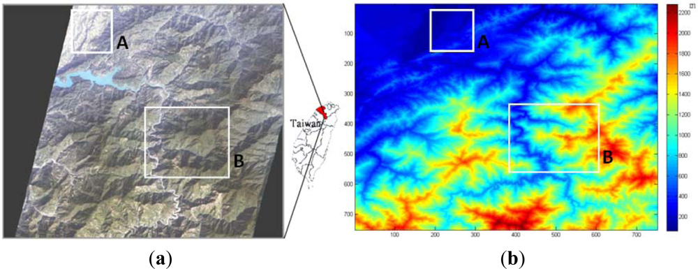
An area of approximately 750 km2 in northern Taiwan was chosen for this study (Figure 1). Terrain elevation in the area varies from 64 m to 2,284 m above the mean sea level. It encompasses different landcover types including forest, bare land, orchard plantations, suburban built-up, and water body (reservoir pools and rivers). The reservoir pool stretches roughly in the east-west direction near the northwestern corner of the study area. A major river and its tributaries flow from south to north across the center of the study area before entering the reservoir pool. Apart from a relatively small portion in the most northwestern corner in which a suburban township exists, most of the study area is dominated by forest landcover. There are also a few orchard plantations and bare land parcels scattered over the study area.
A set of Formosat-II multispectral images (including blue band: 450–520 nm, green band: 520–600 nm, red band: 630–690 nm, and near infrared band: 760–900 nm, with 8 m spatial resolution) of the study area acquired at 01:57 GMT (9:57 a.m. local time) on December 11, 2008 was collected (Figure 1(a)). The sun angle and view angles were 54.925° and 14.086° respectively, while azimuth angles of the satellite and the sun were 325.004° and 148.641°, respectively. DEM data of the study area (see Figure 1(b)) with a 40-m spatial resolution were also collected and used for topographic effect modeling. Elevation error of the 40-m DEM data has a mean of approximately 1 meter and standard deviation of 4 to 8 meters in mountainous region [21].
3. Methodology
3.1. At-Sensor Radiance Modeling
For a target of Lambertian surface, the at-sensor solar radiance of spectral wavelength λ, i.e., Lsλ, can be expressed by [10,16]
where
- (θ, ϕ)= the zenith and azimuth angles of the target-sun directions, respectively,
- Lpλ= path radiance,
- Eoλ= exoatmospheric solar irradiance with respect to spectral wavelength λ,
- Edλ= downwelled irradiance,
- rdλ= diffuse reflectance of the Lambertian surface,
- τ1λ= transmittance along the sun-target direction,
- τ2λ= transmittance along the target-sensor direction,
- F = shape factor due to obstruction of terrain slope or adjacent objects,
- σi= incidence angle of the solar irradiance at the target.
Radiances reaching the sensor are recorded and linearly converted to digital numbers (DNs) by the following equation using the band-specific gain and offset parameters of the sensor:
Thus, the equation of radiometric propagation (Equation (1)) can be rewritten as
where
The dependence of DNpλ, rdλ, k1λ, and k2λ on the wavelength λ, which can be considered as the central wavelength of a spectral band, indicates that these parameters are band-specific. For Formosat-II images used in this study, values of the offset parameter were zero for all spectral bands whereas values of the gain parameter were 0.3441, 0.3561, 0.2553 and 0.3062 (W·μm−1·m−2·sr−1) for the blue, green, red and near infrared bands, respectively. For local remote sensing applications which do not cover extensively wide study areas, the exoatmospheric solar irradiance, downwelled irradiance, path radiance, and atmospheric transmittances can all be assumed to be spatially homogeneous. In other words, DNpλ, k1λ and k2λ all can be viewed as constants for all ground samples. On the other hand, F and cosσi represent the topographic characteristics of individual ground samples and are the sources of topographic effects.
Cheng et al. [16] proposed a radiometric control areas (RCAs) approach for path radiance estimation. In their study, a radiometric control area is a horizontal and unobstructed area with spatially homogeneous and temporally stationary land surface condition. By considering only ground samples in radiometric control areas, the at-sensor radiance can be expressed as a linear regression function of surface reflectance with intercept being the path radiance. Thus, using in situ measurements of surface reflectance in the radiometric control areas, path radiance of the study area can be estimated by solving the linear equation. The idea of using ground samples in radiometric control areas is to eliminate the topographic effects in Equations (1) and (3). In this study we adopt a similar concept of radiometric control areas for estimation of surface reflectance.
3.2. Identification of Shaded Ground Samples
Although in general the at-sensor radiance can be expressed by Equation (1), there are situations in which solar irradiance cannot reach the target ground sample and should be dropped from Equation (1). As depicted in Figure 2(a), the target ground sample is located at the leeside of the solar irradiance (σi > 90°, cosσi < 0) and thus receives no incoming solar radiance. Whereas in Figure 2(b), incoming solar radiation is obstructed by surrounding objects and cannot be received at the target ground sample.
Under either situation, digital numbers of these ground samples (hereinafter referred to as the shaded ground samples) should be expressed by the following equation:
The shaded ground samples can be identified using DEM data and sun angle of the satellite image. A straightforward algorithm as demonstrated in Figure 3 was used in this study for calculation of cosσi of individual ground samples. From the DEM data, we first calculated the normal vector V⃗o of the target ground sample using the four normal vectors (U⃗i, i = 1, . . . , 4) determined by the target ground sample and its surrounding ground samples, i.e.,
The normal vector in the target-sun direction, i.e., V⃗s, is then determined by considering the latitude and longitude of the study area and the image acquisition time. Thus, cosσi can be easily obtained by
Similar to utilization of RCA samples by Cheng et al. [16], shaded ground samples eliminate the second term in the right-hand-side of Equation (3) and play a crucial role in this study.
3.3. Modeling of the Shape Factor F
The shape factor F in Equation (6) represents the proportion of the total downwelled radiance that can reach the target ground sample. If the downwelled radiance is homogeneous over the entire sky dome above the target sample, then the shape factor F represents the ratio of the solid angle subtended at the target ground sample by the downwelled-radiance-contributing sky dome to the solid angle of a hemisphere, i.e., 2π. Thus, it can be obtained by calculating the downwelled-radiance-receiving solid angle using DEM data. However, in reality the downwelled radiance may not be homogeneous at all time and thus the shape factor not only depends on the downwelled-radiance-receiving solid angle but also spatial variation of the downwelled radiance. Since spatial variation of the downwelled radiance is essentially random due to inhomogeneous distribution of atmospheric particles, the shape factor F can therefore be treated as a random variable. Thus, in this study we adopt a statistical approach for estimation of sample-specific shape factor F by taking into account the ground-sample-specific topographic characteristics.
For convenience of subsequent explanation, we first define the following notations which will be used later. Consider a group of p × p ground samples with the target ground sample located at the center. The size of this sample group (p × p) is carefully chosen such that its coverage is large enough to account for the solar radiation obstruction by surrounding objects, as illustrated in Figure 2(b). Let X be a vector consisting of the shape factor F associated to the target ground sample and elevation differences (Ei – E0 = di) between the target sample and its neighboring samples, i.e:
Vector partitions in the above equation are self-explaining with X1 = F and X2 represents and elevation differences (di, i=1, 2, ..., p2–1). Elevations of the target ground sample and its surrounding samples in the sample group are represented by an elevation matrix Elev which can be expressed by the following equation:
In this study the value of p was set to 41 so that all neighboring samples that may contribute to the shape factor are included in the 41 × 41 sample group. With a pixel size of 8-meter for Formosat-II multispectral images, a 41 × 41 sample group encompasses an area centered at the target sample and extending at least 160 meters outward in all directions.
Spatial variations of the shape factor X1 and elevation difference X2 within the study area can be considered as two random fields with their mean vectors and covariance matrices defined as
The shape factor F varies with locations and is considered as a random variable with a constant expectation μ1. For target samples with larger elevation differences between the target sample and its neighboring samples, i.e., X′2 = (d1, d2, ⋯, dp2–1), we can expect more significant obstruction effect and lower values of the shape factor. From the fundamental theorem of estimation theory [22], the best linear estimator (in terms of minimum mean-squared errors) of F, given the elevation differences X2 associated to the target ground sample, is the conditional expectation of F given by the following equation:
Substituting Equation (12) into Equation (13), it yields
Readers are reminded that x2 and μ2 in Equations (13) and (14) are vectors representing a realization and the expectation of X2, respectively.
The mean vector and covariance matrix (i.e., μ2 and Σ22) of X2 in Equation (14) can be obtained by calculating the sample mean and sample covariance of X2 using DEM data of a total of 388,000 ground samples within the study area. With the very large number of ground samples, estimates of μ2 and Σ22 can be expected to be nearly unbiased and with very small variance, even though X2 is likely to exhibit spatial dependence. As for Var(di) (i=1,...,p2–1) in Equation (14), they represent the diagonal elements of Σ22 and thus are readily available once Σ22 has been obtained.
Considering Lambertian targets and isotropic diffuse irradiance, surface reflectance of the target ground sample rdλ represents the inherent property of land surface and is independent of the shape factor F and the elevation differences of neighboring samples di (i=1,...,p2–1). Thus, if only shaded ground samples are considered, we have
Using the property of variance of product of independent random variables [23], we have
Thus,
In the above equations DNshade indicates digital numbers of shaded ground samples and Kλ is an unknown constant since it is completely determined by distribution parameters of F and rdλ. Thus, substituting Equation (16a) into Equation (14), it yields
Shaded ground samples account for approximately one sixth of the total number of ground samples in the study area. With this very large sample size and also based on the asymptotic distributional properties of the sample correlation coefficients [24],
(i=1,...,p2–1) can be estimated with near zero bias and very small variance. Thus, for every ground sample the sample-specific
value can be easily calculated using Equation (18). It is also worthy to note that although
and Kλ in Equation (17) are band-specific, the shape factor estimate F̂ is not band-dependent, as can be seen from Equation (14). The band-dependency will be eliminated by calculation of the product term
Kλ .
3.4. Estimation of Surface Reflectance Using RCA Samples
Suppose that a total of n ground samples from radiometric control areas with in situ measurements of surface reflectance are available. Digital numbers of these samples satisfy Equation (19) and can be expressed by the following matrix equation:
where superscript RCAi indicates attributes of RCA samples. For example,
represents the band-specific digital number of the i-th RCA sample.
In the above matrix equation, digital numbers and surface reflectances of RCA samples are known and cosσi and
can be calculated using Equation (8) and Equation (18), respectively. Thus, DNpλ, k1λ, k2λμ1 and k2λK can all be solved by the least-square multiple regression technique.
In previous sections we have demonstrated that values of DNpλ, k1λ, k2λμ1 and k2λKλ can be considered as constants for all ground samples for applications that do not cover extensively wide areas. Therefore, estimation of band-specific surface reflectances of non-RCA samples can be achieved by solving Equation (19) and Equation (20) for non-shaded and shaded ground samples, respectively.
4. Results and Discussion
4.1. Calculation of cosσi
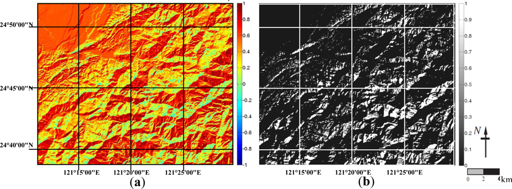
The topographic effect of cosσi calculated using Equation (8) is shown in Figure 4(a). In order to demonstrate the feasibility of using Equation (8) for modeling the topographic effect, we also rescaled grey levels of Formosat-II color image of the study area (see Figure 4(b)) and compared shaded areas in both figures. It can be observed that shaded areas in both images are largely consistent. Such results indicate the potential of characterizing the topographic effect by Equations (7) and (8), although more rigorous assessment, especially with respect to DEM accuracy, may be required.
4.2. Correlation Map of Shaded Ground Samples
As was explained in Section 3.3, the correlation coefficients between digital numbers of shaded ground samples (DNshade) and elevation differences of neighboring samples (di, i=1,...,p2–1) can be estimated with near zero bias and very small variance. These correlation coefficients
(i=1,...,p2–1) correspond to a group of p ×p (p=41) ground samples centered at the target sample, and can be arranged as the following correlation matrix P [24],
where
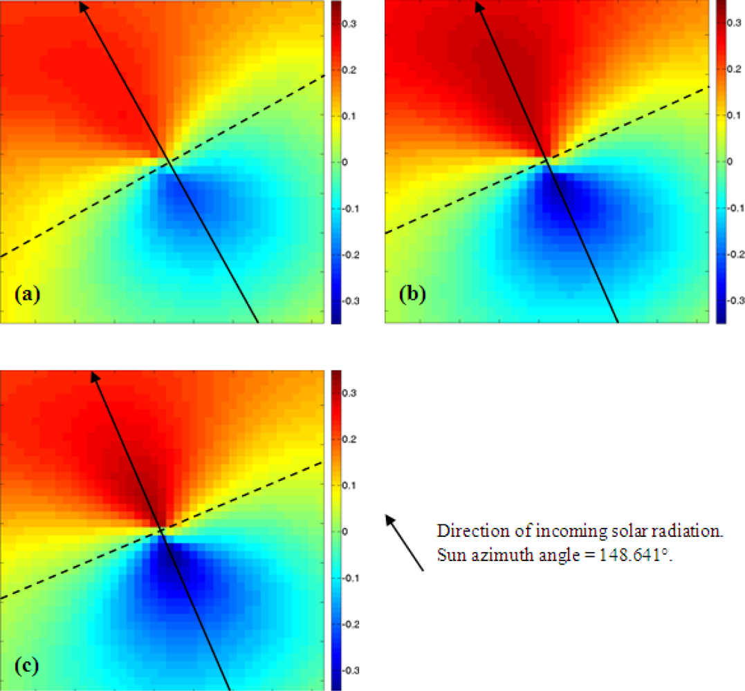
(i=0,...,p2–1). We shall refer to the correlation matrix Pλ as the correlation map since it characterizes the spatial pattern of the correlation between digital numbers of shaded samples and elevation differences of neighboring samples. Figure 5 demonstrates the estimated correlation maps of different spectral bands.
The correlation maps show a pattern nearly symmetric to the direction of incoming solar radiation for all spectral bands. Digital numbers (or corresponding radiances) of the shaded ground samples are contributed by the downwelled radiance from portion of the sky dome above the target sample. Downwelled radiances are the results of atmospheric scattering, most importantly the Rayleigh and Mie scatterings, whose effects are symmetric to the direction of solar irradiance. The symmetric pattern of the correlation map correctly reflects the characteristics of atmospheric scattering. The correlation map also shows that positive and negative correlation coefficients are associated with the samples falling in front of and in the back of the target sample (with respect to the target sample and the direction of solar irradiance), respectively. Such a pattern is also consistent with the topographic effects on radiance received at the target ground as explained below.
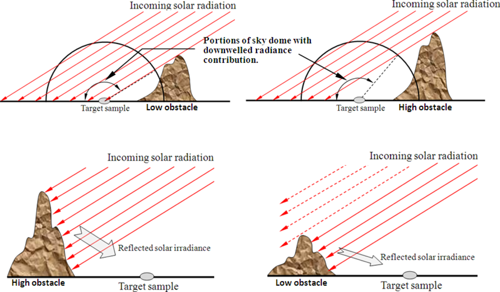
As shown in Figure 6, obstacle samples behind the target sample (with reference to the direction of incoming radiation) obstruct direct solar irradiance to the shaded target sample. The higher these obstacles (i.e., higher di values), the less downwelled radiance (smaller digital numbers) received at the target sample. Thus, for shaded ground samples DNshade and elevation differences of neighboring obstacle samples (di, i = 1,...,p2–1) are negatively correlated. In contrast, solar irradiances reaching the obstacle samples which situate in front of the target sample may be reflected to the target sample. The higher the obstacle samples (i.e., higher di values), the more reflected radiance (larger digital numbers) received at the target sample. Thus, DNshade and elevation differences of neighboring obstacle samples (di, i = 1,...,p2–1) are positively correlated.
Figure 5 also shows that correlation coefficients are lowest (at or near zero) for neighboring samples located in the direction perpendicular to the incoming solar radiation. This is explained by the fact that both the Rayleigh and Mie scattering effects are minimum in the direction perpendicular to the incoming solar radiation.
4.3. Assessing Estimates of Surface Reflectance
Prior to calculation of surface reflectances using Equations (19) and (20), band-dependent values of DNpλ, k1λ, k2λμ1 and k2λK must be calculated by solving Equation (21). In this study in situ reflectance measurements from a set of 150 RCA samples which scattered over the entire study area were collected using a multispectral radiometer. Band-dependent reflectances of these RCA samples were then used to calculate band-dependent constants DNpλ, k1λ, k2λμ1 and k2λK (see Table 1) by solving Equation (21).
Among these constants, values of DNpλ represent the band-specific path radiances which in principle decrease with increasing wavelength λ of solar radiation since the effect of atmospheric scattering (mainly including the Rayleigh scattering and the Mie scattering) reduces with increasing wavelength of solar radiation. Table 1 shows that band-dependent DNpλ values estimated by the method proposed in this study are consistent with effect of atmospheric scattering. Cheng et al. [15] used the same set of Formosat II images for path radiance estimation using the dark object subtraction (DOS) method and AERONET measurements of molecule and aerosol optical depths (AODs) (see Table 2). The DOS method tends to overestimate the path radiance if the selected dark objects are not near-zero reflectors, especially in mountainous areas [10,15]. The proposed method seems to yield more reasonable results than the commonly used DOS method with their path radiance estimates closer to path radiances calculated using AERONET measurements.
Since the study area encompasses an area of 750 km2 with different land cover conditions, it is difficult to conduct extensive in situ measurements of surface reflectance and validate estimates of surface reflectance by the proposed method. Thus, in this study we selected two subregions which represent moderate and high degree of terrain variation in our study area and visually compared their corresponding true color satellite images and color reflectance images. As demonstrated in Figure 7, color reflectance image (using blue, green and red colors for reflectances of the blue, green and red bands) and the true color satellite image of the subregion A (moderate terrain variation with elevation varies from 0 to approximately 600 m above the mean sea level) are very similar, indicating good estimates of surface reflectance in this region. Differences in reflectances of the water body, vegetation, built-up, and bared soils are well preserved in the color reflectance image. It can also be observed that shaded areas are present in the east and southeast corner of the true color satellite image of subregion A, whereas such shade effect has largely diminished in the color reflectance image since surface reflectances only depend on landcover types and are not affected by the topographic condition.
True color satellite image of the subregion B which is an area with high mountains and substantial terrain variation (elevation varies from approximately 200 to 2000 m) shows significant topographic effect with visually apparent shaded areas. Although the topographic effect has also been largely eliminated in the color reflectance image of subregion B, the reflectance image still shows different levels of reflectance for the shaded (in purple color) and non-shaded (in green color) areas. Such results may arise from the unaccounted shade effect of very high mountains in subregion B. In our study an elevation matrix (Equation (10)) of 41×41 sample group is adopted and calculation of the shape factor considers only neighboring samples within the 160-m range of the target sample. High mountains not within the 160-m range may also block solar irradiance and cast shade on the target sample and such effect has not been considered in our analysis. It also indicates that elevation matrices of larger size may need to be used for areas of more significant terrain variation. Further study on determining the size of the elevation matrix and the correlation map with respect to the degree of elevation change (or terrain variation), i.e., variable size of elevation matrix, may help to improve reflectance estimation in areas with substantial terrain variation. It is also important to mention that the proposed method requires in situ reflectance measurements and DEM data. Thus, for areas without DEM data or for historical remote sensing data with no in situ reflectance values, application of the proposed method cannot be implemented.
5. Conclusions
This study is an extension of the RCA-based path radiance estimation algorithm for surface reflectance estimation using digital numbers and surface reflectance of selected radiometric control areas. A few concluding remarks are drawn as follows:
- A shaded sample identification algorithm using DEM data is proposed in this study.
- The correlation maps demonstrate a pattern that not only is consistent with the atmospheric scattering effect but also characterizes the effect of neighboring samples on radiance received at the target sample. Such result is an indication that the proposed shape factor model (Equation (14)) is physically reasonable.
- The proposed RCA-based surface reflectance estimation method is capable of achieving good reflectance estimates in a region where elevation varies from 0 to approximately 600 m above the mean sea level. Further study on variable size of the elevation matrix with respect to the degree of terrain variation is recommended in order to extend application of the proposed method to areas with substantial terrain variation.
Acknowledgments
The corresponding author is grateful to the National Science Council (NSC) of Taiwan, ROC for its financial support of his sabbatical leave during which this manuscript was completed. The corresponding author would like to dedicate this paper to the Late Professor Toshiharu Kojiri of the Disaster Prevention Research Institute, Kyoto University, who hosted the sabbatical visit of the corresponding author and had many fruitful and interesting discussions with him. We are also grateful to two anonymous reviewers for their constructive comments which led to a much better presentation of the final form of this paper.
References
- Weismiller, R.A.; Kristof, S.J.; Scholtz, D.K.; Anuta, P.E.; Momin, S.A. Change detection in coastal zone environments. Photogramm. Eng. Remote Sensing 1977, 43, 1533–1539. [Google Scholar]
- Vogelmann, J.E. Detection of forest change in the Green Mountains of Vermont using multispectral scanner data. Int. J. Remote Sens 1988, 9, 1187–1200. [Google Scholar]
- Nielsen, A.A.; Conradsen, K.; Simpson, J.J. Multivariate alteration detection (MAD) and MAF postprocessing in multispectral, bitemporal image data: new approaches to change detection studies. Remote Sens. Environ 1998, 64, 1–19. [Google Scholar]
- Teng, S.P.; Chen, Y.K.; Cheng, K.S.; Lo, H.C. Hypothesis-test-based landcover change detection using multi-temporal satellite images. Adv. Space Res 2008, 41, 1744–1754. [Google Scholar]
- Gates, D.M.; Keegan, H.J.; Schleter, J.C.; Weidner, V.R. Spectral qualities of plants. Appl. Opt 1965, 4, 11–20. [Google Scholar]
- Tucker, C.J. Red and photographic infrared linear combinations for monitoring vegetation. Remote Sens. Environ 1979, 8, 127–150. [Google Scholar]
- Tucker, C.J.; Holben, B.N.; Elgin, J.H.; Mcmurtrey, J.E. Relation of spectral data to grain yield variation. Photogramm. Eng. Remote Sensing 1980, 46, 657–666. [Google Scholar]
- Asrar, G.; Fuchs, M.; Kanemasu, E.T.; Hatfield, J.L. Estimating absorbed photosynthetic radiation and leaf area index from spectral reflectance in wheat. Agron. J 1984, 76, 300–306. [Google Scholar]
- Slater, P.N. Remote Sensing: Optics and Optical Systems; Addison-Wesley: Reading, MA, USA, 1980; p. 592. [Google Scholar]
- Schott, J.R. Remote Sensing: The Image Chain Approach, 2nd ed.; Oxford University Press: New York, NY, USA, 2007; p. 688. [Google Scholar]
- Liang, S.; Fang, H.; Chen, M. Atmospheric correction of Landsat ETM+ land surface imagery: Part I: Methods. IEEE Trans. Geosci. Remote Sens 2001, 39, 2490–2498. [Google Scholar]
- Forster, B.C. Derivation of atmospheric correction procedures for Landsat MSS with particular reference to unban. Int. J. Remote Sens 1984, 5, 799–817. [Google Scholar]
- Chavez, P.S., Jr. An improved dark-object subtraction technique for atmospheric scattering correction of multispectral data. Remote Sens. Environ 1988, 24, 459–479. [Google Scholar]
- Chavez, P.S., Jr. Radiometric calibration of Landsat Thematic Mapper multispectral images. Photogramm. Eng. Remote Sensing 1989, 55, 1285–1294. [Google Scholar]
- Moran, M.S.; Jackson, P.N.; Slater, P.N.; Teillet, P.M. Evaluation of simplified procedures for retrieval of land surface reflectance factors from satellite sensor output. Remote Sens. Environ 1992, 41, 169–184. [Google Scholar]
- Cheng, K.S.; Su, Y.F.; Yeh, H.C.; Chang, J.H.; Hung, W.C. A path radiance estimation algorithm using reflectance measurements in radiometric control areas. Int. J. Remote Sens 2012, 33, 1543–1566. [Google Scholar]
- Switzer, P.; Kowalik, W.; Lyon, R.J.P. Estimation of atmospheric path-radiance by the covariance matrix method. Photogramm. Eng. Remote Sensing 1981, 47, 1469–1476. [Google Scholar]
- Mueller, R.; Behrendt, T.; Hammer, A.; Kemper, A. A new algorithm for the satellite-based retrieval of solar surface irradiance in spectral bands. Remote Sens 2012, 4, 622–647. [Google Scholar]
- Viggh, H.E.M.; Staelin, D.H. Spatial surface prior information reflectance estimation (SPIRE) algorithms. IEEE Trans. Geosci. Remote Sens 2003, 41, 2424–2435. [Google Scholar]
- Wen, J.; Liu, Q.; Liu, Q.; Xiao, Q.; Li, X. Parametrized BRDF for atmospheric and topographic correction and albedo estimation in Jiangxi rugged terrain, China. Int. J. Remote Sens 2009, 30, 2875–2896. [Google Scholar]
- Yang, S.Z.; Tseng, Y.H. Quality assessment for Digital Elevation Models. Journal of Photogrammetry and Remote Sensing 2008, 13, 195–206, (In Chinese with English abstract). [Google Scholar]
- Mendel, J.M. Lessons in Estimation Theory for Signal Processing, Communications, and Control; Prentice Hall: Upper Saddle River, NJ, USA, 1995; p. 561. [Google Scholar]
- Goodman, L.A. On the exact variance of products. J. Am. Statist. Assoc 1960, 55, 708–713. [Google Scholar]
- Neudecker, H.; Wesselman, A.M. The asymptotic variance matrix of the sample correlation matrix. Linear Algebra Its Appl 1990, 127, 339–599. [Google Scholar]
Figure 1.
(a) Formosat-II image of the study area. (b) Digital elevation model (DEM image of the study area. Two subregions A and B (also seen in figure in Section 4.3) of different degrees of terrain variation were selected for assessment of reflectance estimation by the proposed approach.
Figure 1.
(a) Formosat-II image of the study area. (b) Digital elevation model (DEM image of the study area. Two subregions A and B (also seen in figure in Section 4.3) of different degrees of terrain variation were selected for assessment of reflectance estimation by the proposed approach.

Figure 2.
Sun/shade occurrences: (a) Irradiance not reaching the target object; (b) Solar irradiance blocked by surrounding obstacles.
Figure 2.
Sun/shade occurrences: (a) Irradiance not reaching the target object; (b) Solar irradiance blocked by surrounding obstacles.

Figure 3.
An illustrative sketch for calculation of cosσi.

Figure 4.
Images showing topographic effects. (a) cosσi image. (b) Transformed grey level of Formosat-II color image. Numbers of scale bars represent values of cosσi and transformed grey level (between 0 and 1). Negative values of cosσi and extremely high values of grey level represent shaded ground samples.

Figure 5.
Correlation map Pλ calculated from satellite images of different spectral bands. (a) Blue. (b) Green. (c) Red. Numbers of the scale bar represent values of the correlation coefficient.
Figure 5.
Correlation map Pλ calculated from satellite images of different spectral bands. (a) Blue. (b) Green. (c) Red. Numbers of the scale bar represent values of the correlation coefficient.

Figure 6.
Illustration of the topographic effects of the forward and backward samples on radiance (or digital number) received at the target sample.
Figure 6.
Illustration of the topographic effects of the forward and backward samples on radiance (or digital number) received at the target sample.

Figure 7.
Comparison of the true color satellite images (left) and the color reflectance images (right) of the study area and its two subregions.
Figure 7.
Comparison of the true color satellite images (left) and the color reflectance images (right) of the study area and its two subregions.


Table 1.
Band-dependent constants (DNpλ, k1λ, k2λμ1 and k2λK) for calculation of surface reflectance.
| Blue Band | Green Band | Red Band | |
|---|---|---|---|
| DNpλ | 59 | 19 | 8 |
| k1λ | 346.011 | 358.119 | 279.024 |
| k2λμ1 | 269.372 | 333.391 | 544.729 |
| k2λK | 47.662 | 36.112 | 28.326 |
| Methods | Blue Band | Green Band | Red Band |
|---|---|---|---|
| This study | 59 | 19 | 8 |
| DOS | 69 | 36 | 26 |
| AERONET | 29 | 19 | 13 |
Note: Path radiances of the DOS and AERONET methods were estimated by Cheng et al. [16].
Share and Cite
MDPI and ACS Style
Chen, H.-W.; Cheng, K.-S. A Conceptual Model of Surface Reflectance Estimation for Satellite Remote Sensing Images Using in situ Reference Data. Remote Sens. 2012, 4, 934-949. https://doi.org/10.3390/rs4040934
AMA Style
Chen H-W, Cheng K-S. A Conceptual Model of Surface Reflectance Estimation for Satellite Remote Sensing Images Using in situ Reference Data. Remote Sensing. 2012; 4(4):934-949. https://doi.org/10.3390/rs4040934
Chicago/Turabian StyleChen, Hsien-Wei, and Ke-Sheng Cheng. 2012. "A Conceptual Model of Surface Reflectance Estimation for Satellite Remote Sensing Images Using in situ Reference Data" Remote Sensing 4, no. 4: 934-949. https://doi.org/10.3390/rs4040934