Next Article in Journal
A Semi-Automated Object-Based Approach for Landslide Detection Validated by Persistent Scatterer Interferometry Measures and Landslide Inventories
Previous Article in Journal
Biome-Scale Forest Properties in Amazonia Based on Field and Satellite Observations
 
 
remotesensing-logo
Article Menu

Article Menu

Review

Review of the CALIMAS Team Contributions to European Space Agency’s Soil Moisture and Ocean Salinity Mission Calibration and Validation

by
Adriano Camps
1,2,*,
Jordi Font
2,3,
Ignasi Corbella
1,2,
Mercedes Vall-Llossera
1,2,
Marcos Portabella
2,4,
Joaquim Ballabrera-Poy
2,4,
Verónica González
2,3,
María Piles
1,2,
Albert Aguasca
1,
René Acevo
1,
Xavier Bosch
5,
Nuria Duffo
1,2,
Pedro Fernández
2,3,
Carolina Gabarró
2,3,
Jérôme Gourrion
2,3,
Sébastien Guimbard
2,3,
Anna Marín
6,
Justino Martínez
2,3,
Alessandra Monerris
7,
Baptiste Mourre
8,
Fernando Pérez
2,3,
Nereida Rodríguez
1,2,
Joaquín Salvador
2,3,
Roberto Sabia
9,
Marco Talone
10,
Francesc Torres
1,2,
Miriam Pablos
1,
Antonio Turiel
2,4,
Enric Valencia
1,2,
José Martínez-Fernández
11,
Nilda Sánchez
11,
Carlos Pérez-Gutiérrez
11,
Guido Baroncini-Turricchia
11,
Antonio Rius
12 and
Serni Ribó
12
add Show full author list remove Hide full author list
1
Dept. Teoria del Senyal i Comunicacions, Universitat Politècnica de Catalunya and IEEC/UPC, c/Jordi Girona 1-3, Campus Nord, E-08034 Barcelona, Spain
2
SMOS Barcelona Expert Centre, CSIC-UPC, Pg. Marítim Barceloneta, 37-49, E-08003 Barcelona, Spain
3
Institut de Ciències del Mar (ICM-CSIC), Pg. Marítim Barceloneta 37-49, E-08003 Barcelona, Spain
4
Unitat de Tecnologia Marina (UTM-CSIC), Pg. Marítim Barceloneta 37-49, E-08003 Barcelona, Spain
5
Electrical & Computer Engineering, Colorado State University, 1373 Campus Delivery, Fort Collins, CO 80523, USA
6
Centre de Recerca Ecològica i d’Aplicacions Forestals, Edifici C, Campus de la UAB, E-08193Bellaterra, Spain
7
Department of Civil Engineering, Room 147, Building 60, Clayton Campus, Monash University, Clayton, VIC 3800, Australia
8
NURC, Viale San Bartolomeo 400, I-19126 La Spezia, Italy
9
ESA/ESRIN, Via Galileo Galilei, Casella Postale 64, Frascati, I-00044 Rome, Italy
10
Serco SpA, Via Sciadonna, 24/26 Frascati, I-00044 Rome, Italy
11
Centro Hispano Luso de Investigaciones Agrarias (CIALE), University of Salamanca, E-37185 Villamayor, Spain
12
IEEC/ICE-CSIC, Universitat Autònoma de Barcelona, C5/242, E-08193 Bellaterra, Spain
*
Author to whom correspondence should be addressed.
Remote Sens. 2012, 4(5), 1272-1309; https://doi.org/10.3390/rs4051272
Submission received: 13 March 2012 / Revised: 17 April 2012 / Accepted: 18 April 2012 / Published: 4 May 2012

Abstract

:
This work summarizes the activities carried out by the SMOS (Soil Moisture and Ocean Salinity) Barcelona Expert Center (SMOS-BEC) team in conjunction with the CIALE/Universidad de Salamanca team, within the framework of the European Space Agency (ESA) CALIMAS project in preparation for the SMOS mission and during its first year of operation. Under these activities several studies were performed, ranging from Level 1 (calibration and image reconstruction) to Level 4 (land pixel disaggregation techniques, by means of data fusion with higher resolution data from optical/infrared sensors). Validation of SMOS salinity products by means of surface drifters developed ad-hoc, and soil moisture products over the REMEDHUS site (Zamora, Spain) are also presented. Results of other preparatory activities carried out to improve the performance of eventual SMOS follow-on missions are presented, including GNSS-R to infer the sea state correction needed for improved ocean salinity retrievals and land surface parameters. Results from CALIMAS show a satisfactory performance of the MIRAS instrument, the accuracy and efficiency of the algorithms implemented in the ground data processors, and explore the limits of spatial resolution of soil moisture products using data fusion, as well as the feasibility of GNSS-R techniques for sea state determination and soil moisture monitoring.

1. Introduction

On 2 November 2009 the European Space Agency successfully launched from Plesetsk, (Northern Russia) the first of its Earth Explorer Opportunity Missions: SMOS, which stands for Soil Moisture and Ocean Salinity [14]. These are small format missions aimed at demonstrating new technologies to provide relevant new information for Earth observation from space, which are submitted to ESA by the scientific community through dedicated calls. SMOS was proposed in 1998 and the scientific objectives are two-fold: to generate global soil moisture (SM) and sea surface salinity (SSS) maps. Both variables are fundamental to understand the evolution of the water cycle on Earth and its impact on climate. Taking into account the expected technical constraints and the range of environmental issues SMOS could address, the mission requirements were definitively established in 2002 so as to deliver SM estimates with an accuracy better than 0.04 m3/m3 at a spatial resolution better than 50 km every three days minimum over continental surfaces, and SSS estimates with an accuracy of the order of 0.1 psu, every 10 (30) days in boxes of 200 (100) km over the oceans.
SMOS is based on an innovative technical concept, never used before in Earth observation: microwave interferometric radiometry. SMOS’ single payload is MIRAS, the Microwave Imaging Radiometer with Aperture Synthesis, developed by EADS-CASA Espacio (Spain) for ESA [5]. Every 1.2 s MIRAS reconstructs a snapshot brightness temperature (TB) image of a large field-of-view from the power recorded by 69 small antennas spread over a Y-array with three ∼4-m long arms. This provides a wide range of incidence angles for the observation of any point on the Earth’s surface in a single orbit, one of the major characteristics of SMOS is to retrieve SSS and SM from the radiometric measurements (see e.g., [6]).
Both geophysical variables have a common feature: they modify the dielectric properties of seawater and soil, respectively. MIRAS, operating at 1.413 GHz, captures information on the spatial and temporal variability of the dielectric constant, from which retrievals of SM and SSS are made [7,8]. However, due to the low sensitivity of TB to SSS [9] even at this almost optimal frequency, the range of TB that corresponds to the entire range of salinity values in the world oceans (about 5 K at a fixed incidence angle [10]) is 20 times smaller than the corresponding range for soil moisture. This means that retrievals over land, even affected by a large variety of soil types and topographic effects that make difficult the emission modeling [11], are more robust than retrievals over ocean. As such, requirements for the instrument performance in terms of sensitivity, calibration, and stability are less strict for SM than for SSS (see e.g., [4,12]). The retrieval of SSS by SMOS is a challenging task that has required (and still requires) an important effort from all the teams involved in MIRAS calibration, image reconstruction techniques, ocean forward modeling, quality control, and SSS retrievals. This effort has allowed the acquirement of the first ever satellite measurements of sea surface salinity [13] with a quality that is progressively approaching the mission requirements through successive improvements introduced in the data processing ([14]).
This work summarizes the recent contributions from the CALIMAS (“CALibration-validation of Interferometric Microwave And Salinity products”) project aimed at SMOS calibration and validation. The objectives of this project, submitted in 2005 to the ESA Announcement of Opportunity for SMOS Cal/Val, are:
  • The assessment of SMOS calibration, stability and image reconstruction algorithms;
  • The preliminary assessment of salinity retrieval algorithms and validation of SMOS salinity products;
  • The assessment of sea surface salinity errors sources in a regional simulation of a numerical model;
  • The verification of SMOS image reconstruction and ocean salinity (and soil moisture) retrieval with the small airborne MIRAS; and
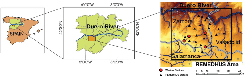
  • The assessment of mixed pixel effects and disaggregation techniques in the REMEDHUS soil moisture network (Zamora, Spain).
The contributions reported here will therefore span over these different topics, which all share a common objective: to improve the instrument calibration strategy and the data processing algorithms for the successful accomplishment of the mission objectives.
As previously explained, an outstanding instrument performance and an accurate image reconstruction are required for a successful SSS retrieval. As such, these processing steps (level 1 and level 2 salinity) have been addressed in a linked way. The questions analyzed at low level (Section 2 of this manuscript) include the characterization of the on-board stability and sensitivity of the power measurement systems (PMS), and how to compensate for the drifts detected in the data through an appropriate calibration strategy. A dedicated “MIRAS Testing Software”, independent of the official ground-processors, has been used for this purpose and to evaluate the quality of the TB obtained after the image reconstruction. Is the system performing as theoretically predicted? One of the most serious problems faced by SMOS at level 1 (L1) is the impact of radio frequency interference (RFI) in the protected band used by MIRAS. What algorithms can be proposed to efficiently detect and cancel the corrupted measurements?
In the domain of salinity retrieval (Section 3) the basic questions to be answered are related to the quality of the SMOS L1 products. Do the levels of bias and noise of the TB images allow a SSS retrieval within specifications? Are additional corrections required to compensate for residual imperfections after an optimal instrument calibration? In Section 3 we introduce the first salinity retrievals from airborne MIRAS demonstrators previous to SMOS launch, which helped to identify some of the problems that would later appear in the actual SMOS measurements (Section 3.1). In Section 3.2 we address the problem of removing a residual bias present in the reconstructed image, mainly due to uncorrected instrument imperfections and to the impact of the land-ocean transitions. After performing the bias corrections, it is important to assess the quality of the SSS retrievals and to analyze the possible causes for the achieved performance. Section 3.3 contains the CALIMAS team preliminary contribution to validate the SMOS SSS retrievals with in situ information, and in Section 3.4 we assess the sources of error in SSS products with a numerical model as part of preparatory studies for SMOS ocean data assimilation.
The second part of this work goes beyond the calibration and validation of the SMOS data, and focuses on the development of added-value level 4 (L4) products and the potential for further advancements. How could the mission deliverables be improved by means of additional information? In Section 4, the results of a downscaling technique developed to increase the SMOS resolution over land down to 1 km by combining SMOS and MODIS data are presented and discussed. As a prospect for future improvements in an eventual SMOS follow-on mission, Section 5 presents an assessment of the use of GNSS-R techniques (Global Navigation Satellite Systems signals-Reflectometry) to complement SMOS data and therefore improve the retrievals both over land and over ocean.
Finally, Section 6 presents a summary of the CALIMAS results and draws some conclusions in the context of their contribution to the current SMOS data processing state-of-the-art.

2. Results and Discussion

The main issues related to the MIRAS instrument concern its accurate calibration, the assessment and improvement of the image reconstruction algorithms, and the detection of radio-frequency interferences, and—eventually—their mitigation. The following sections summarize the main contributions.

2.1. Instrument Calibration

Calibration of such a complex instrument as MIRAS is fundamental to accurately retrieve soil moisture and ocean salinity. The MIRAS Testing Software (MTS) was developed by the UPC to process SMOS raw data from level 0 to level 1c and obtain geo-located brightness temperatures [15], applying the calibration procedures detailed in [16], and a number of image reconstruction algorithms. MTS has been extensively used during the on-ground characterization of the instrument to assess the MIRAS instrument performance. Besides, it has also been used to assess the operation of the payload during the first months after launch and to cross-validate and consolidate the products up to level 1A provided by the official L1 Processor Prototype (L1PP) developed by Deimos Enginheria (Portugal) [17].
As part of the commissioning phase tests, MTS has been used to assess the thermal and electrical stability and compare the results with those obtained during the on-ground characterization [18]. Among a number of different studies, a few important ones are explained below:
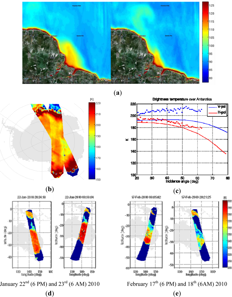
  • The analysis of the PMS offset jumps was found to be linked to the signal controlling the heaters (Figure 1(a)). A correction was implemented to estimate the offset from its mean value, the physical temperature, and the heater signals. After this correction, the residual offsets presented only the random fluctuation due to thermal noise and small physical temperature drift (Figure 1(b)).
  • The re-analysis of the PMS gain sensitivity to the in-orbit physical temperature drifts. These sensitivity values have been used to properly calibrate these gains (Figure 1(c), red line). The obtained calibrated values are consistent with the ones obtained during the on-ground characterization (Figure 1(c), blue line).
  • The analysis of the local oscillator (LO) phase drifts impact on the phase of the complex correlators’ gain for baselines not sharing a common LO. It was found that these baselines present a significant variation, which was not related to the physical temperature drifts of the receivers involved, but to the LO phase drift [19]. In-orbit local oscillator phase drifts have also been analyzed to determine the optimum inter-calibration period. Figure 1d shows the phase evolution of a given baseline when the LO calibration rate is 6 minutes and the phase is interpolated between calibrations considering an inter-calibration period of 12 min. The optimal LO calibration frequency is still under investigation, and some studies suggest that the optimum period is around 6–7 min [20]. After a proper characterization of the calibration system (CAS) with deep sky observations and cross-check with on-ground measurements, MIRAS calibration using internal and external modes was performed [21,22].

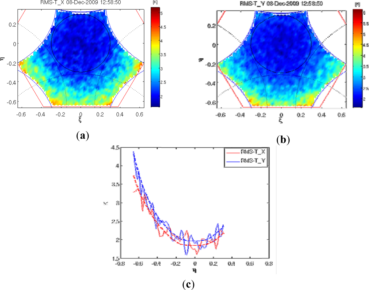
2.2. Image Reconstruction

MTS also implements a number of image reconstruction techniques, either assuming an ideal case, based on hexagonal FFTs [23] followed by an average antenna pattern compensation, or based on the characterized instrument and using G-matrix [2426]. This has enabled the evaluation of the quality of the brightness temperatures retrieved in the alias-free field of view (AF-FOV) including the radiometric resolution and the systematic spatial errors. Figure 2(a,b) shows the radiometric sensitivity estimated from Pacific Ocean images, free from coastal effects, at horizontal (Figure 2(a)) and vertical (Figure 2(b)) polarizations. Figure 2(c) represents a cut at ξ = 0 and the comparison between the measured values and the theoretical ones [27,28], with a very good agreement between the measurements and the theoretical predictions.
Brightness temperature images over the ocean, ice and land have been also produced using MTS. All the images presented below correspond to half the first Stokes parameter ((TV + TH)/2) in the alias-free field-of-view (AF-FOV). Figure 3 presents first checks of the general validity of SMOS images. Figure 3(a) shows the brightness temperature at the Amazon River, the plume being noticeable and the increase of the brightness temperature due to the entry of fresh water into the Atlantic Ocean. Brightness temperature images over ice, in particular over the Concordia Station (Dome-C area) in Antarctica are shown in Figure 3(b) and compared with the published data of DOMEX 2004 campaign (Figure 3(c)) [29]. Note that the biases at both polarizations are different, which is due to different calibration errors, since neither the Flat Target Transformation, nor the Ocean Target Transformation is applied. Regarding land applications, brightness temperature images have been retrieved over Australia before (Figure 3(d)) and after (Figure 3(e)) the Olga tropical storm both for ascending and descending orbits. Images show a strong decrease in the brightness temperatures, which is correlated to the increase of the soil moisture after the strong rain event. These results are in agreement with the rainfall anomalies measured over Australia by the TRMM mission from 17 January to 16 February 2010 (Figure 3(f) from [30]). Quality brightness temperature maps have been retrieved in the AF-FOV over land, ocean and ice using the MTS, showing structures compatible with soil moisture over land and salinity over ocean.

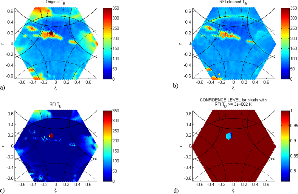
2.3. Radio Frequency Interference Detection and Mitigation

Despite the fact that preparatory field experiments had already demonstrated the RFI problem [31,32], when SMOS was turned on, the extension and intensity of RFI appeared so evident, that it became one of the most important problems to tackle. RFI extends over large areas of the world, mainly in Europe, Middle East and Asia, due to the different frequency allocations [33]. Since RFI is highly variable in time and polarization, average values of previous information cannot be reliably used. In addition, the number of RFI sources is highly variable and they can be (and most of them actually are) outside the AF-FOV (aliased regions of the image), but their impact (tails of the “impulse response”) is still present in the alias-free field of view. Therefore, the algorithms developed for SMOS RFI detection/mitigation operate on a snapshot basis only, and over the whole TB image (complete hexagonal period).
Two RFI detection/cancellation algorithms have been developed by the team. The first one [34] was developed during the first half of 2010, and it was conceived to operate on dual-polarization data only. Actually, it was an extension of the Sun cancellation algorithm in SMOS imagery [35,36], but applied recursively for all the RFI sources found. However, as compared to the Sun cancellation algorithm, a number of difficulties appeared: (a) as opposed to the Sun, the exact locations of the RFI sources are not known, so the position estimation has a limited accuracy given by the (ξ,η) director cosines grid size; (b) since the equivalent brightness temperature of the RFI (power received at the antenna divided by the Boltzmann constant and the radiometer’s bandwidth) is usually much lower that the brightness temperature of the Sun, the estimation of the background average temperature becomes more critical, and since most RFI sources are in coastal regions (land/sea), where the world’s population is concentrated, the estimation of the background average temperature is even more difficult. At the end of the commissioning phase it was decided that MIRAS will operate in full-polarimetric mode only. Then, even though in principle the above algorithm could be applied in dual from full-polarimetric data, an added difficulty was found. MIRAS is not really a full-polarimetric instrument, but it encompasses the full Stokes vector after the image reconstruction, and after a polarization switching sequence detailed in [37]. Since RFI is usually pulsed, then it is not usually present in all the switching steps, and the shape of the impulse response to that particular RFI is no longer the instrument’s impulse response, but varies depending on when the RFI occurred during the acquisition sequence.
This led to the development of a new detection/cancellation algorithm based on RFI detection by analysis of the four Stokes images individually, flagging the pixels suspect of RFI contamination in any of them, followed by object removal and exemplar-based region filling algorithms to interpolate the missing data. More details on the algorithm implementation can be found in [38]. Figure 4 shows the results of the proposed RFI detection/cancellation algorithm over real SMOS data acquired over the Caribbean sea: (a) the original brightness temperature image corrupted by a strong RFI, (b) the RFI “cleaned” brightness temperature; (c) the estimated RFI, and (d) the confidence of the RFI sources removed level (from 0 to 1, 0 being totally unreliable, and 1 being totally reliable). Typically, the larger the RFI-contaminated area that is removed, the lower the confidence level is towards the center of the source.

3. Preliminary Assessment of Ocean Salinity Retrieval Algorithms

The main issues related to the sea surface salinity retrievals from SMOS are discussed in depth in [2] and [39]. Font et al. [13] provided a first analysis of SMOS data one year after launch in terms of practical problems encountered in salinity retrieval. The weak sensitivity of the brightness temperatures vs. salinity hinders the salinity retrieval, and averaging is required over 10 to 30 days to reduce random errors. However, SMOS brightness temperatures suffer from biases that limit the effectiveness of the averaging procedure, and at the same time, the TB dependence on the sea state is not fully understood. In this section, the first sea surface salinity retrievals using two-dimensional interferometric radiometers are presented, followed by the main results of different bias cancellation strategies, the so-called Ocean Target Transformation (OTT), the validation of SMOS salinities with experimental surface salinity measurements obtained in a field experiment, and finally an assessment of SSS error sources in a numerical model regional simulation.

3.1. Early Sea Surface Salinity Retrievals Using Two-Dimensional L-band Interferometric Radiometers

Early salinity retrieval tests with the airborne MIRAS (AMIRAS or SMOSillo, little SMOS) were carried out over lake Lohja (Finland, June–July 2006) using just TX and TY (the antenna temperatures in the X and Y axes in the antenna reference frame) along ξ = 0, for which TX ≡ TH (TB at horizontal polarization) and TY ≡ TV (TB at vertical polarization). Due to the way SMOSillo was mounted in the Short SC-7 Skyvan aircraft of the Laboratory of Space Technology of the Helsinki University of Technology (HUT, now Aalto University), the range of incidence angles spanned only from 5° to 35°. After correcting for the sky and atmospheric downwelling contributions scattered in the sea, the SSS was retrieved from a least squares minimization of the measured and the modeled TBs (3-parameter retrieval: salinity, temperature, and effective wind speed) without using restrictions in the auxiliary parameters, except for a hard limit from 0 to 38 psu for SSS, from 0 to 20 m/s in the wind speed (WS), and from 0 to 20 °C for Sea Surface Temperature (SST) [40]. Results of the minimization in terms of the first Stokes parameter (I = TH + TV = TX + TY), which partially compensated the instrumental systematic errors between X- and Y-polarizations, without restrictions on the SST and WS led to retrieved salinity values between 0.30 and 0.53 psu depending on the initial guess (0 or 38 psu, respectively), both in good agreement with the expected salinity (fresh water). The retrieved SST (4.2 °C) and the effective WS (8.4 m/s) values (3-parameter retrieval) presented a larger error, but were not too far apart from the measurements reported by the Lohja Weather Station for that date: 8 °C surface temperature and average 0.6 m/s wind speed with 6.3 m/s peaks.
Due to a technical problem with some receivers, SMOSillo was no longer available, and in subsequent studies we used COSMOS-OS data acquired with the HUT-2D (HUT airborne U-shaped 2D L-band radiometer, [41]) mounted on the Skyvan, on August 13th and 15th, 2007 using the HUT-2D. Additionally, a vessel navigating at the same time along the aircraft ground-track measured sea surface temperature with a manual digital thermometer and surface water samples were collected every 150 m, to be analyzed later by the Finnish Marine Research Institute.
Figure 5(a) shows the campaign area, together with the locations of the salinity measurements carried out by the vessel (stars) and interpolated to the SSS retrieval grid. Figure 5(b) shows the salinity retrievals without bias compensation, with a constant bias, and with external brightness temperature calibration, and Figure 5(c) shows the salinity retrievals in 2° bins, using the external brightness temperature calibration [42] and the salinity calibration [43], and after performing the spatial averaging. The results of this study [44] showed a better performance of the first Stokes parameter over the use of TX and TY, and anticipated the clear need to perform a calibration of the BT biases that appear in the image reconstruction process, prior to the salinity retrievals.

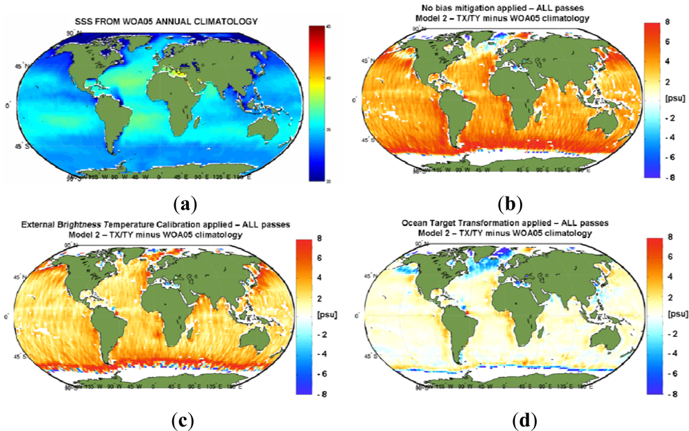
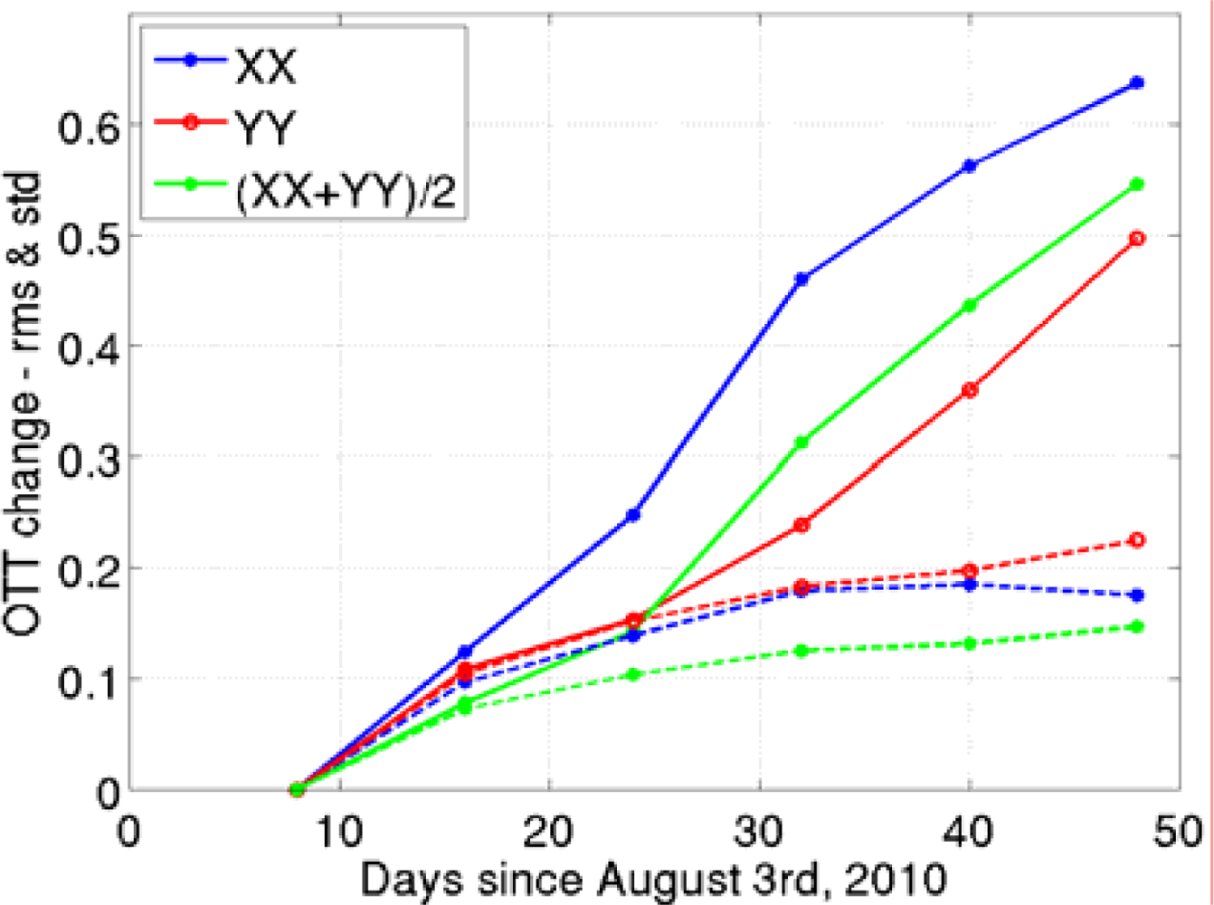
3.2. The Ocean Target Transformation

Biases in salinity retrievals from SMOS may be of instrumental origin (e.g., the residual calibration bias in the Noise Injection Radiometer [45]), induced by an imperfect correction of the foreign sources (e.g., cosmic background, errors in the brightness temperature of the Sun being subtracted) [4648], or dependent on the scene being imaged, which is the case of residual multiplicative amplitude and phase errors [25,49]. Biases can also be introduced by the differences in the dielectric constant models used to simulate the flat sea contribution [5053], or by the models describing the impact of sea state on the brightness temperature [54]. Therefore, bias mitigation is essential for accurate salinity retrievals and its validation can be performed using level 3 (L3) salinity products.
Despite the substantial progress in the instrument calibration, improvement on the detection of instrument and image reconstruction TB biases over the oceans remains critical. In fact, systematic antenna-based error patterns have been detected in SMOS TB measurements at X-pol (TX), Y-pol (TY), and Stokes’ third and fourth parameters, as already foreseen in [42]. These error patterns have typical amplitude of ±5 K (e.g., see Figure 1 of [55]). They have different possible sources: residual antenna pattern misestimates for the different receivers, the image reconstruction procedure itself and calibration residual errors.
Two bias-removal methods have been tested:
  • The external brightness temperature calibration, in which an average TB is computed in the field of view using some a priori geophysical parameters, and this value is subtracted from the average TB measured in the field of view [42].
  • The Ocean Target Transformation (OTT) [56,57] is computed from the average TB departure from a forward model (model-dependent) [55]. In line with the L2OS, errors are assumed to be additive in the OTT computation so far.
In order to perform the bias mitigation, a large ensemble of actual L1B SMOS data is required. All available data from ascending passes in 30 days (from 3 August to 2 September 2010; L1 Operational Processor v3.4.5) have been filtered to select pure ocean scenes, discarding snapshots contaminated by reflected galactic plane, and detecting the presence of land at L1B also in the aliases regions (L1C is not useful, since it does not contain the alias regions). Data selection to homogenize the observed geophysical conditions within the FOV, and to reduce the number of sources of variability has been performed, by automatically identifying and removing outliers.
Figure 6 [58] presents the World Ocean Atlas 2005 (WOA05) climatology [59], and the L3 10-day map minus the WOA05 climatology for the nominal case (no bias mitigation applied), for the external TB calibration, and for the model-dependent OTT assuming model 2 of the L2OS processor (Small Slope Approximation method or SSA [8]), in dual polarization obtained from full-polarimetric data, third and fourth Stokes parameters neglected.
As it can be appreciated, without any bias mitigation, retrieved salinities are positively biased. In the external TB calibration the bias is reduced, but not cancelled, and strips are visible in the retrievals (Figure 6(c)) due to the small, but non-negligible, biases between adjacent overpasses. These features are not visible with the OTT (Figure 6(d)) which only exhibits biases in high wind regions and in the North Pacific and Atlantic due to the RFI created by the long-range radars.
The quality of the retrieved geophysical parameters strongly improves when the OTT is applied, while much work is still required to improve the estimation of these systematic patterns. An intrinsic assumption of this approach is that these instrumental errors are systematic and therefore stable (invariant) in time and space. Nevertheless, imperfections in instrument calibration, data processing, OTT formalism, external noise sources (Sun, galaxy, etc.) introduce variability in the images, misleading the systematic instrumental pattern estimation. OTT inaccuracies propagate down to the retrieved salinities and, as such, are very important to assess and reduce. The OTT stability assumption was used to evaluate the quality of the OTT in [60].
In Figure 7 (from [60]), several OTTs are computed in temporal windows of eight days. The plot shows the increasing OTT mismatch as a function of time (using the OTT for first temporal window as reference), up to 0.6 K root mean square (rms). It was checked that most of this r.m.s increase is explained by an increasing (negative) bias, while the standard deviation (SD) remains rather constant (around 0.15 and 0.2 K for 1st Stokes and TX or TY, respectively) over the entire period. Such negative bias increases (in absolute value) at a rate of about 0.4–0.5 K per month. It is highly consistent with recent diagnostics on the drift induced by the Flat Target Response (FTR): several sky images were reconstructed after FTR correction and results showed that, with increasing lag between sky images and FTR acquisition dates, a negative drift of the order 0.5 K per month appears in the centre of the image.
Originally, the salinity retrieval processing at the SMOS Data Processing Ground Segment (DPGS) used a unique OTT provided as a fixed auxiliary file, and the results showed that 0.5–0.6 K discrepancy can be expected at several weeks interval, which should propagate to salinity biases of the order of 1–1.2 psu. The results also suggested that periodic OTT updates should help in reducing the SSS temporal biases. Moreover, Figure 7 provides a useful metric to define the optimal periodicity of the OTT update. The current DPGS updates the OTT on a monthly basis.
Besides temporal OTT errors, geographical (latitudinal) errors of the order of ±0.6 K have been identified, both in the OTT estimates and the inversed salinities [60]. Part of these errors is likely to be due to imperfect foreign sources corrections [46,47], which are currently under analysis. As such, these errors are expected to be significantly reduced in future versions of the processors. Another part is likely to be due to forward model inaccuracies [54]. To improve its accuracy, longer and stable datasets are required to infer semi-empirical models [61]. However, to separate foreign source-induced variability from model error-induced variability, it is desirable to reduce the impact of models in the OTT estimate. Such work is in progress and preliminary results have already been presented [55].
More recently, multiplicative (rather than additive) OTTs have been proposed as a way to mitigate even further the effect of instrument errors in the TB maps [62]. The performance of this new technique is still under evaluation.

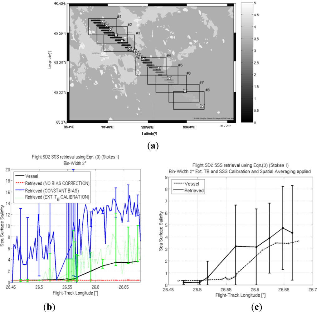
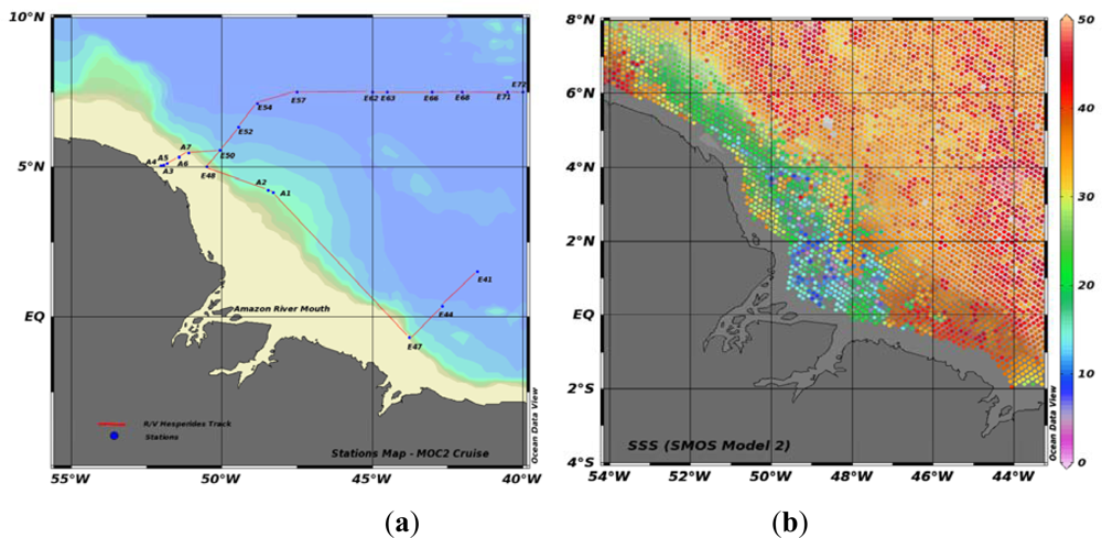
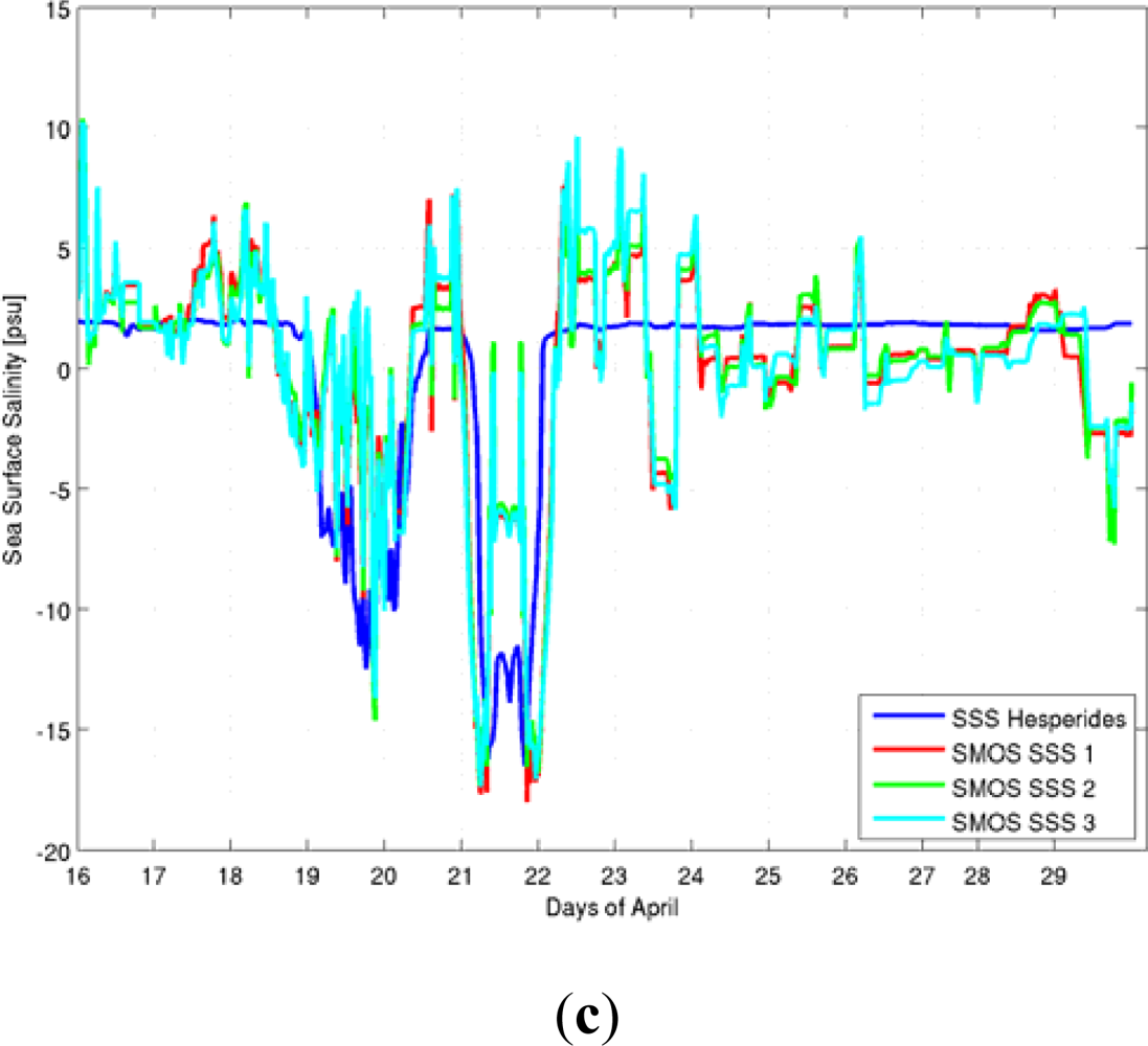
3.3. Validation of SMOS Salinity Products by in situ Oceanographic Measurements

The validation of preliminary SMOS salinity products at L1 and L2 is done against in situ data (from Argo floats or surface drifters) and various SSS products as, for example the WOA05 climatology [59], The validation strategies are: (a) statistical analysis of the differences between SMOS salinity retrievals and the available in situ observations; and (b) reproduction of spatial (or temporal) features. Both strategies are complementary because SMOS only senses the uppermost 1 cm of the ocean [63], while most of the in situ measurements are taken at deeper depths (0.5–5 m below the surface). The SMOS L2 salinities, binned in 0.5° by 0.5° boxes, have been compared with the vertically interpolated Argo data at 7.5 m below the surface (to avoid some of the incorrect behavior of the uppermost salinity measurements from Argo). The results correspond to August 2010 and all valid (global) Argo surface data floats. All regions were taken, the retrieved SSS has a fresh bias of 0.01 psu. The rms of the differences is about 0.7 psu, comparable to the global estimate given by [14]. Although these values are larger than the salinity differences between the 0–5 m and the 5–10 m measured by [64], it is expected that these statistics may improve by using in situ measurements as close as possible to the surface. To this end, we developed a prototype of surface drifter able to carry a highly precise conductivity-temperature probe at 0.5 m below the surface (Figure 8) and transmit the data in real or near-real time [65]. After being tested in different environments, a large number of units were built and were started to be released early in 2011 in several ocean regions (N Atlantic, S Atlantic, S Indian, and Equatorial Pacific) for future use in SMOS validation.
The results presented here include the experimental data obtained during the MOC2 (Meridional Overturning Circulation—Memory of the Climate) cruise, held from 4 April to 20 May 2010, departing from Fortaleza (Brasil) to Mindelo (Cabo Verde) on the research vessel Hespérides of the Spanish Navy. In situ measurements included water samples for sea surface salinity, CDOM (chromophoric dissolved organic matter) analyses from absorbances at 340 and 443 nm, FDOM (fluorescent dissolved organic matter) analyses, and SSS values for the whole cruise from thermo-salinograph. Also, SeaWIFS L2 absorption coefficient and SMOS L2 SSS maps remotely sensed data were acquired.
Figure 9 presents the track of the Hespérides, together with the SMOS-derived SSS map using model 2, and the salinity anomalies in the vessel transect. As it can be appreciated, SMOS data are already able to reproduce spatial features. No significant differences appear between the three different SSS retrievals with SMOS and Hesperides’s thermo-salinograph, except maybe in the crossings with the Amazon plume due to the different sampling depths [66].

3.4. Assessment of SSS Error Sources in a Numerical Model Regional Simulation

High-level salinity products (L4) may be obtained by means of data assimilation of SMOS salinity observations onto a numerical ocean model. Data assimilation methods derived from the Kalman Filter [67] are based on the weighted average of the output of the model and the observations. The weights are a function of the respective errors. To estimate the error of the SSS of a given numerical ocean model, as well as to identify the main sources of error, a numerical simulation study has been performed.
The model used in this study is the free surface OPA9.0 Ocean General Circulation Model [68]. It solves the Primitive Equations discretized on a C-grid centered at tracer points (temperature and salinity), and uses z-coordinates in the vertical. The regional configuration over the eastern part of the North-Atlantic Ocean requires four open boundaries (Figure 10(a)). The atmospheric forcing fields come from the ECMWF-ERA40 reanalysis. Further details of the simulation are in [69] and [70]. Assuming that the mixed-layer (defined as the 0.01 kg·m−3 density criterion) average of salinity is a proxy for SSS, the salinity budget is estimated. The contributions taken into account in the model are the integrated zonal, meridional, and vertical advection terms, the lateral and vertical diffusion, the surface freshwater evaporation and precipitation and river runoff, and the entrainment due to the variation of the mixed layer depth.
Sensitivity experiments, measuring the impact of the various processes to the resulting SSS are performed by modifying model parameters and atmospheric data. In these experiments, a 15-year reference simulation is compared with various 15-year simulations that differ by one of these various parameters.
The results shown in Figure 10(b) are separated in two families: the six experiments at left of the plot represent the impact of errors in the forcing fields (switching from the reference ECMWF forcing field to the equivalent NCEP product). The vertical black lines represent the relative magnitude of the difference between both fields. It is calculated as the spatial r.m.s. of the difference of the long term mean of both fields, divided by the spatial standard deviation of the long term mean of the reference field. The key of the first six experiments shown in Figure 10b is as follows: experiment “τ” represents the experiment where the ECMWF atmospheric wind stress, used for the transfer of momentum, is substituted by the one from NCEP. In experiments “W”, “H”, “T”, and “P” the surface wind speed (used for the heat fluxes calculation), the air humidity, the air temperature, and the precipitation are changed, respectively. Finally, in the experiment “O”, the data of temperature, salinity and horizontal velocities upon the open boundaries are modified. The reference simulation uses boundary data from the MERCATOR service ( http://www.mercator.eu.org/), the new simulation uses boundary data from a simulation of the North Atlantic Ocean. The results indicate that the change in the annual mean of the SSS is the largest when the surface wind stress and the ocean open boundary data are modified. In other terms, the largest sources of errors in SSS are the errors in the wind stress and in the open boundary data. Of note is that precipitation, usually considered as a source of uncertainty in the model SSS, while it does indeed play a significant role on the SSS, has a much weaker impact than that of the wind stress.
The final set of experiments shown in Figure 10(b), illustrate how the SSS change in response to changes in some model parameters and model parameterizations: Changing from bi-Laplacian horizontal viscosity to a Laplacian one is indicated by “V”; changing the Laplacian diffusion coefficient of salinity is indicated by “L”; changing the vertical mixing scheme (from the TKE to the Richardson-number dependent scheme) is indicated by “M”; switching-off double diffusion parameterization and river-runoff is noted by “D” and “R”, respectively; switching-on the Newtonian relaxation of SST and SSS towards their climatic values are noted by “τt” and “τs”, respectively.
It can be seen that switching-on relaxation towards climatology and the changes in the lateral salt diffusivity, trigger the largest impact on SSS. While the Newtonian salinity relaxation provides a direct impact through the establishment of an artificial freshwater flux, temperature relaxation changes the surface heat fluxes that affect SSS via evaporation changes.
These results are easily exploited in Ensemble Kalman Filter data assimilation by enhancing the spread of a set of model states (used as proxy of the model error) if each ensemble member is driven by a slightly different surface wind stress, and/or they differ in the value of the saline diffusivity coefficient. Salinity products (L4) may be obtained by means of data assimilation of SMOS salinity observations onto a numerical ocean model. Data assimilation methods derived from the Kalman Filter [67] are based on the weighted average of the output of the model and the observations. The weights are a function of the respective errors. A numerical simulation study has been performed to estimate the error of the SSS of a given numerical ocean model, as well as to identify the main sources of error.

4. Soil Moisture Downscaling Algorithms

For land applications, SMOS spatial resolution is adequate for improving our understanding of water and energy fluxes between the atmosphere, the soil surface, and subsurface. However, it is insufficient for regional applications, such as land and water resources management, agricultural productivity, weather and climate forecasting, and flood and drought mitigation, which require a spatial resolution of 1 to 10 km. Hence, within SMOS preparatory activities, the possibility of improving the spatial resolution of SMOS observations by using pixel disaggregation techniques with optical and infrared data at a much higher resolution was explored to overcome the limitations of the existing disaggregation schemes [71]. Different downscaling experiments were carried out at the REMEDHUS calibration and validation site, within the GRAJO (GPS and Radiometric Joint Observations) long-term field experiment, using airborne passive observations acquired with the UPC Airborne RadIomEter at L-band (ARIEL) and LANDSAT imagery. Results from these downscaling activities are presented in Section 4.1.
Following the SMOS launch, and based on the experience gained from the downscaling activities with airborne data, a downscaling strategy for the estimation of high resolution soil moisture from SMOS using MODIS visible/infrared (VIS/IR) data was developed. This algorithm is an extension of the so-called “universal triangle” concept that relates VIS/IR parameters, such as the Normalized Difference Vegetation Index (NDVI), and Land Surface Temperature (Ts), to the soil moisture status. It combines the accuracy of SMOS observations with the high spatial resolution of visible/infrared satellite data into accurate soil moisture estimates at high spatial resolution. As a first validation exercise, the method was applied to a set of SMOS images acquired during the commissioning phase over South-Eastern Australia, providing first evidence of its capabilities. An overview of the downscaling method proposed for SMOS and the results obtained in this validation exercise are provided in Section 4.2.
At the SMOS-BEC (SMOS Barcelona Expert Centre on Radiometric Calibration and Ocean Salinity), this downscaling approach has been implemented to provide SMOS-derived 1 km soil moisture maps as a value-added product. Experimental 1 km soil moisture maps of the Iberian Peninsula are provided through the SMOS-BEC web site ( http://tarod.cmima.csic.es/), and present efforts involve evaluating the performance of the algorithm over a wide variety of land covers and climate conditions. Sample 1 km soil moisture maps resulting from the application of the algorithm using SMOS L2 data v.4.0 are shown in Section 4.3.

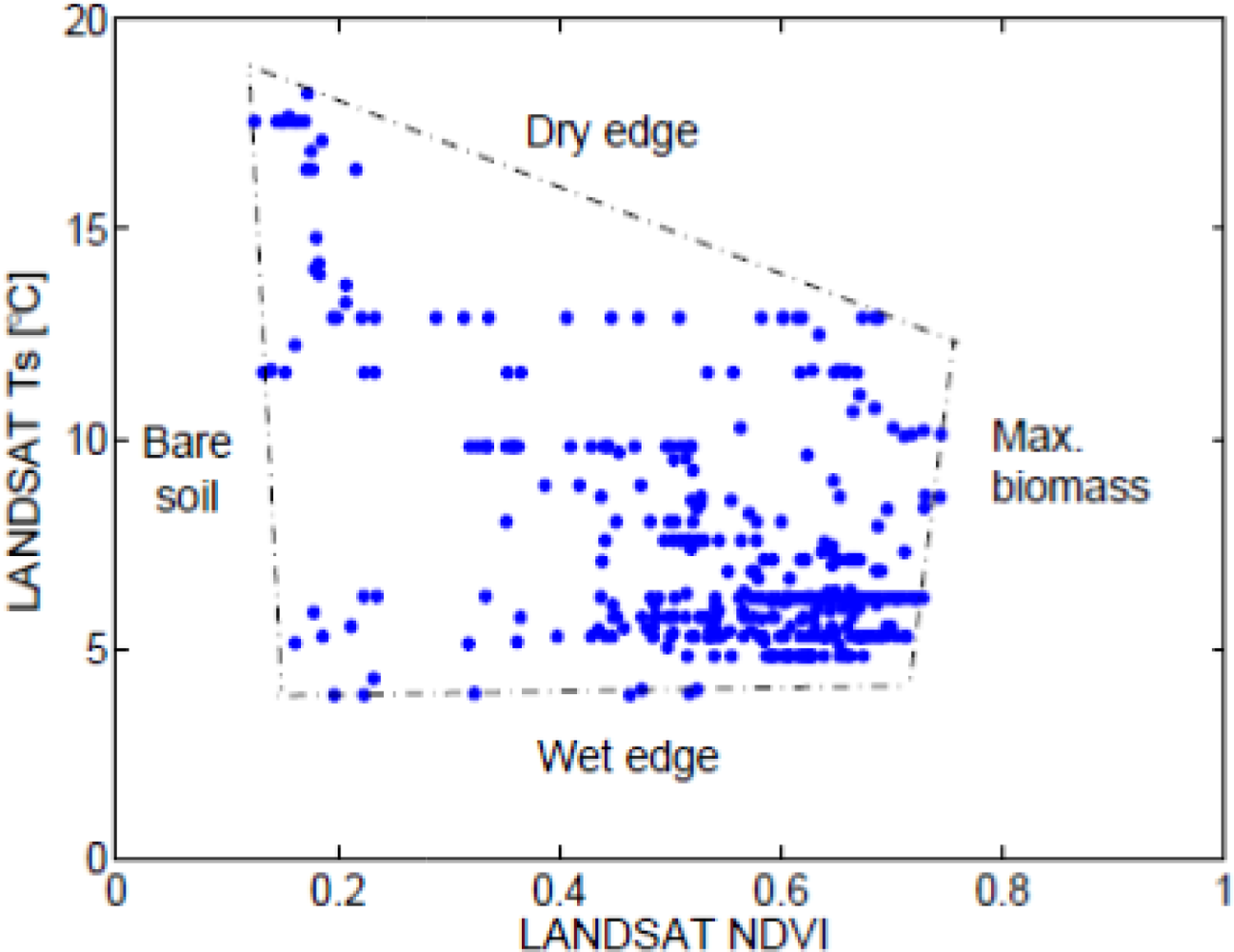
4.1. Downscaling Approach for Airborne Data at the REMEDHUS Site

These activities were performed in the frame of the GRAJO (GPS-R and RAdiometry Joint Observations) field experiment, a joint venture between UPC and the Centro Hispano Luso de Investigaciones Agrarias (CIALE)/Universidad de Salamanca (USAL) in support of the SMOS calibration/validation activities The experiment was conducted at the REMEDHUS soil moisture network in the semi-arid area of the Duero basin, Zamora, Spain, from November 2008 until May 2010. It is an area of approximately a SMOS pixel (40 × 30 km), quite homogeneous (mostly covered by crops), and equipped with a complete and operational network of 23 soil moisture and temperature sensors (see Figure 11). Its climate is continental and semiarid, with cold winters and warm summers (12 °C annual mean temperature and 400 mm mean rainfall).
Flights at different altitudes were performed over the REMEDHUS site with the UPC Airborne Radiometer at L-band (ARIEL) [72] and a downscaling algorithm to improve the spatial resolution of ARIEL-derived soil moisture using higher resolution LANDSAT imagery was evaluated. Radiometric measurements were acquired during two flights undertaken on 25 March 2009, one in the morning right after sunrise (Flight 1), and one in the evening right before sunset (Flight 2), covering an area of ∼720 × 720 m each. Figure 12 shows the antenna temperature maps from the two flights, overlapped in an aerial photography from Google Earth. These measurements were obtained at heights 140 ± 30 m. As a rule of thumb, ARIEL observations have a footprint of approximately 1/3 times the flight height; accordingly, ARIEL TB on Figure 12 has a pixel size of ∼50 m. However, since ARIEL data will be jointly used with LANDSAT data at a spatial resolution of 30 m, ARIEL observations have been conveniently resampled to a 60 × 60 m grid.
A LANDSAT 5 satellite image from 23 March 2009, scene 201/031, radiometrically and geometrically corrected using ten ground control points was used in this study. The NDVI of the area under study was obtained from the surface reflectance of bands 4 (Near-infrared, 0.76–0.90 μm) and 3 (Visible, 0.63–0.69 μm), respectively, at 30 m spatial resolution. The surface radiant temperature (Ts) of the area under study was from band 6 (Thermal, 10.40–12.50 μm) at 120 m spatial resolution, re-sampled to 30 m.
The downscaling approach adopted in these airborne activities consists of aggregating high resolution VIS/IR land surface parameters (particularly, LANDSAT Ts and NDVI) to the scale of ARIEL radiometric observations for the purpose of building a linking model that is afterwards applied at fine scale to disaggregate the passive soil moisture observations into high-resolution soil moisture.
A number of studies have documented the emergence of a triangle of trapezoidal shape when remotely sensed Ts over heterogeneous areas are plotted against Vegetation Index (VI) measurements (e.g., [73]). Figure 13 illustrates the polygonal correlation between LANDSAT Ts and NDVI on Flight 1. The polygon’s edges can be interpreted as the minimum/maximum reached by vegetation cover (NDVI) and soil moisture. The warm edge of the triangle is generally interpreted as representing limiting conditions of soil moisture or evapo-transpiration, in contrast to the cold edge, which represents maximum evapotranspiration and thereby unlimited water access. Therefore the warmest and coldest pixels are usually referred to as the dry and wet edges of the triangle, respectively. As a first approach, the “universal triangle” concept developed by [73] was directly used as the basis to define the linking model:
s m = i j k a ijk NDVI i T Sr j .
The following approximation of Equation (1) was chosen as a linking model to relate the Landsat Ts/NDVI space to airborne soil moisture estimates: and normalized Ts (TN) and NDVI (fractional vegetation cover, Fr) between its maximum and minimum values.
s m = a 00 + a 01 T N + a 10 F r + a 11 T N F r + a 02 T N 2 + a 20 F r 2
where TN and Fr (fractional vegetation cover) are the normalized LANDSAT Ts and NDVI between its maximum and minimum values.
Ground measurements of 0–5 cm soil moisture at 20 sampling locations were acquired simultaneously with the airborne observations. ARIEL-derived soil moisture was retrieved from ARIEL TBs through linear regression with in situ soil moisture samples (correlation coefficients equal to 0.78 and 0.57 for Flights 1 and 2, respectively). The lower correlation on Flight 2 is probably due to its acquisition time (4.45 PM), which is far from LANDSAT overpass time (10.40 AM) and therefore can induce significant errors on Ts.
Figure 14 shows the ground-based soil moisture maps (from spatial kriging of soil moisture measurements, left column), the ARIEL-derived soil moisture (from linear regression with in situ samples, second column), the down-scaled soil moisture (from the application of the downscaling method, third column), and their associated errors (fourth and fifth columns, computed as first column minus the second, and first column minus the third one, respectively). From the comparison with ground-based soil moisture values, it can be seen that the ARIEL-derived and the downscaled images reproduce the spatial variations in the soil moisture measurements. The spatial distribution of the r.m.s. error between ARIEL-derived soil moisture and ground-based soil moisture is improved by a ∼40%, when the downscaling method is applied.

4.2. Downscaling Approach for SMOS

A downscaling approach for SMOS using MODIS Ts and NDVI data was developed using the same downscaling strategy as in Section 4.1. For the SMOS case, in addition to the linking model shown in Equation (2), an extension of the triangle concept was used to define a novel linking model which strengthens the relationship between MODIS-derived land surface parameters and SMOS soil moisture retrievals. This model is a regression formula that relates the SMOS L2 soil moisture estimates (sm) and SMOS L1c brightness temperatures, with the LANDSAT NDVI and Ts aggregated at ARIEL's resolution (Equation (1)) [74].
s m = a 000 + a 001 T BN + a 010 T N + a 100 F r + a 002 T BN 2 + a 020 T N 2 + a 200 F r 2 + a 011 T N T BN + a 101 F r T BN + a 110 F r T N ,
where TBN = (TBTB,min)/(TB,maxTB,min) is the normalized SMOS L1c TB at H-polarization and 42.5 °C, TN = (TSTS,min)/(TS,maxTS,min) is the normalized surface temperature, and Fr = (NDVINDVImin)/(NDVImaxNDVImin) is the normalized NDVI.
Using Equation (3) a system of equations is defined for all image pixels, and the regression coefficients aijk are retrieved. In principle, these coefficients are region- and time-dependent, and studies are being performed to analyze the goodness of global coefficients. Once the aijk coefficients are known, high resolution soil moisture maps are then obtained from Equation (3), using the high resolution TN and Fr, and the low resolution TBN resampled at the high resolution grid.
Following the SMOS launch, the downscaling algorithm was applied to a set of SMOS images acquired during the commissioning phase over the Murrumbidgee catchment, in South-Eastern Australia, and validated with the in situ data from the OZnet soil moisture monitoring network [75]. Figure 15(a) shows the Murrumbidgee catchment elevation with dots indicating the location of the permanent soil moisture monitoring, and rectangles demarcating its intensive study areas. The comparison of downscaled soil moisture estimates to ground-data was focused on a subset of those stations within the Yanco region (Figure 15(b)). The temporal evolution of soil moisture measurements and daily rainfall observed at Yanco monitoring stations is shown in Figure 15(c).
Figures 16 shows visual results of the application of the proposed downscaling algorithm to SMOS data acquired on 17 February 2010 (6 AM). The different panels show in the top row the SMOS L2 soil moisture [m3/m3] on a 40 km × 40 km grid and the 1 km SMOS-derived soil moisture maps [m3/m3] using the universal triangle approach, and the proposed extension as linking model, and in the bottom row the SMOS brightness temperatures at horizontal polarization and 42.5° incidence angle, the 1 km MODIS/AQUA surface temperature, and the 1 km MODIS/TERRA NDVI. Results show that the use of brightness temperatures in the linking model is needed to capture the soil moisture variability on the finer scale, and to reproduce changes in soil moisture due to rain events being detected by SMOS at 6 AM, but not by MODIS/TERRA at 10.30 AM or MODIS/AQUA at 1.30 PM. Results from comparison with in situ data indicate that soil moisture variability is effectively captured at 1 km scale without a significant degradation of the rms error [75].

4.3. High Resolution Soil Moisture Maps: SMOS-BEC Research Product

This downscaling approach is now being applied to different regions world-wide to assess its goodness over a wide variety of land covers and climate conditions. At present, experimental 1 km soil moisture maps of the Iberian Peninsula are provided at the SMOS Barcelona Expert center. Figure 17 shows results of the application of the proposed downscaling algorithm to a SMOS image over the Iberian Peninsula, from 22 August 2011.
These high resolution soil moisture maps as well as sea surface salinity maps at 3 days/1°, 10 days/0.5°, and optimally interpolated SSS maps at 10 and 30 days, can be downloaded from the SMOS-BEC data distribution and visualization service: http://tarod.cmima.csic.es/ncWMS/. Future activities will include the extension to other geographical areas, the use of daily NDVI, and the possibility of retrieving high resolution soil moisture estimates in the areas where clouds are masking MODIS measurements.

5. Preparatory Activities to Improve the Performance of Eventual SMOS Follow-on Missions

In this section we briefly summarize the main outcomes of the activities conducted to assess the goodness of GNSS-R techniques to perform a better sea state correction and therefore, improve the sea surface salinity estimates from SMOS, and to infer soil moisture and vegetation parameters.

5.1. Application to Sea State Correction

The underlying concept under the use of GNSS-R is simple: when the electromagnetic wave is scattered over the sea surface, the scattered signal changes its polarization (from RHCP to mostly LHCP) and arrives at the receiver mainly from the specular reflection point, determined by the shortest distance between the transmitting GPS satellite and the receiver. However, as the sea becomes rough, the scattered signals come from a wider region (known as “glistening zone”) that enlarges with increasing roughness, in a similar manner as the Sun reflecting over the sea.
In classical GNSS-R, observables are derived by cross-correlating the received scattered signal with a local replica of the pseudo-random noise signals (open C/A code in the case of GPS) transmitted by the navigation satellites, generated at different delays and Doppler frequency shifts. Actually the values of this two-dimensional cross-correlation are called the Delay-Doppler Map (DDM), which looks like the function shown in Figure 18. When the sea gets rougher, the volume under the normalized DDM (peak equal to 1) down to a predetermined threshold above noise level, increases as well.
The field experiments ALBATROSS 2008 and 2009 performed in the Gran Canaria island (Figure 19(a)) demonstrated that the changes in the brightness temperatures at different polarizations and incidence angles were correlated to the changes in the volume of the DDM (Figure 19(b)), and that this information could be used in a synergetic way to correct for the sea state [76,77].
Actually, it was also found that the length of the tail of the waveform (cut of the DDM for Doppler shift equal to 0 Hz) at 1/e was also highly correlated to the sea state. These results have also been used in COSMOS-OS data [78] to improve the salinity retrievals [79]. The experiment conditions are those of Figure 5, and results are shown in Figure 20: blue dots represent the retrieved salinity without any correction, green dots represent the retrieved salinity with the GNSS-R-derived correction, and the red dots are, as a reference for the error introduced by the retrieval algorithm, the SSS retrieved from the flat sea model and the ground-truth measurements. These are very encouraging results, since the instruments were different (the UPC griPAU instrument [80] used in ALBATROSS, and the IEEC GOLD-RTR instrument [81] in COSMOS-OS), and the sea state conditions were totally different. More details can be found in [77,79].

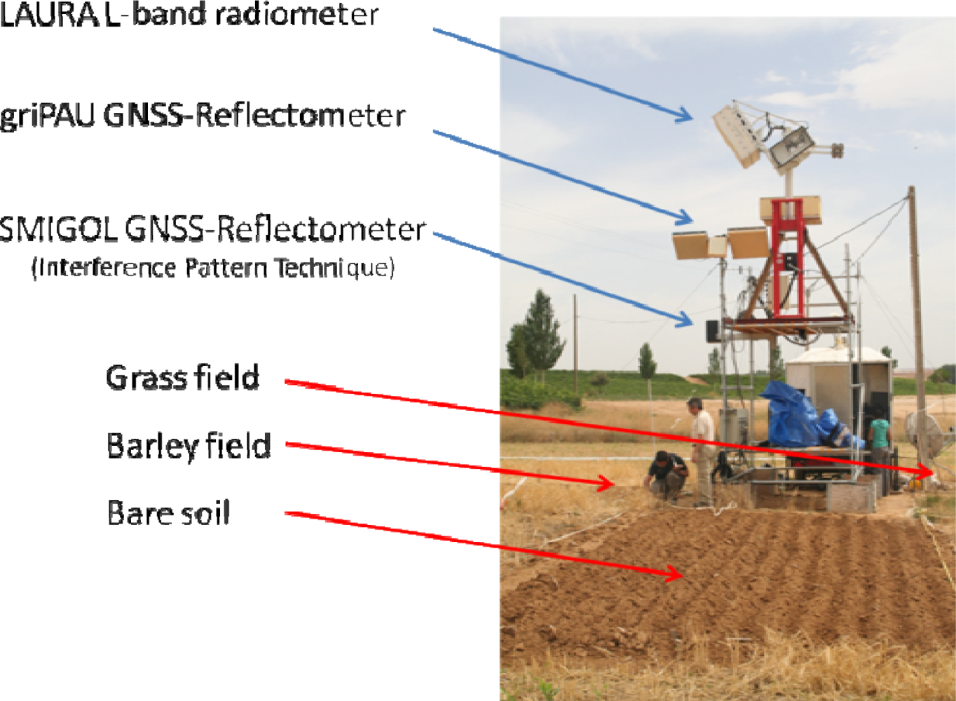
5.2. Application to Soil Moisture Monitoring

In the GRAJO field experiment, UPC was in charge of the ground-based (LAURA radiometer [82]) and airborne (ARIEL radiometer [72]) L-band radiometric data and the GNSS-reflectometer data acquisitions with the griPAU [80] and SMIGOL [83] instruments, the first one implementing the classical GNSS-R approach, and the second one the so-called interference pattern technique. Figure 21 shows the ground-based microwave instrumentation installed in a 3 m high scaffolding.
During the GRAJO experiment the griPAU instrument confirmed that the reflected GPS signal was nearly specular, and the peak amplitude of the DDM was highly correlated to the surface’s soil moisture [84], as shown in Figure 22(a, b). Figure 22(a) shows the geolocated peak (in arbitrary units) of the DDM as the specular reflection points moves with the GPS satellite movement in the bare soil field, while Figure 22(b) shows the associated soil moisture map measured with the Theta Probes [85] over a dense grid of sampling points. The qualitative agreement between both images is very good, and the quantitative analysis presented in Figure 22(c) shows a strong correlation between these two data sets (r = 0.87) for soil moisture values larger than ∼10%. Despite the excellent sensitivity of the griPAU instrument, which was able to observe and track the changes associated to the navigation bit in the reflected signal over the sea surface during ALBATROSS 2009, for soil moisture values below 10%, the reflection coefficient decreases and the amplitude of the DDM peak becomes too noisy to be accurately estimated.
The results presented in Sections 5.1 and 5.2 are very promising, since they prove the concept of using GNSS-R techniques over the oceans to improve the accuracy of the SSS retrievals, by performing the required sea state correction of the brightness temperatures, while over land they are sensitive to soil moisture.

6. Summary and Conclusions

A review of the recent results obtained by the CALIMAS team in preparation to and during the SMOS calibration/validation activities has been presented. A number of CALIMAS-related studies focused on improving the quality of the SMOS TB images and the subsequent SSS retrievals.
Using the UPC MIRAS Testing Software, the team assessed the planned internal and external radiometer calibrations and contributed to the definition of the optimum instrument calibration strategy. As a drift on the MIRAS PMS offset was identified, a new antenna physical model was proposed to take into account temperature effects at orbital and seasonal scales. These results have led to improvements in the SMOS L1 processor ingested in the DPGS production chain in October 2011. In parallel, image reconstruction algorithms capable of automatically detecting and largely mitigating the presence of RFI (point and extended sources) have been developed and tested.
The performance of salinity retrieval algorithms was tested prior to launch with the existing airborne two-dimensional synthetic aperture radiometers: ESA’s SMOSillo over Lake Lojha, West of Helsinki, Finland, and Aalto University’s HUT-2D over the Baltic Sea. These tests facilitated the identification of problems that were later found in SMOS measurements (as for example the presence of bias in the data, and the correction of the sea state impact on the TB) and focused efforts in finding solutions for them: for example the TB and SSS calibrations, and use of GNSS-R information to correct for the sea state.
The performance of SMOS salinity retrieval algorithms was evaluated. To mitigate residual biases at L1, an Ocean Target Transformation (OTT) was proposed [56,57] and implemented in the L2OS [86]. The team assessed the optimal strategy to perform the OTT in operations. In the assessment, the need for careful data selection and a periodic computation of the OTT is thoroughly addressed. The recommendations of this study are now being implemented in operations (version 5.00) and are planned to be used in the next SMOS reprocessing campaign (end of 2011). Another relevant outcome of this study is that the quality of the OTT is limited by the uncertainties of the forward model used in its computation. In particular, uncertainties in, e.g., the sea surface roughness and galactic modeling are projected onto the OTT and therefore the SSS retrievals. The CALIMAS team has been working on an alternative method, based on careful selection of the mean geophysical conditions in the antenna reference frame to build a bias correction independent of any full forward model [55]. This is now being finalized, validated and compared to other approaches for an eventual implementation into an improved future version of the L2OS processor. Another method for improvement of TB images, based on multiplicative rather than additive corrections, is also currently under evaluation [62]. Moreover, recent OTT developments have led to an improved empirical sea surface roughness model [61], which was introduced in 2011 as one of the three alternative roughness correction formulations in the SMOS operational L2OS processor (version 5.00). The scene dependent bias correction that uses the external TB calibration and that was proposed by [42] before the SMOS launch, was initially discarded for the L2OS processor (since it used non-SMOS information) and may now be reconsidered to improve the correction of the still existing residual land contamination over the ocean [13,14].
Salinity retrievals have been validated using Argo upper surface salinity values and using surface drifters observations from a field experiment aboard the Hespérides research vessel, in a transect from Brazil to Cabo Verde. The rms between the preliminary salinity retrievals and the Argo data is of about 0.7 psu. This value, representing the global distance between the two estimations of the SSS is compatible with the value of other authors [14]. On the other hand, prototype drifters, measuring salinity close to the ocean surface, have been designed and built by the SMOS-BEC, and a number of units were later released (2010–2011) in the Atlantic, Indian and Pacific oceans for future fine tuning of the SMOS SSS products validation in coordination with other cal/val teams.
The impact of different sources of sea surface salinity errors in numerical models has also been investigated. This study is important for the generation of L4 salinity products from SMOS as data assimilation is one of the two main strategies (together with data fusion) to provide geophysically coherent maps of salinity. It was found that the largest relative sources of errors are the forcing fields of surface wind stress, precipitation, and data in the open boundaries.
Although the main focus of activity of the SMOS-BEC (to which most of the authors of this paper belong) is the instrument calibration and the retrieval of salinity, the interests and the objectives of CALIMAS also cover land applications. The Spanish SMOS high level processing center CP34 now distributes SMOS L3 maps of soil moisture, vegetation water content and dielectric constants over land, but also envisages offering tailor-made added-value L4 products for specific applications.
A technique to disaggregate mixed pixels down to 1 km SMOS using MODIS VIS/IR information has been proposed. This technique has been validated using the network of soil moisture probes of the Yanco site, in the Murrumbidgee catchment (Australia) and was recently applied to identify fire outbreaks in Spain. Further validation exercises are underway to evaluate the performance of the algorithm over a wide variety of land covers and climate conditions. An application now under development uses these high resolution maps to evaluate the risk conditions for forest fires in Spain. This line of research should help to increase the value of SMOS as an Earth explorer, by going beyond the expected mission objectives supported by ESA and opening new possibilities for the research and application communities.
Finally, as a prospect for secondary payload for an eventual future SMOS-like mission, the use of GNSS-R auxiliary information to improve the quality of the SMOS retrievals has been studied. This is a promising new field of research that exploits opportunity signals provided by navigation satellites as additional data to complement the MIRAS radiometric measurements. Over the ocean, the UPC griPAU instrument was used in a ground-based field experiment to infer the relationship between the TB changes and the DDM volume (or length of the tail at 1/e). COSMOS-OS airborne data gathered using TUD’s (Copenhagen, Denmark) EMIRAD (an L-band real aperture radiometer) and IEEC’s (Barcelona, Spain) GOLD-RTR (a GNSS-Reflectometer) has been processed to infer sea state information and to improve sea state correction, with very promising results. Over land, griPAU-derived DDMs have validated the simple specular reflection model over the soil surface, since the shape of the DDMs does not distort (to measurements’ accuracy) in the scattering process. The correlation between the DDM peak amplitude and the soil moisture is excellent for soil moisture values above ∼10%. Below, the lower reflection coefficient, the peak amplitude reduces significantly. The inclusion of GNSS-R receivers as additional secondary payload in future SMOS follow-on satellites would improve one of the main problems in SMOS SSS retrieval: the lack of simultaneous roughness information to be included in the forward model (now relying on operational forecasts), and would also provide valuable additional information over land.
CALIMAS, from the calibration and validation perspectives, and the rest of SMOS-BEC activities will continue analyzing possible improvements to SMOS data processing, and providing insights into new SMOS-derived products and applications to be considered for implementation by CP34. Envisaged activities include the improvement of image reconstruction algorithms, especially in coastal regions, RFI detection and mitigation algorithms, calibration (alternative OTTs), forward modeling, salinity inversion algorithms, in addition to a detailed evaluation of SMOS salinity products quality and compliance with the requirements, and the study of the limits of the downscaling techniques over land. Data fusion methods are currently being tested building orders to develop, not only the mentioned L4 high resolution land products, but also improved salinity maps using information on ocean dynamics (flow characteristics) obtained from other satellite sensors.

Acknowledgments

This work has been performed under research grants TEC2005-06863-C02-01/TCM, ESP2005-06823-C05, ESP2007-65667-C04, AYA2008-05906-C02-01/ESP and AYA2010-22062-C05 from the Spanish Ministry of Science and Innovation, and a EURYI 2004 award from the European Science Foundation. Both UPC and ICM-CSIC have also been granted by ESA SMOS Expert Support Laboratory contracts for L1 and L2-ocean salinity during the reported period.

References

  1. Kerr, Y.H.; Waldteufel, P.; Wigneron, J.P.; Martinuzzi, J.M.; Font, J.; Berger, J.M. Soil moisture retrieval from space: The Soil Moisture and Ocean Salinity (SMOS) mission. IEEE Trans. Geosci. Remote Sens 2001, 39, 1729–1735. [Google Scholar]
  2. Font, J.; Camps, A.; Borges, A.; Martín-Neira, M.; Kerr, Y.H.; Hahne, A.; Macklenburg, S. The challenging sea surface salinity measurement from space. Proc. IEEE 2010, 98, 649–665. [Google Scholar]
  3. Kerr, Y.H.; Waldteufel, P.; Wigneron, J.P.; Delwart, S.; Cabot, F.; Boutin, J.; Escorihuela, M.J.; Font, J.; Reul, N.; Gruhier, C.; et al. The SMOS mission: New tool for monitoring key elements of the global water cycle. Proc. IEEE 2010, 98, 666–687. [Google Scholar]
  4. Mecklenburg, S.; Drusch, M.; Kerr, Y.H.; Font, J.; Martin-Neira, M.; Delwart, S.; Buenadicha, G.; Reul, N.; Daganzo-Eusebio, E.; Oliva, R.; Crapolicchio, R. ESA’s Soil Moisture and Ocean Salinity mission: Mission performance and operations. IEEE Trans. Geosci. Remote Sens, 2011; submitted. [Google Scholar]
  5. McMullan, K.; Brown, M.; Martin-Neira, M.; Rits, W.; Ekholm, S.; Marti, J.; Lemanczyk, J. SMOS: The payload. IEEE Trans. Geosci. Remote Sens 2008, 46, 594–605. [Google Scholar]
  6. Font, J.; Camps, A.; Ballabrera-Poy, J. Microwave Aperture Synthesis Radiometry: Setting the Path for Operational Sea Salinity Measurement from Space. In Remote Sensing of European Seas; Barale, V., Gade, M., Eds.; Springer-Verlag: New York, NY, USA, 2008; pp. 223–238. [Google Scholar]
  7. Kerr, Y.H.; Waldteufel, P.; Richaume, P.; Wigneron, J.P.; Ferrazzoli, P.; Mahmoodi, A.; Al Bitar, A.; Cabot, F.; Gruhier, C.; Juglea, S.; et al. The SMOS soil moisture retrieval algorithm. IEEE Trans. Geosci. Remote Sens 2012. [Google Scholar] [CrossRef]
  8. Zine, S.; Boutin, J.; Font, J.; Reul, N.; Waldteufel, P.; Gabarró, C.; Tenerelli, J.; Petitcolin, F.; Vergely, J.L.; Talone, M.; Delwart, S. Overview of the SMOS sea surface salinity prototype processor. IEEE Trans. Geosci. Remote Sens 2008, 46, 621–645. [Google Scholar]
  9. Yueh, S.H.; West, R.; Wilson, W.J.; Li, F.K.; Njoku, E.G.; Rahmat-Samii, Y. Error sources and feasibility for microwave remote sensing of ocean surface salinity. IEEE Trans. Geosci. Remote Sens 2001, 39, 1049–1060. [Google Scholar]
  10. Lagerloef, G.S.E.; Swift, C.T.; LeVine, D.M. Sea surface salinity: The next remote sensing challenge. Oceanography 1995, 8, 44–50. [Google Scholar]
  11. Wigneron, J.P.; Kerr, Y.H.; Waldteufel, P.; Saleh, K.; Escorihuela, M.J.; Richaume, P.; Ferrazzoli, P.; de Rosnay, P.; Gurney, R.; Calvet, J.C.; et al. L-band microwave emission of the biosphere (L-MEB) model: Description and calibration against experimental data sets over crop fields. Remote Sens. Environ 2007, 107, 639–655. [Google Scholar]
  12. Oliva, R.; Martin-Neira, M.; Corbella, I.; Torres, F.; Kainulainen, J.; Tenerelli, J.; Cabot, F.; Martin-Porqueras, F. SMOS calibration and performances after one year of data. IEEE Trans. Geosci. Remote Sens 2012. submitted.. [Google Scholar]
  13. Font, J.; Boutin, J.; Reul, N.; Spurgeon, P.; Ballabrera-Poy, J.; Chuprin, A.; Gabarró, C.; Gourrion, J.; Guimbard, S.; Hénocq, C.; et al. SMOS first data analysis for sea surface salinity determination. Int. J. Remote Sens, 2012; in press. [Google Scholar]
  14. Reul, N.; Tenerelli, J.; Boutin, J. Overview of the first SMOS sea surface salinity products, Part I: Quality assessment for the second half of 2010. IEEE Trans. Geosci. Remote Sens, 2012; submitted. [Google Scholar]
  15. Corbella, I.; Torres, F.; Duffo, N.; González, V.; Camps, A.; Vall-llossera, M. Fast Processing Tool for SMOS Data. Proceedings of the 2008 IEEE Geoscience and Remote Sensing Symposium, Boston, MA, USA, 7–11 July 2008; pp. 1152–1155.
  16. Corbella, I.; Torres, F.; Camps, A.; Colliander, A.; Martin-Neira, M.; Ribo, S.; Rautiainen, K.; Duffo, N.; Vall-llossera, M. MIRAS end-to-end calibration: Application to SMOS L1 processor. IEEE Trans. Geosci. Remote Sens 2005, 43, 1126–1134. [Google Scholar]
  17. Gutierrez, A.; Barbosa, J.; Almeida, N.; Catarino, N.; Freitas, J.; Ventura, M.; Reis, J. SMOS L1 Processor Prototype: From Digital Counts to Brightness Temperatures. Proceedings of the 2007 IEEE International Geoscience and Remote Sensing Symposium, Barcelona, Spain, 23–28 July 2007; pp. 3626–3630.
  18. Corbella, I.; Torres, F.; Duffo, N.; Martín-Neira, M.; González-Gambau, V.; Camps, A.; Vall-llossera, M. On-ground characterization of the SMOS payload. IEEE Trans. Geosci. Remote Sens 2009, 47, 3123–3133. [Google Scholar]
  19. Martin-Neira, M. Analysis of LO Phase Drift Calibration; SO-TN-ESA-PLM-6052; Technical Report; European Space Agency-European Space Technology Center (ESA-ESTEC): Noordwijk, The Netherlands, 2007. [Google Scholar]
  20. Ramos-Perez, I.; Bosch-Lluis, X.; Camps, A.; González, V.; Rodriguez-Alvarez, N.; Valencia, E.; Park, H.; Vall·llosera, M.; Forte, G. Optimum inter-calibration time in synthetic aperture interferometric radiometers: Application to SMOS. IEEE Geosci. Remote Sens, 2012. [Google Scholar] [CrossRef]
  21. Corbella, I.; Torres, F.; Duffo, N.; Gonzaìlez-Gambau, V.; Pablos, M.; Duran, I.; Martiìn-Neira, M. First Results on MIRAS Calibration and Overall SMOS Performance. Proceedings of the 11th Specialist Meeting on Microwave Radiometry and Remote Sensing of the Environment (MicroRad), Washington, DC, USA, 1–4 March 2010. [CrossRef]
  22. Brown, M.A.; Torres, F.; Corbella, I.; Colliander, A. SMOS calibration. IEEE Trans. Geosci. Remote Sens 2008, 46, 646–658. [Google Scholar]
  23. Camps, A.; Bará, J.; Corbella, I.; Torres, F. The processing of hexagonally sampled signals with standard rectangular techniques: Application to 2D large aperture synthesis interferometric radiometers. IEEE Trans. Geosci. Remote Sens 1997, 35, 183–190. [Google Scholar]
  24. Anterrieu, E. A resolving matrix approach for synthetic aperture imaging radiometers. IEEE Trans. Geosci. Remote Sens 2004, 42, 1649–1656. [Google Scholar]
  25. Camps, A.; Vall-llossera, M.; Corbella, I.; Duffo, N.; Torres, F. Improved image reconstruction algorithms for aperture synthesis radiometers. IEEE Trans. Geosci. Remote Sens 2008, 46, 146–158. [Google Scholar]
  26. Corbella, I.; Torres, F.; Camps, A.; Duffo, N.; Vall-llossera, M. Brightness-temperature retrieval methods in synthetic aperture radiometers. IEEE Trans. Geosci. Remote Sens 2009, 47, 285–294. [Google Scholar]
  27. Camps, A. Aplication of Interferometric Radiometry to Earth Observation. Ph.D. Thesis, Universitat Politècnica de Catalunya, Barcelona, Spain, 1996; Available online: http://hdl.handle.net/10803/6885 (accessed on 5 March 2012).
  28. Camps, A.; Corbella, I.; Bará, J.; Torres, F. Radiometric sensitivity computation in aperture synthesis interferometric radiometry. IEEE Trans. Geosci. Remote Sens 1998, 35, 680–685. [Google Scholar]
  29. Macelloni, G.; Brogioni, M.; Pampaloni, P.; Cagnati, A.; Drinkwater, M.R. DOMEX 2004: An experimental campaign at dome-c antarctica for the calibration of spaceborne low-frequency microwave radiometers. IEEE Trans. Geosci. Remote Sens 2006, 44, 2642–2653. [Google Scholar]
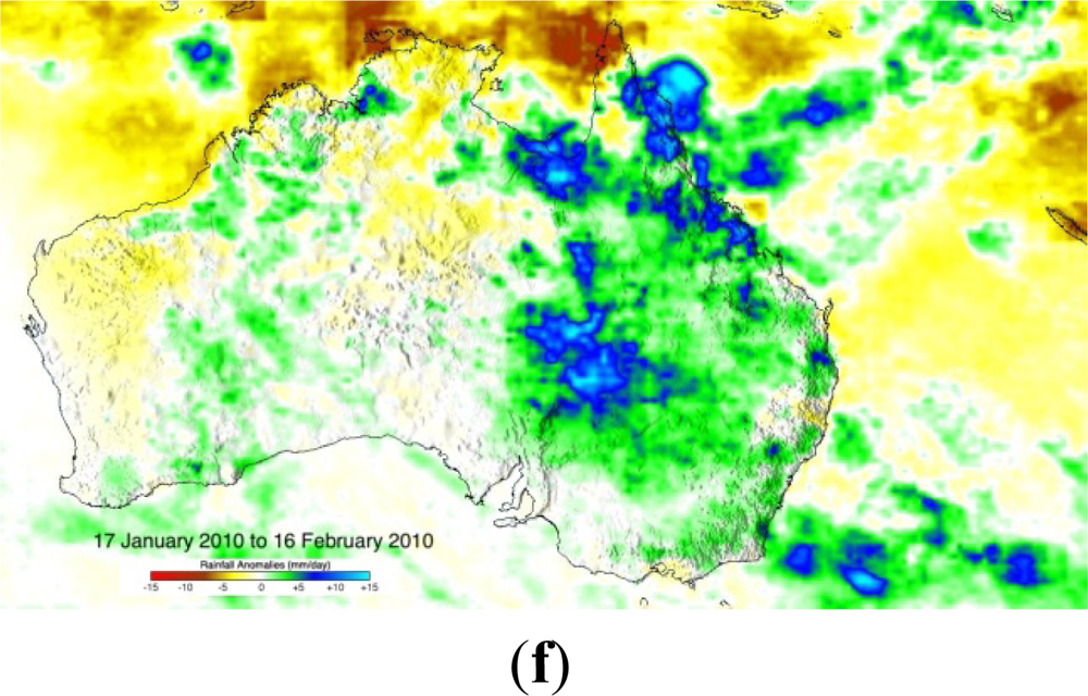
  30. TRMM Mission. Available online: http://trmm.gsfc.nasa.gov/publications_dir/17jan-16feb10_anomaly.html (accessed on 5 March 2012).
  31. Le Vine, D.M.; Haken, M. RFI at L-Band in Synthetic Aperture Radiometers. Proceedings of the 2003 IEEE Geoscience and Remote Sensing Symposium, Toulouse, France, 21–25 July 2003; pp. 1742–1744.
  32. Skou, N.; Misra, S.; Balling, J.; Kristensen, S.; Sobjaerg, S. L-Band RFI as experienced during airborne campaigns in preparation for SMOS. IEEE Trans. Geosci. Remote Sens 2010, 48, 1398–1407. [Google Scholar]
  33. Oliva, R.; Daganzo, E.; Kerr, Y.; Mecklenburg, S.; Nieto, S.; Richaume, P.; Gruhier, C. SMOS RF interference scenario: Status and actions taken to improve the RFI environment in the 1400–1427 MHz passive band. IEEE Trans. Geosci. Remote Sens, 2012; submitted. [Google Scholar]
  34. Camps, A.; Gourrion, J.; Tarongí, J.M.; Gutiérrez, A.; Barbosa, J.; Castro, R. RFI Analysis in SMOS Imagery. Proceedings of the 2010 IEEE International Geoscience and Remote Sensing Symposium, Honolulu, HI, USA, 25–30 July 2010; pp. 2007–2010.
  35. Camps, A.; Vall-llossera, M.; Duffo, N.; Zapata, M.; Corbella, I.; Torres, F.; Barrena, V. Sun effects in 2D aperture synthesis radiometry imaging and their cancellation. IEEE Trans. Geosci. Remote Sens 2004, 42, 1161–1167. [Google Scholar]
  36. Camps, A.; Vall-llossera, M.; Reul, N.; Torres, F.; Duffo, N.; Corbella, I. Impact and Compensation of Diffuse Sun Scattering in 2D Aperture Synthesis Radiometers Imagery. Proceedings of the 2005 IEEE International Geoscience and Remote Sensing Symposium, Seoul, Korea, 25–29 July 2005; pp. 4906–4909.
  37. Martin-Neira, M.; Ribo, S.; Martin-Polegre, J. Polarimetric mode of MIRAS. IEEE Trans. Geosci. Remote Sens 2002, 40, 1755–1768. [Google Scholar]
  38. Camps, A.; Gourrion, J.; Tarongí, J.M.; Vall-llossera, M.; Gutiérrez, A.; Barbosa, J.; Castro, R. Radio-frequency interference detection and mitigation in synthetic aperture radiometers. Algorithms 2011, 4, 155–182. [Google Scholar]
  39. Font, J.; Lagerloef, G.; LeVine, D.; Camps, A.; Zanife, O.Z. The determination of surface salinity with the european SMOS space mission. IEEE Trans. Geosci. Remote Sens 2004, 42, 2196–2205. [Google Scholar]
  40. Camps, A.; Font, J.; Vall-llossera, M.; Corbella, I.; Duffo, N.; Torres, F.; Blanch, S.; Aguasca, A.; Villarino, R.; Gabarró, C.; et al. Determination of the sea surface emissivity at L-band and application to smos salinity retrieval algorithms: Review of the contributions of the UPC-ICM. Radio Sci 2008. [Google Scholar] [CrossRef]
  41. Rautiainen, K.; Kainulainen, J.; Auer, T.; Pihlflyckt, J.; Kettunen, J.; Hallikainen, M. Helsinki university of technology L-band airborne synthetic aperture radiometer. IEEE Trans. Geosci. Remote Sens 2008, 46, 717–726. [Google Scholar]
  42. Camps, A.; Vall.llossera, M.; Batres, L.; Duffo, N.; Torres, F.; Corbella, I. Retrieving sea surface salinity with multi-angular L-band brightness temperatures: Improvement by spatio-temporal averaging. Radio Sci 2005. [Google Scholar] [CrossRef]
  43. Talone, M.; Camps, A.; Sabia, R.; Font, J. Towards a Coherent Sea Surface Salinity Product from SMOS Radiometric Measurements and Argo Buoys. Proceedings of the 2007 IEEE International Geoscience and Remote Sensing, Barcelona, Spain, 23–28 July 2007; pp. 3959–3962.
  44. Talone, M.; Sabia, R.; Camps, A.; Vall-llossera, M.; Gabarró, C.; Font, J. Sea surface salinity retrievals from HUT-2D L-band radiometric measurements. Remote Sens. Environ 2010, 114, 1756–1764. [Google Scholar]
  45. Kainulainen, J.; Colliander, A.; Closa, J.; Martin-Neira, M.; Oliva, R.; Buenadicha, G.; Rubiales, P.; Hakkarainen, A.; Hallikainen, M. Radiometric performance of the SMOS reference radiometers: Assessment after one year of operation. IEEE Trans. Geosci. Remote Sens 2012. submitted.. [Google Scholar]
  46. Tenerelli, J.E.; Reul, N.; Mouche, A.A.; Chapron, B. Earth-viewing L-band radiometer sensing of sea surface scattered celestial sky radiation-Part I: General characteristics. IEEE Trans. Geosci. Remote Sens 2008, 46, 659–674. [Google Scholar]
  47. Reul, N.; Tenerelli, J.E.; Floury, N.; Chapron, B. Earth-viewing L-band radiometer sensing of sea surface scattered celestial sky radiation-Part II: Application to SMOS. IEEE Trans. Geosci. Remote Sens 2008, 46, 675–688. [Google Scholar]
  48. Reul, N.; Tenerelli, J.; Chapron, B.; Waldteufel, P. Modeling sun glitter at L-band for the sea surface salinity remote sensing with SMOS. IEEE Trans. Geosci. Remote Sens 2007, 45, 2073–2087. [Google Scholar]
  49. Anterrieu, E. On the reduction of the reconstruction bias in synthetic aperture imaging radiometry. IEEE Trans. Geosci. Remote Sens 2007, 45, 1084–1093. [Google Scholar]
  50. Klein, L.A.; Swift, C.T. An improved model for the dielectric constant of sea water at microwave frequencies. IEEE Trans. Antennas Propag 1977, 25, 104–111. [Google Scholar]
  51. Ellison, W.; Balana, A.; Delbos, G.; Lamkaouchi, K.; Eymard, L.; Guillou, C.; Prigent, C. New permittivity measurements of seawater. Radio Sci 1998, 33, 639–648. [Google Scholar]
  52. Blanch, S.; Aguasca, A. Seawater dielectric permittivity model from measurements at L-band. Proceedings of the 2004 IEEE International Geoscience and Remote Sensing, Anchorage, AK, USA, 23–28 July 2004; pp. 3959–3962.
  53. Lang, R.; Gu, S.; Jin, Y.; Utku, C.; LeVine, D.M. New Dielectric Model Function for Seawater at L band: Recent Results and Future Plans. Proceedings of the 2010 Aquarius/SAC-D Science Team Meeting, Seattle, WA, USA, 19–21 July, 2010.
  54. Boutin, J.; Waldteufel, P.; Martin, N.; Caudal, G.; Dinnat, E. Surface salinity retrieved from SMOS measurements over the global ocean: Imprecisions due to sea surface roughness and temperature uncertainties. J. Atmos. Ocean. Technol 2004, 21, 1432–1447. [Google Scholar]
  55. Talone, M.; Gourrion, J.; Sabia, R.; Gabarroì, C.; González, V.; Camps, A.; Corbella, I.; Monerris, A.; Font, J. SMOS’ Brightness Temperatures Validation: First Results after the Commisioning Phase. Proceedings of the 2010 IEEE International Geoscience and Remote Sensing Symposium, Honolulu, HI, USA, 25–30 July 2010; pp. 4306–4309.
  56. Meirold-Mautner, I.; Mugerin, C.; Vergely, J.-L.; Spurgeon, P.; Rouffi, F.; Meskini, N. SMOS ocean salinity performance and TB bias correction. Geophy. Res. Abstr 2009, 11. EGU2009–9856.. [Google Scholar]
  57. Tenerelli, J.; Reul, N. Analysis of SMOS Brightness Temperatures Obtained from March through May 2010. Proceedings of the ESA Living Planet Symposium 2010, Bergen, Norway, 28 June–2 July 2010. ESA SP-686..
  58. Talone, M. Contribution to the Soil Moisture and Ocean Salinity (SMOS) Mission Sea Surface Salinity retrieval Algorithm. Ph. D. Thesis, Universitat Politècnica de Catalunya, Barcelona, Spain, 2010; Available online: http://www.tdx.cat/handle/10803/48633 (accessed on 5 March 2012).
  59. Antonov, J.I.; Locarnini, R.A.; Boyer, T.P.; Mishonov, A.V.; Garcia, H.E. World Ocean Atlas 2005, Volume 2: Salinity; Levitus, S., Ed.; NOAA Atlas NESDIS 62; USA Government Printing Office: Washington, DC, USA, 2006; p. 182. [Google Scholar]
  60. Gourrion, J.; Sabia, R.; Portabella, M.; Tenerelli, J.; Guimbard, S.; Camps, A. Characterization of the SMOS instrumental error pattern correction over the ocean. IEEE Geosci. Remote Sens. Lett 2012. [Google Scholar] [CrossRef]
  61. Guimbard, S.; Gourrion, J.; Portabella, M.; Turiel, A.; Gabarró, C.; Font, J. SMOS semi-empirical ocean forward model adjustment. IEEE Trans. Geosci. Remote Sens, 2012; submitted. [Google Scholar]
  62. Torres, F.; Corbella, I.; Duffo, N.; Lin, W.; Gourrion, J.; Font, J.; Martín-Neira, M. Minimization of image distortion in SMOS brightness temperature maps over the ocean. IEEE Geosci. Remote Sens. Lett 2012, 9, 18–22. [Google Scholar]
  63. Srokosz, M.A. Ocean Surface Salinity-the Why, What and Whether. Proceedings of the Consultative Meeting on Soil Moisture and Ocean Salinity Measurement Requirements and Radiometer Techniques (SMOS), Noordwijk, The Netherlands, 20–21 April 1995; pp. 49–56, ESA WPP-87..
  64. Boutin, J.; Martin, N. ARGO upper salinity measurements: Perspectives for L-band radiometers calibration and retrieved sea surface salinity validation. IEEE Geosci. Remote Sens. Lett 2006, 3, 202–206. [Google Scholar]
  65. Salvador, J.; Fernández, P.; Julià, A.; Font, J.; Pelegrí, J.L. A New Buoy for Measurement and Real Time Transmission of Surface Salinity. Proceedings of the 39th CIESM Congress, Venice, Italy, 10–14 May 2010.
  66. de la Fuente, P.; Talone, M.; Marrasé, C.; Romera, C.; Pelegrí, J.L. The Amazon river plume as viewed from remotely sensed and in situ acquisitions. IEEE Trans. Geosci. Remote Sens. (submitted).
  67. Kalman, R.E.; Bucy, R.S. A new approach to linear filtering and prediction problems. Trans. ASME–J. Basic Eng 1960, 82, 35–45. [Google Scholar]
  68. Roullet, G.; Madec, G. Salt conservation, free surface and varying levels: A new formulation for ocean general circulation models. J. Geophy. Res 2000, 105, 23927–23942. [Google Scholar] [CrossRef]
  69. Mourre, B.; Ballabrera-Poy, J.; García-Ladona, E.; Font, J. Surface salinity response to changes in the model parameter and forcings in a climatological simulation of the eastern North-Atlantic Ocean. Ocean Model 2008, 23, 21–32. [Google Scholar]
  70. Mourre, B.; Ballabrera-Poy, J. Salinity model errors induced by wind stress uncertainties in the Macaronesian region. Ocean Model 2009, 29, 213–221. [Google Scholar]
  71. Merlin, O.; Walker, J.P.; Chehbouni, A.; Kerr, Y. Towards deterministic downscaling of SMOS soil moisture using MODIS derived soil evaporative efficiency. Remote Sens. Environ 2008, 112, 3935–3946. [Google Scholar] [Green Version]
  72. Acevo-Herrera, R.; Aguasca, A.; Bosch-Lluis, X.; Camps, A.; Martínez-Fernández, J.; Sánchez-Martín, N.; Pérez-Gutiérrez, C. Design and first results of an uav-borne L-band radiometer for multiple monitoring purposes. Remote Sens 2010, 2, 1662–1679. [Google Scholar]
  73. Carlson, T. An overview of the ‘triangle method’ for estimating surface evapotranspiration and soil moisture from satellite Imagery. Sensors 2007, 7, 1612–1629. [Google Scholar]
  74. Piles, M. Multiscale Soil Moisture Retrievals from Microwave Remote Sensing Observations. Ph. D. Thesis, Universitat Politècnica de Catalunya, Barcelona, Spain, 2010. Available online: http://www.tdx.cat/handle/10803/77910 (accessed on 5 March 2012).
  75. Piles, M.; Camps, A.; Vall-llossera, M.; Corbella, I.; Panciera, R.; Rudiger, C.; Kerr, Y.; Walker, J. Downscaling SMOS-derived soil moisture using MODIS visible/infrared data. IEEE Trans. Geosci. Remote Sens 2011, 49, 3156–3166. [Google Scholar]
  76. Valencia, E.; Camps, A.; Marchan-Hernandez, J.F.; Rodriguez-Alvarez, N.; Ramos-Perez, I.; Bosch-Lluis, X. Experimental determination of the sea correlation time using GNSS-R coherent data. IEEE Geosci. Remote Sens. Lett 2010, 7, 675–679. [Google Scholar]
  77. Valencia, E.; Camps, A.; Bosch-Lluis, X.; Rodríguez-Álvarez, N.; Ramos-Perez, I.; Marchan-Hernandez, J.F.; Eugenio, F.; Marcello, J. On the use of GNSS-R DATA TO Correct L-band brightness temperatures for sea state effects: Results of the ALBATROSS field Experiments. IEEE Trans. Geosci. Remote Sens 2011, 49, 3225–3235. [Google Scholar]
  78. Delwart, S.; Bouzinac, C.; Wursteisen, P.; Berger, M.; Drinkwater, M.; Martín-Neira, M.; Kerr, Y. SMOS validation and COSMOS campaigns. IEEE Trans. Geosci. Remote Sens 2008, 46, 695–704. [Google Scholar]
  79. Valencia, E.; Camps, A.; Rodriguez-Alvarez, N.; Ramos-Perez, I.; Bosch-Lluis, X.; Park, H. Improving the accuracy of sea surface salinity retrieval using GNSS-R data to correct the sea state effect. Radio Sci 2011, 46, RS0C02. [Google Scholar] [CrossRef]
  80. Valencia, E.; Camps, A.; Marchán-Hernandez, J.F.; Bosch-Lluis, X.; Rodríguez-Álvarez, N.; Ramos-Pérez, I. Advanced architectures for real time delay-doppler map GNSS-reflectometers: the GPS reflectometer instrument for PAU (griPAU). Adv. Space Res 2010, 46, 196–207. [Google Scholar]
  81. Nogués, O.; Cardellach, E.; Sanz Campderros, J.; Rius, A.A. GPS-reflections receiver that computes doppler/delay maps in real time. IEEE Trans. Geosci. Remote Sens 2007, 45, 156–174. [Google Scholar]
  82. Camps, A.; Font, J.; Vall-llossera, M.; Gabarró, C.; Corbella, I.; Duffo, N.; Torres, F.; Blanch, S.; Aguasca, A.; Villarino, R.; et al. The WISE 2000 and 2001 field experiments in support of the SMOS mission: Sea surface L-band brightness temperature observations and their application to multi-angular salinity retrieval. IEEE Trans. Geosci. Remote Sens 2004, 42, 804–823. [Google Scholar]
  83. Rodriguez-Alvarez, N.; Camps, A.; Vall-llossera, M.; Bosch-Lluis, X.; Monerris, A.; Ramos-Perez, I.; Valencia, E.; Marchan-Hernandez, J.F. Land geophysical parameters retrieval using the interference pattern GNSS-R technique. IEEE Trans. Geosci. Remote Sens 2011, 49, 71–84. [Google Scholar]
  84. Valencia, E.; Camps, A.; Vall-llossera, M.; Monerris, A.; Bosch-Lluis, X.; Rodriguez-Alvarez, N.; Ramos-Perez, I.; Marchan-Hernandez, J.F.; Martinez-Fernandez, J.; Sanchez-Martin, N.; et al. GNSS-R Delay-Doppler Maps over Land: Preliminary Results of the GRAJO Field Experiment. Proceedings of the 2010 IEEE International Geoscience and Remote Sensing Symposium, Honolulu, HI, USA, 25–30 July 2010; pp. 3805–3808.
  85. Delta-T Devices. Available online: http://www.delta-t.co.uk/product-display.asp?id=ML2x%20Product&div=Soil%20Science (accessed on 5 March 2011).
  86. Spurgeon, P.; Font, J.; Boutin, J.; Reul, N.; Tenerelli, J.; Vergely, J.L.; Gabaro, C.; Yin, X.; Lavender, S.; Chuprin, A.; et al. Ocean Salinity Retrieval Approaches for the SMOS Satellite. Proceedings of the ESA Living Planet Symposium, Bergen, Norway, June 28–July 2 2010. ESA Special Publication SP-686..
Figure 1. (a) PMS offset jumps correlated with heater signals; (b) Correction implemented to estimate the offset from its mean value, the physical temperature and the heater signals; (c) PMS gain [mV/K] drifts: observations along the orbit (green), estimated from on-ground measurements (blue), and from in-flight measurements (red); (d) Local oscillator phase drifts estimated from noise injection calibration and tracking using spline interpolation (from [21]).
Remotesensing 04 01272f1
Figure 2. Radiometric Sensitivity over Ocean at (a) X-polarization and (b) Y-polarization in the antenna reference frame; and (c) cut at = 0: comparison with the theoretical model (dashed lines) [26,27]. Note that at ξ = 0, X- and Y-polarizations are equal to H- and V-polarizations (from [21]).
Remotesensing 04 01272f2
Figure 3. Images from [21]: (a) Amazon river plume as seen from Soil Moisture and Ocean Salinity (SMOS) on 5–9 May 2010 (left) and 14–19 May 2010 (right); (b) Imaging of Antarctica, blue cross indicates location of Concordia Station in the Dome-C area; and (c) inter-comparison between one SMOS overpass data (dots) and DOMEX 2004-derived antenna temperatures (solid lines) [10]. Australia imaged (d) before and (e) after passage of hurricane Olga. Note the lower antenna temperatures associated to higher soil moisture values. Note: All images represent (TH+TV)/2 on the alias-free field of view (FOV) for all incidence angles; (f) Rainfall anomalies measured by TRMM from 17 January 2010 to 16 February 2010 (from [30]).
Remotesensing 04 01272f3aRemotesensing 04 01272f3b
Figure 4. (a) Original X-polarization brightness temperature corrupted by RFI; (b) brightness temperature cleaned from RFI; (c) RFI image subtracted from 4(a) to obtain 4(b): RFI is clearly seen as a hot spot in the middle of the island; and (d) confidence level of the RFI sources subtracted. (Figure 4(a,b) from [38]).
Remotesensing 04 01272f4
Figure 5. (a) Eight cells considered in the study superimposed onto the Helsinki University of Technology (HUT) sample location; the surface salinity measured by the vessel and interpolated to the salinity retrieval grid is shown in the figure; white stars are for the vessel measurement locations; (b) Sea surface salinity retrievals in different configurations. Red: no bias correction. Positive brightness temperature biases tend to underestimate the retrieved salinity values, so it saturates at 0 psu. Blue: estimated instrumental constant bias subtracted to measured brightness temperatures, leads to overestimation of the retrieved salinity values by 7–13 psu. Green: external brightness temperature calibration applied reduces the biases, although a positive bias still exists. Vessel measurements in black for comparison; (c) Retrieved salinity after averaging (solid line) vs. the measured salinity (from [44]).
Remotesensing 04 01272f5
Figure 6. (a) WOA05 climatology (scale from 30 to 45 psu); (b) Level 3 ten-day map minus WOA05 climatology for the nominal case—no bias mitigation applied; (c) external brightness temperature calibration applied; and (d) model-dependent ocean target transformation applied (model 2 dual polarization obtained from full-polarimetric data, third and fourth Stokes parameters neglected) (from [58]).
Remotesensing 04 01272f6
Figure 7. Evolution of the averaged rms of the Ocean Target Transformation (OTT) mismatches as a function of the number of days following the FTR calibration, for both TX and TY, and the First Stokes parameter divided by two. Dashed lines correspond to the averaged standard deviation. (Figure 3 from [60]).
Remotesensing 04 01272f7
Figure 8. Surface drifter for near surface salinity measurements with real-time or near real-time transmission capabilities designed and deployed for SMOS validation [65].
Remotesensing 04 01272f8
Figure 9. (a) Track of the Hespérides research vessel; (b) SMOS-derived sea surface salinity using Model 2; and (c) sea surface salinity anomalies measured from the Hespérides (dark blue), and the three outputs from the SMOS L2 ocean salinity processor (red: SSS 1, two-scale model; green SSS2, SSA model; and light blue SSS3 semi-empirical model) (from [66]).
Remotesensing 04 01272f9aRemotesensing 04 01272f9b
Figure 10. (a) Instantaneous sea surface salinity of the regional model simulation; and (b) model SSS response to forcing and parameters changes. The four open boundary conditions are oriented South-North (15°N and 44°N) and East-West. (45°W and the Gibraltar Straight). Relative surface salinity response of forcing parameters (“τ” wind stress, “W”wind speed, “H” atmospheric humidity and “T” temperature, “P” precipitation, and “O” the data controlling the boundary condition) and models parameters and model parameterization (“V” changing from bi-Laplacian horizontal viscosity to a Laplacian one, “L” changing the Laplacian diffusion coefficient of salinity; “M” changing the vertical mixing scheme; switching-off double diffusion parameterization -“D”- and river-runoff -“R”-; switching-on the Newtonian relaxation of SST -“τi”- and SSS -“τs”- towards their climatic values), (adapted from [70]).
Remotesensing 04 01272f10
Figure 11. Location of the REMEDHUS calibration and validation site in the central part of the Duero basin, Spain Layout of the 23 permanent soil moisture stations within REMEDHUS soil moisture measurement network.
Remotesensing 04 01272f11
Figure 12. UPC Airborne Radiometer at L-band (ARIEL) retrieved TB [K] obtained at heights 140 ± 30 m (spatial resolution ∼50 m), re-sampled to a 60 × 60 m grid and geo-referenced on Google Earth (from [74]).
Remotesensing 04 01272f12
Figure 13. Scatter plot of LANDSAT Ts vs. LANDSAT NDVI of the area corresponding to Flight 1. The triangle concept is used to link this LANDSAT NDVI/Ts space to airborne soil moisture (from [74]).
Remotesensing 04 01272f13
Figure 14. Ground-based soil moisture (left column), ARIEL-derived soil moisture (second column), down-scaled soil moisture (third column), and associated errors (fourth and fifth columns, computed as first column minus the second, and the first column minus the third one, respectively). Upper row: Flight 1; lower row: Flight 2 (from [74]).
Remotesensing 04 01272f14
Figure 15. (a) Murrumbidgee catchment elevation and permanent soil moisture monitoring network; (b) Layout of permanent and semi-permanent SM stations within Yanco intensive monitoring region; (c) Surface soil moisture (sm) and daily rainfall in the different rain gauges of the network (from [75]).
Remotesensing 04 01272f15
Figure 16. Sample results with SMOS data over the Murrumbidgee catchment, from 17 February 2010 (6 am). (a) SMOS soil moisture [m3/m3] on a 40 × 40 grid; (b) 1 km SMOS-derived soil moisture maps [m3/m3] using the linking model in (2); (c) 1 km SMOS-derived soil moisture maps [m3/m3] using the linking model in (3); (d) SMOS TBh image [K] at 42.5° on a 40 × 40 km grid; (e) 1 km MODIS/TERRA Ts [K]; (f) 1 km MODIS/TERRA NDVI. Empty areas in the image correspond to unsuccessful SMOS soil moisture retrievals, or clouds masking MODIS Ts measurements.
Remotesensing 04 01272f16
Figure 17. Sample results with SMOS data over the Iberian Peninsula, from 22 August 2011 (6 pm). (a) SMOS soil moisture [m3/m3] on a 40 × 40 grid; (b) 1 km SMOS-derived soil moisture maps [m3/m3] using the linking model in (3); (c) SMOS TBh image [K] at 42.5° on a 40 × 40 km grid; (d) 1 km MODIS/TERRA Ts [K]; (e) 1 km MODIS/TERRA NDVI. Empty areas in the image correspond to unsuccessful SMOS soil moisture retrievals, or clouds masking MODIS Ts measurements.
Remotesensing 04 01272f17
Figure 18. Measured (not normalized, in arbitrary units) one second incoherently averaged Delay-Doppler Map (DDM) with the threshold applied to compute the volume contained by it. Noise is well below the threshold (from [77]).
Remotesensing 04 01272f18
Figure 19. (a) griPAU instrument deployed in a 380 m cliff in the North coast of Gran Canaria; (b) Estimated brightness temperature sensitivity to changes in the normalized DDM volume at vertical (red) and horizontal (blue) polarizations respectively. Values at H-pol and θi = 65° and 70° are probably erroneous due to reflections in the cliff (from [77]).
Remotesensing 04 01272f19
Figure 20. (a) Instantaneous variations of the first Stokes parameter (TUD’s EMIRAD nadir looking antenna) and area under the normalized waveform (same philosophy as explained for the DDM volume, but in the experiment IEEC’s GOLD-RTR did not compute DDMs); (b) Retrieved sea surface salinity values using GNSS-R data. Data from COSMOS-OS field experiment generously provided by ESA (from [79]).
Remotesensing 04 01272f20
Figure 21. Microwave remote sensors deployed at the GRAJO 2008–2010 field experiment site.
Remotesensing 04 01272f21
Figure 22. Geolocated (a) peak of the DDM during a satellite pass; and (b) points of the in situ measured soil moisture map; (c) Scatter plot between the in situ soil moisture values and the peak of the DDM showing a strong correlation (r = 0.83). The trend is linear indicating that the peak of the DDM is proportional to the soil’s reflectivity, which is related to the soil moisture content (from [84]).
Remotesensing 04 01272f22

