Application of Semi-Automated Filter to Improve Waveform Lidar Sub-Canopy Elevation Model
by

Geoffrey A. Fricker
1,*, 
Sassan S. Saatchi
2,
Victoria Meyer
2,
Thomas W. Gillespie
1 and
Yongwei Sheng
1 1
Department of Geography, University of California, Los Angeles. 1255 Bunche Hall Box 951524, Los Angeles, CA 90095, USA
2
Jet Propulsion Laboratory, California Institute of Technology. 4800 Oak Grove Drive, Pasadena, CA 91109, USA
*
Author to whom correspondence should be addressed.
Remote Sens. 2012, 4(6), 1494-1518; https://doi.org/10.3390/rs4061494
Submission received: 21 March 2012
/
Revised: 11 May 2012
/
Accepted: 14 May 2012
/
Published: 25 May 2012
(This article belongs to the Special Issue Laser Scanning in Forests)
Abstract
:Modeling sub-canopy elevation is an important step in the processing of waveform lidar data to measure three dimensional forest structure. Here, we present a methodology based on high resolution discrete-return lidar (DRL) to correct the ground elevation derived from large-footprint Laser Vegetation Imaging Sensor (LVIS) and to improve measurement of forest structure. We use data acquired over Barro Colorado Island, Panama by LVIS large-footprint lidar (LFL) in 1998 and DRL in 2009. The study found an average vertical difference of 28.7 cm between 98,040 LVIS last-return points and the discrete-return lidar ground surface across the island. The majority (82.3%) of all LVIS points matched discrete return elevations to 2 m or less. Using a multi-step process, the LVIS last-return data is filtered using an iterative approach, expanding window filter to identify outlier points which are not part of the ground surface, as well as applying vertical corrections based on terrain slope within the individual LVIS footprints. The results of the experiment demonstrate that LFL ground surfaces can be effectively filtered using methods adapted from discrete-return lidar point filtering, reducing the average vertical error by 15 cm and reducing the variance in LVIS last-return data by 70 cm. The filters also reduced the largest vertical estimations caused by sensor saturation in the upper reaches of the forest canopy by 14.35 m, which improve forest canopy structure measurement by increasing accuracy in the sub-canopy digital elevation model.
1. Introduction
Light Detection and Ranging (LiDAR) is a widely used active remote sensing method used to produce high accuracy 3-dimensional models of forest structure and sub-canopy topography in forested areas. For ground mapping applications, generally high density discrete-return lidar (DRL) is used to accurately map sub-canopy topography. To map large heavily forested areas, improved methods are necessary which improve the ground detection accuracy of large-footprint lidar (LFL) for the next generation of high-altitude airborne and spaceborne lidar sensors. Active remote sensing is particularly sensitive to changes in biomass in recently disturbed forest or secondary growth forest. However, most active remote sensing systems have saturation problems in areas of high biomass forests [1,2]. Tall multi-layered vertically stratified forest canopy conditions can occlude the lidar signal and produce errors in the sub-canopy digital elevation model (DEM). This problem is particularly problematic using LFL in variable topography. We test new methods for improving sub-canopy DEM accuracy using LFL in a densely vegetated Neotropical rainforest.
Lidar sensors are the best technique for assessing tropical forest structure and biomass at local to sub-national scales [3,4]. Lidar can accurately measure the forest’s vertical structure, making possible estimates of aboveground biomass, habitat structure and topography [5]. In forests, lidar sensors use the return signals to detect the height of the canopy top, ground elevation and the positions of leaves and branches [6]. For the purpose of this study, the two types of airborne lidar remote sensing being used are DRL and LFL, also commonly referred to as waveform lidar. The Laser Vegetation Imaging Sensor (LVIS) is an experimental version of LFL developed by NASA to fly at high altitudes (>1 km) and meant as a validation sensor for the Vegetation Canopy Lidar mission [7]. LFL and LVIS can be used interchangeably in our study. However, the methods presented are meant for any LFL survey including spaceborne lidar, with sufficient point density and should not be restricted to LVIS. Although laser altimetry can provide both the sub-canopy topography as well as vertical canopy structure, significant differences between DRL and LFL exist and should be emphasized. DRL lidar footprints are generally very small (<50 cm), while LFL such as LVIS generally have footprint sizes larger than 15 m [7]. In the case of a DRL survey, the ground surface within an average DRL footprint can be considered a planar surface [8]. Under most operating circumstances airborne LFL footprints are around 20–25 m in diameter and the ground surface can include considerable topographic variation, which dramatically affects the last-return’s waveform shape [7].
Large-footprint lidar was first tested on a spaceborne platform as the Geoscience Laser Altimeter System (GLAS), which was the sole instrument on board the Ice, Cloud and land Elevation Satellite (ICESat). The primary mission of ICESat was to measure the polar ice-sheets; however it was also used extensively to measure global vegetation height and forest structure [9–11]. One of the largest sources of inaccuracy in GLAS measurements was the impact of terrain slope and micro-topography within the GLAS footprint, which average approximately 70 m in diameter [12]. In steep terrain, the trailing edge of a waveform can be elongated, stretching the last return over a vertical distance. Lefsky et al. showed that topography in a footprint could be directly calculated from the shape of the last-peak of the lidar waveforms trailing edge and developed a systematic method to correct GLAS waveforms for the effects of topography [13]. Spaceborne LFL is attractive to scientists and policy makers because of its ability to measure forest biomass at the global scale. ICESat 2 is currently being planned for launch in early 2016, and next generation spaceborne lidar systems will have smaller footprint size and increased density of measurements on the ground [14,15].
Airborne DRL is a highly accurate and spatially explicit altimetry method, due to low collection altitudes and repeated passes which can collect multiple laser measurements per square meter (ppm2). As DRL laser pulses travel through the canopy multiple laser returns or ‘echoes’ often occur, which results in additional discrete point measurements of canopy structure per laser pulse. The high spatial resolution allows DRL to measure individual leaves and branches in the canopy profile, which requires low-altitude (500 m–1,500 m) airborne operation and results in a narrow mapping swath width. Consequently mapping large areas requires extensive flying [16]. Airborne DRL has been used in numerous studies in dense tropical forests and has proven effective in accurately estimating biomass, determining sub-canopy topography and forest structure [17–19].
Airborne LVIS LFL can provide a more cost effective alternative to airborne DRL due to higher collection altitudes and subsequently wider mapping swaths on the ground. LFL is especially well suited for mapping forest ecosystems due to expanded spatial coverage and a large footprint size, which generally exceeds the average crown diameter of large emergent trees in closed canopy forests [20,21] and thereby allows laser energy to reach the ground through inter-crown gaps [22]. However, over topographically complex terrains, LFL waveforms may suffer from beam-broadening and slope effects that can introduce errors in estimating surface elevation. One of the largest sources of uncertainty in estimating forest height and vertical structure using both DRL and LFL is accurately determining the sub-canopy topography under dense vegetation [23]. Producing accurate sub-canopy DEMs is a high priority for lidar and other sensors designed for mapping structure such as Synthetic Aperture Radar (SAR). Any improvements in sub-canopy topography have a considerable effect on forest structure and biomass estimation [16]. Using DRL data acquired at less than 1 m footprint will allow us to examine the errors in LFL data and correct the surface elevation and derived forest structure.
Techniques for DRL point filtering to improve DEM quality have been well explored by both the academic and private sectors [24–27]. However, to our knowledge, LFL point filtering has not yet been rigorously examined as a method to improve the sub-canopy DEM and associated forest canopy measurements. Once the correction is developed over study areas where both DRL and LFL are acquired, the methodology can be implemented on LFL data collected in other regions. LFL can potentially cover larger regions compared to low-altitude DRL surveys and has proven effective in producing accurate estimations of sub-canopy topography, vertical canopy structure and biomass [28–30]. While the LVIS team has made all reasonable efforts to remove questionable data, errors are still present [7]. This paper proposes a semi-automated method for filtering LFL data to improve DEM quality and increase the accuracy of the resulting waveform data which relates directly to forest structure. The proposed methodology will use only the LFL sub-canopy DEM to estimate slope, to improve the LFL post-processing methods to account for large errors in ground elevation through filtering and to understand and correct for the effects of terrain slope on sub-canopy topography, in the absence of a DRL DEM.
Barro Colorado Island (BCI), Panama has variable topography and dense canopy vegetation which provide an ideal environment to test the canopy penetration capabilities of lidar sensors and the effects of sub-canopy topography. We focus on the 50-ha forest dynamics plot on BCI because it has been surveyed using conventional methods and is composed of mostly old-growth forest containing some of the largest trees on the island. It also encompasses the edge of a plateau at the southern edge of the plot where terrain steepness increases. This contiguous condition of steep terrain connected to surveyed old growth forest ideally suits our study of sub-canopy topography. The 50-ha plot also provides spatially accurate structural information and species composition data, which will be the focus of future research. The majority of forest biomass is contained in the largest trees and these are also the specific areas in which sensors are likely to saturate and underestimate biomass and overestimate sub-canopy topography [31,32].
2. Materials and Methods
2.1. Study Area and Field Data
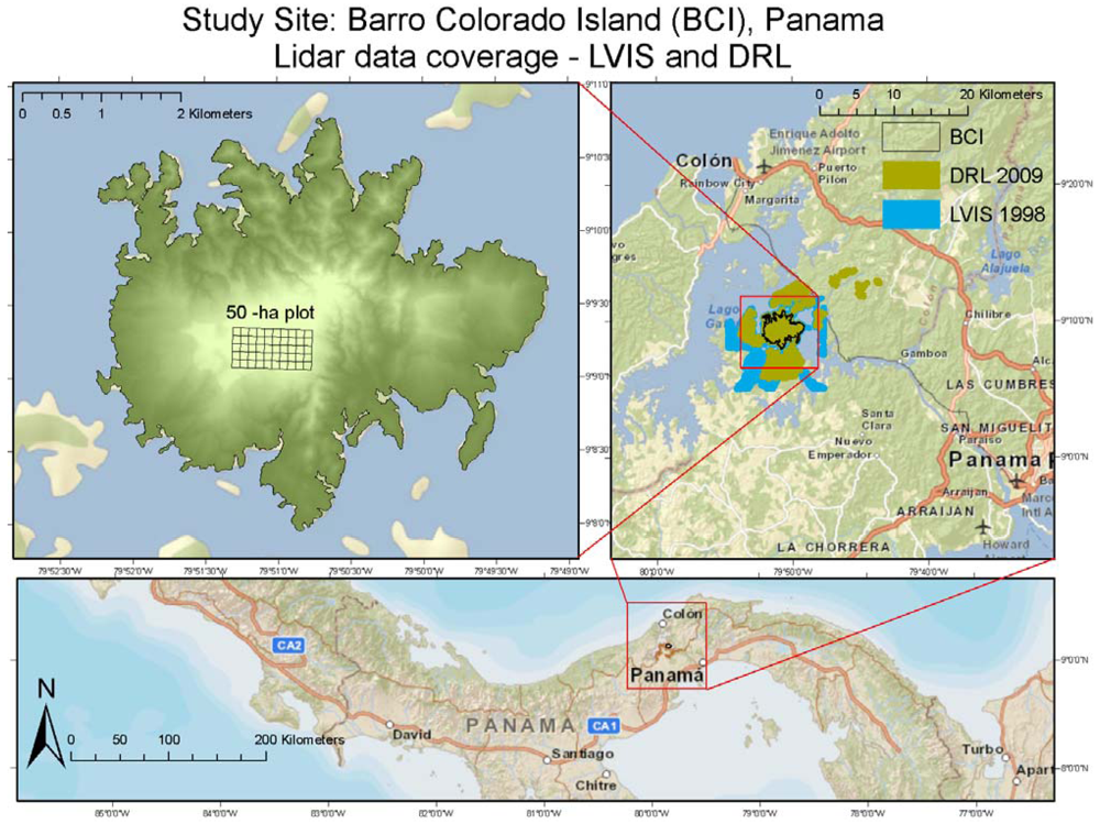
This study was conducted in the moist lowland tropical forest on Barro Colorado Island (BCI), a 15.6 km2 island in the Gatun Lake located in the middle of the Panama Canal Zone watershed in central Panama (Figure 1). BCI is a research reserve for the Smithsonian Tropical Research Institute and is covered in tropical moist forest that receives approximately 2,637 mm of annual precipitation. It has a four-month dry season between January and April when 10% of the canopy species lose their leaves [33]. In 1980, the Forest Dynamics Plot (FDP), a 50-ha vegetation plot was established in a relatively uniform area of BCI’s tropical moist forest with relatively low elevation variation within the plot [34]. The plot is located at the top of the main plateau on BCI, although most of the plot is flat (<10 degrees), the edge of the plateau is in the south-eastern part of the plot and some slopes exceed 30–40 degrees.
In the BCI 50-ha plot, topography was surveyed every 20 m using conventional methods and in a finer scale where topography changed sharply (i.e., in the stream gullies) [35]. Using the kriging estimation method to interpolate between survey measurements, field elevation data is provided at 5 m intervals, resulting in 20,000 separate local ground elevation measurements within the plot. The surveyed plot data were used in the analysis to check the relative accuracy of the DRL DEM. In July 2008, 86 ground elevations were measured using radio-corrected GPS in and around the 50-ha plot. The GPS signal is significantly degraded by overhead canopy and points were collected in tree fall gaps where a minimum number of satellites could be viewed by the GPS receiver. The GPS signal was corrected using the nearby GPS radio-correction beacons used by the Canal Authority. The GPS control points were collected only when GPS satellite coverage yielded vertical error of less than ±1 m in vertical accuracy. GPS control points were not distributed evenly throughout the plot or island due to heavy canopy closure and lack of reliable GPS signal. The most accurate field control points available for our study are 36 Differential Global Positioning System (DGPS) survey points which were collected in 2009 to ensure the relative and absolute accuracy of the DRM DEM.
2.2. Lidar Data
DRL data were collected over BCI during the wet season in 10 days and 11 separate flights in 2009 by Blom Corporation and Northrop Grumman for a joint NASA/JPL and NSF project between 15 August and 10 September. The data were collected using fixed wing aircraft with an Optech 3100 scanning at a rate of 70 KHz. The data yielded a total of over 233 million laser shots and over 528 million individual points, resulting in a point density of 5.6 points per square meter (ppm2) and 8.1 returns per square meter (rpm2). The DRL data was post-processed by Blom Corporation using Bentley’s MicroStation to calibrate and filter the data. In addition to the automated filtering process, additional manual editing of the sub-canopy DEM was performed to produce a bare-earth DEM product. For the purpose of this study, this bare-earth DEM is considered to be actual ground surface, against which the LFL last-pulse elevations are tested. Previous studies have found that DRL is capable of creating accurate DEMs even under dense tropical vegetation using inverse distance weighted and ordinary kriging geostatistical techniques to estimate sub-canopy topography. A study by Clark et al. found a linear correlation of 1.00 m and a Root Mean Squared Error (RMSE) of 2.29 m when compared with 3,859 well-distributed ground survey points at the La Selva Biological Station in Costa Rica [17].
LVIS is an airborne scanning laser altimeter designed and developed at NASA’s Goddard Space Flight Center to be the airborne simulator for the Vegetation Canopy Lidar mission. LVIS design goals include: wide swath, high-altitude capability, variable sampling pattern and footprint diameter, outgoing and return pulse digitization, accurate ranging and automated real-time ground finding/tracking [7]. LVIS is a waveform digitizing sensor which records the entire time-varying amplitude of the backscattered energy in 30-cm vertical bins. This waveform or profile is related to the vertical distribution of intercepted surfaces from the top of the canopy to the ground. The incident laser pulse interacts with canopy and ground features and is reflected back to the telescope of the instrument. LVIS has demonstrated its ability to determine surface topography (including sub-canopy) as well as vegetation height and structure in old growth tropical rainforest [28,30]. The system is capable of operating up to 10 km AGL, generating a 1,000 m wide swath of data using a nominal footprint size of 25 m.
LVIS LFL waveform data were collected by NASA over BCI during the dry season on 29 March 1998 [7,16]. In LVIS post-processing, the LVIS waveforms are analyzed for the last-pulse, as well as percentile metrics, which correspond to the level of total light energy reflected throughout the vertical profile of the laser pulse as it travels through the canopy. The percent of total waveform energy under the waveform curve is referenced to the last-pulse elevation (Zg) to produce relative height (rh) quartiles [36], rh25, rh50, rh75 and rh100 (canopy top). For this study, only the last-return LVIS Zg elevations were used. The 1998 Panama LVIS survey, which was flown at approximately 1 km above ground level, consisted of 215,984 individual LVIS laser shots. 98,040 of the LVIS shots are located over BCI and used for the study. Each LVIS footprint was approximately 20–25 m in diameter depending on scan angle and topography. We chose to focus solely on the ground data due to the inevitable change in forest structure occurring in the nearly 10 years between lidar collections, as well as differences in the phenological and physical characteristics of the forest canopy between wet/dry seasons [21,37].
2.3. Methodology
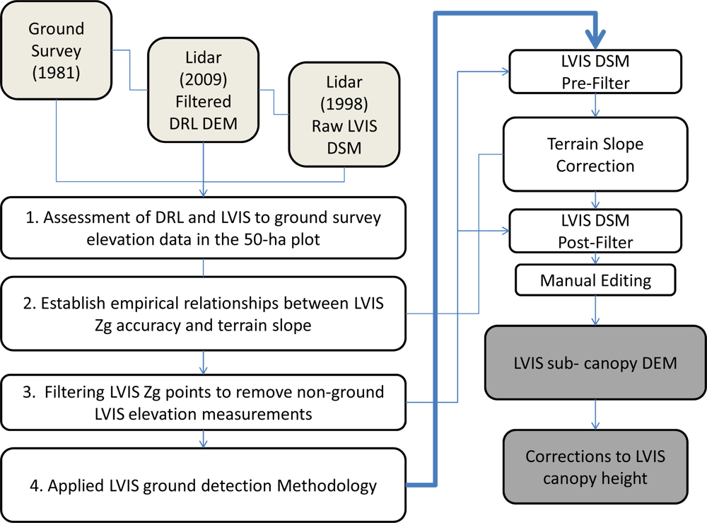
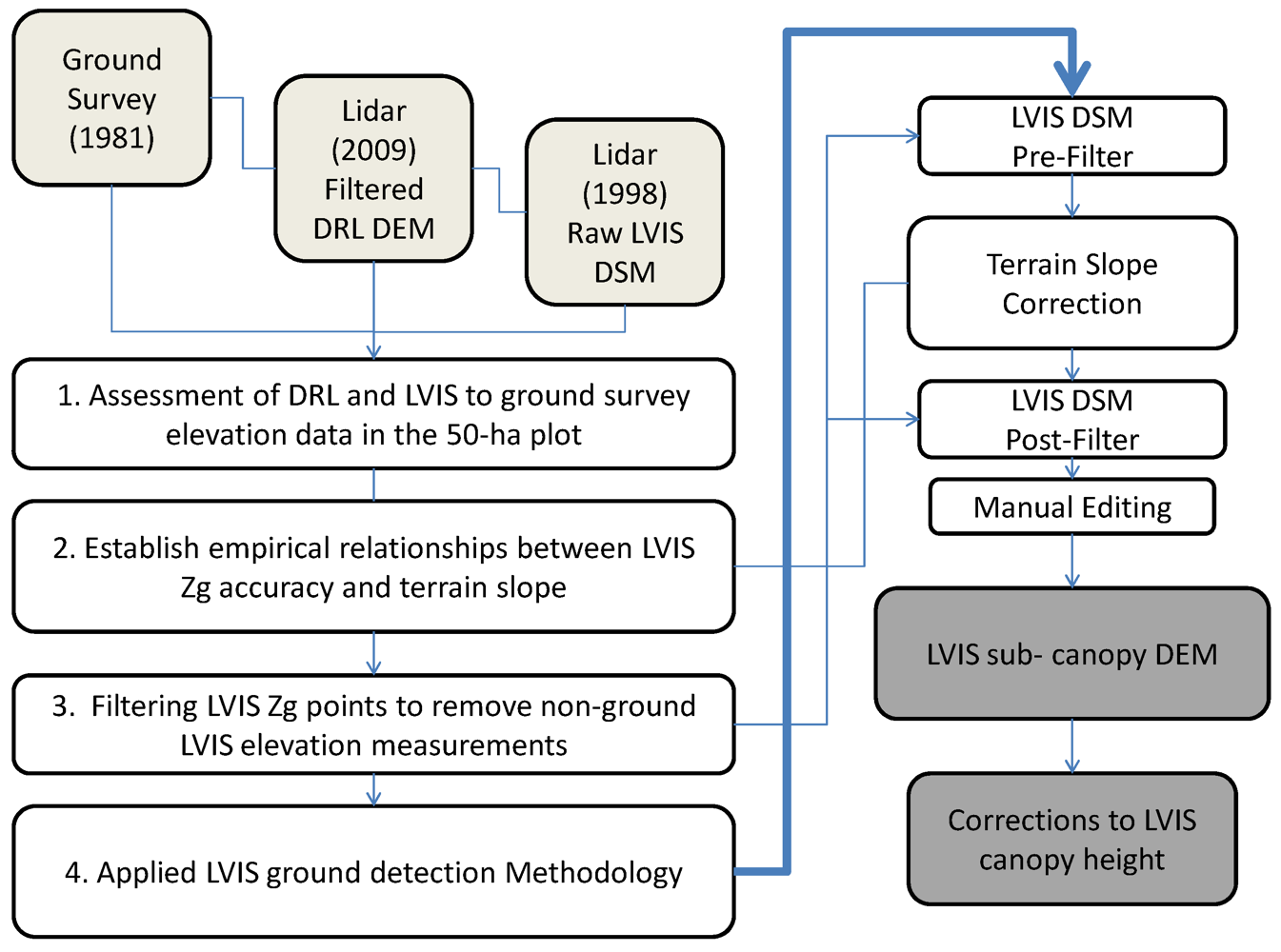
We introduce a new LFL processing methodology based on the comparison of LFL and DRL to improve the sub-canopy DEM derived from LFL Zg last-return data. First, we assess the accuracy of the DRL DEM and LFL Zg digital-surface model (DSM) compared to the 50-ha plot ground survey elevation data. We also test the DRL DEM against Differential GPS (DGPS) and radio-corrected GPS control points. When we refer to the DSM, we imply that it is the unfiltered, unadjusted LVIS Zg surface model. Once processing occurs, non-ground points are removed from the sub-canopy DSM and we refer to it as a DEM, which implies some level of post-processing and an improvement on the original LVIS DSM. Secondly, we analyze the relationship between terrain slope and LFL Zg accuracy to establish empirical relationships which will be used to correct LFL Zg elevations. Third, we analyze topographic anomalies in the LFL DSM and create LFL Zg filters which are capable of removing some of the extreme outliers from the LFL sub-canopy DEM. Lastly, we test a new applied LFL processing methodology which applies both filtering and slope correction methods to create an improved LFL DEM. The new methodology has four distinct steps to improve LFL ground detection, which draw from the initial analysis (Figure 2). The first is to pre-filer the LFL DSM to remove all extreme outliers and generate a preliminary DEM, the second uses the preliminary DEM to apply vertical corrections based on approximate slope to the original LFL Zg points. The third is to re-apply the filters to the slope adjusted LFL Zg points to produce a filtered and slope corrected DEM. The final step is a manual editing process to remove LFL Zg values which were not removed by the filters but appear visually anomalous. The end result is an improved LFL DEM and associated corrections to LFL canopy heights. The approach is designed to be applied over regions where DRL data is not available.
2.3.1. Assessment of DRL and LVIS to Ground Survey Elevations in the 50-ha Plot
To verify the accuracy of the DRL DEM, we tested the vertical differences between the survey data within the 50-ha plot and GPS control points. To quantify absolute elevation accuracy and compliance with the DRL survey precision requirements, the ground surface was independently verified using 36 ground surveyed points on flat, hard, well defined surfaces, free of obstacles which occlude GPS signal. Elevation data from the 1981 field survey of the 50-ha plot were used to create a grid of 20,000 elevation measurements at 5 m spacing. These elevations were not originally referenced to the GPS ellipsoid (WGS84) and were therefore used to check the relative accuracy and not the absolute accuracy of the DRL DEM. A third set of radio-corrected GPS control points were also used to test the DRL DEM under canopy cover.
After the verification of the DRL DEM, we perform the statistical assessment of LFL Zg elevation and the associated DRL bare-earth DEM. By viewing both DRL and LFL points simultaneously, the DRL control surface can be used to determine the best possible estimate of LFL accuracy under dense tropical vegetation. In this section, the DRL DEM is the Triangulated Irregular Network (TIN) bare-earth surface created from filtered and manually edited DRL last-return data. For the purpose of our study, it is considered the true surface DEM. The difference between the control DRL DEM surface and LFL DSM provide an assessment of the canopy penetration capabilities of LFL (Figure 2). The vertical differences between the LFL Zg elevation and the DRL DEM are determined by using the ‘run control report’ function in Terrascan. This function is generally used to calculate vertical accuracy of DRL DEMs from ground based control points. The LFL Zg elevation is compared to the TIN surface created by the three nearest DRL points, using three specific parameters. The maximum size of the triangle is the first parameter, which was set at 20 m, the maximum slope allowed in the triangle was set to 90 degrees and the third parameter z-tolerance was not used due to the large triangle size. The control report output calculates the vertical difference by subtracting the LFL Zg elevation from the elevation of the TIN surface of the three nearest neighbors of the DRL DEM. All results will be presented in this manner, with vertical differences being DRL TIN surface minus the center of the LFL footprint. Negative values indicate an LFL point which is above the ground surface and positive values indicate a LFL Zg elevation below the DRL DEM surface.
2.3.2. Establishing Empirical Relationships between LFL Zg Accuracy and Terrain Slope and Applying Slope Dependent Elevation Adjustments
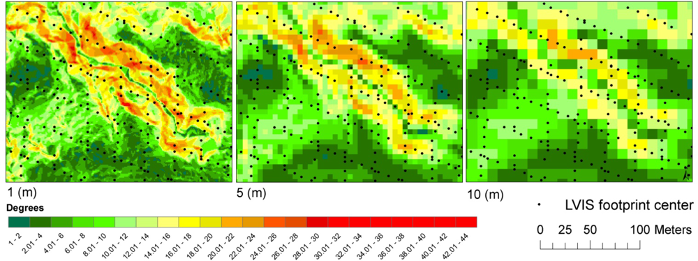
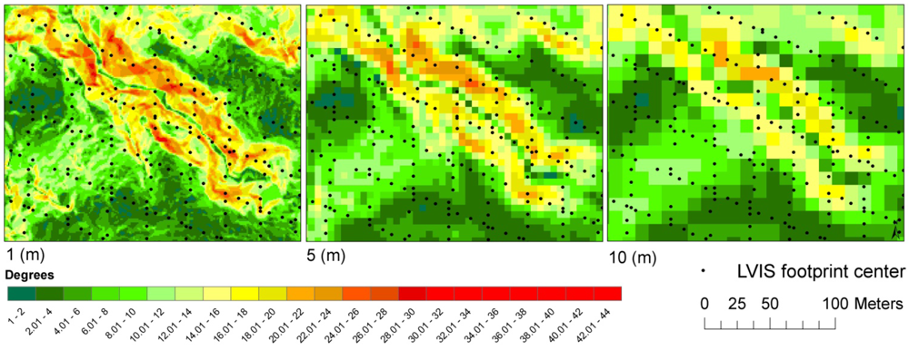
To quantify and model the effects of terrain slope on LFL Zg accuracy, the DRL derived DEM was used as a control surface to determine the terrain slope at the center of each LFL footprint. The DRL derived DEM was output in Terrascan from the filtered DRL bare earth TIN at three (1, 5 and 10 m) spatial resolutions and was used as the control surface to test LFL Zg elevation measurements. Using 3D analyst in ArcGIS 9.3, we created three terrain slope maps derived from the DRL DEM at the same spatial resolutions (Figure 4). These three separate spatial resolutions were used to determine if changes in spatial scale had an impact on the LFL correction. Different spatial resolutions were chosen to ensure a smaller slope pixel size than the LFL footprint and to simulate different DRL ground point densities, which can be sparse in areas of heavy vegetation. As the spatial resolution becomes increasingly coarse, the maximum slope within the LFL footprint decreases from 68, to 66, to 48 degrees, respectively at 1, 5 and 10 m pixel resolutions. The coarser the spatial resolution of the DEM image data, the fewer small terrain features are captured and the flatter the overall topography appears. It is important to use fine resolution slope data, in order to effectively measure small changes in terrain topography, which are effectively lost at larger footprints of LVIS.
The LFL laser energy is Gaussian in nature and focused at the center of laser footprint which is approximately 20–25 m in diameter, depending on terrain and laser incidence angle. The DRL DEM was used to determine the terrain slope in the center of each LFL footprint. To quantify the differences in slope, the slope image was classified into small (2 degree) bins and then converted to polygons, each with its own terrain slope class. The DRL-derived slope class polygons were used to sort LFL Zg points into separate slope classes and tested independently of each other. BCI has areas of steep terrain, including areas at the southern edge of the 50-ha plot on a plateau in the middle of the island, as well as numerous stream channels and gullies. However, LFL shots in high (+45°) slope areas were very rare on BCI (only 0.01% of the total LVIS shots) and were not used for this analysis. The average, maximum/minimum errors, the standard deviation, average magnitude (average absolute value) and root mean squared (RMS) where all calculated for the LFL points in each 2 degree slope class.
To remove the slope dependent biases from the LFL Zg elevations, the 10 m DRL DEM was used to match the spatial scale coincident with the center of the LVIS footprint. For each slope class determined by the slope map, the average difference between LFL Zg elevation and the DRL DEM was the value which was subtracted. Vertical adjustments of less than a meter were applied to slopes less than 30 degrees. However in terrain slopes of greater than 30 degree, progressively larger vertical biases were removed. In the instance that no DRL DEM is available, the LVIS pre-filtered DEM could be used to approximate slope at the center of each LFL footprint. The process of removing the slope dependent elevation bias in the absence of a control DRL DEM is detailed in Section 2.3.4.
2.3.3. Filtering LVIS Zg Points to Remove Non-Ground LVIS Elevation Measurements
The ‘Zg’ value is the elevation of the ‘last pulse’ or the lowest detected peak in the waveform signal which exceeds a predefined threshold in LVIS processing and usually corresponds to the ground surface. We used a TIN to visualize the DSM created from the LFL Zg and found numerous LFL Zg points that were clearly topographic outliers and not at the forest floor. Although the last-pulse is generally at or near the ground surface, a last pulse can sometimes be located in the canopy layers if the ground signal is not strong enough to exceed the processing threshold, due to light attenuation in the canopy. LFL signals can also bounce or echo in the canopy and terrain surface and report values which are actually below the ground surface. All the waveform metrics are specifically calculated to the full energy in each waveform and referenced to the lowest detectable peak or Zg in the waveform curve. This results in some canopy heights which are negative when referenced to the Zg elevation.
To remove such outliers, a fully-automated point filtering algorithm uses multiple iterations to progressively remove non-ground measurements from the sub-canopy DEM. The filtering algorithms are separated into two steps. The first is meant to identify low points below the ground surface and the second identifies high points. Each filter uses iterative expanding windows based on comparing each LFL Zg elevation to its neighboring points within the expanding widows, removing points that are statistically unlikely to be part of the ground surface and replacing them with interpolated points between neighboring ground points.
For the low point filter (Table 1), the routines ‘ClassifyLow’ and ‘ClassifyBelow’ are used to filter the LFL Zg elevations. The filter uses 7 iterations using ClassifyLow and 2 iterations using ClassifyBelow. The first 7 iterations use ClassifyLow to change LVIS_GRND (LFL ground data assumed to be Zg) to LVIS_ZG whenever non-ground points are encountered. The ClassifyLow will remove local minimum points which are more than Dz (Vertical Threshold) than any other source point within XyDst (Search Radius). The iterations use increasing Dz values and an increasing search radius as the iterations progress. The 6th and 7th iterations using ClassifyLow look for groups of points as opposed to single points, since sometimes groups of low points occur together and can be missed by the filters. The final two iterations of the filter are using the ClassifyBelow routine which compares each point to a plane equation fitted to closes neighbors. If the point is outside the statistical range (Limit STDEV) or outside an absolute elevation, the point is removed (Table 1). The Z-tolerance is the vertical limit at which the point is clearly not a part of the same plane and is therefore filtered out of the ground model.
The high point filter used the same expanding window filter which iteratively increases from 10 to 60 m over 8 steps (Table 2). To filter high points from the sub-canopy DSM, the ‘ClassifyAir’ routine is used. The ClassifyAir routine removes isolated points that have fewer than ‘Points Required’ within a 3D search radius. Like the low point filter, the high point filter also looks for groups of points in addition to single points in two iterative steps. In dense vegetation multiple LFL signals can be lost in the canopy which can be missed by the filter if these routines are not used. As the window size and the number of points that are used in the analysis increases, the range of true elevations that may occur in the window potentially increases and thus the threshold used to identify if the central value is anomalously high or low should also increase. This threshold is specified in terms of standard deviations of elevations from LFL points within each window. If the LFL Zg point is statistically outside the statistical mean by 1–2.5 standard deviations (Table 1), it is determined to be a topographic outlier. As the window size increases, the number of surrounding points required for analysis increases and the value of standard deviations required determining a low or high point also increases which accommodates terrain variation within larger windows. These limits were defined by visually finding obvious error points in the LFL DSM and experimenting with various window sizes and statistical limits until no obvious error points were present in the DEM. Particular points can be targeted (Figure 5) by experimenting with three main parameters, filtering window size (search radius), number of surrounding points needed and standard deviation of surrounding points to remove each error point. The process of determining the correct parameters is largely a visual exercise to remove outliers and repeated trial and error is required to achieve the optimal filtering parameters. Using the DRL classification/filtering tools in Terrascan, we adapted the new filtering algorithms which account for the coarse spatial resolution of LFL. The Terrascan filtering algorithms (macros) will be made available upon request.
Since the points at the edges of the island have fewer neighboring points, they often fail to be identified as errors due to lack of surrounding measurements. To study this effect, we included only the LFL Zg points 20 and 40 m inside the coastline of the island to quantify the contribution of edge effects on filtering accuracy. One trial was also run using only visual identification, subjective judgment and manual editing techniques to remove non-ground measurements, without the assistance of the DRL DEM. The final iteration was filtered automatically and then edited manually to remove any obvious errors the filters failed to remove. Over fifty attempts at improving LFL filters were used on the LFL Zg points and the results were compared to determine the effectiveness of each. However, only the most accurate filtering iterations are presented in the results section.
2.3.4. Applied LVIS Ground Detection Methodology
The DRL DEM is crucial for identifying the slope-dependent bias in the LFL data. However, in the absence of a high resolution DRL DEM, the filtering steps to remove outliers in the LFL elevation data can still be applied. The last step in our methodology is to use only LFL Zg data to filter and correct the sub-canopy DEM for slope effects and then the subsequent re-adjustment of the canopy height metrics. After LFL DSM data undergoes a pre-filtering process to determine the best estimate of sub-canopy topography, the resulting TIN is output into a gridded DEM and used to calculate slope across BCI. The gridded DEM is used instead of the TIN to average out large topographic outliers that were not removed by the filters. The slope image produced in ArcGIS was then used to perform the vertical adjustments to the LFL Zg points. These adjustments were made by using the pre-filtered LFL DEM to calculate the average vertical difference for each slope class (2 degree intervals) and removing the vertical bias accordingly. The empirical relationships derived from the comparison of elevation bias and the DRL-derived slope maps were used to determine how much vertical adjustment is made per slope class. After the slope corrections were applied to all unfiltered LVIS Zg points, the points were filtered again to remove the topographic outliers using the same filtering methods described in Section 2.3.3. By pre-filtering the LFL DSM, a good estimate of sub-canopy slope can be achieved, thus making the slope corrections more accurate. The post-filtering procedure will create the smoothed bare-earth surface which will provide the highest level of DEM vertical accuracy possible without a DRL DEM. The final step was to visually inspect the processed LFL DEM and manually remove any remaining topographic outliers which were not removed during the automated processing.
3. Results and Discussion
3.1. Assessment of DRL and LVIS to Ground Survey Elevations in the 50-ha Plot
The results of the 36 DGPS survey points vertical accuracy assessment determined an average error in height of 6.9 cm, RMS value of 7.6 cm and a standard deviation of 3.2 cm. These results confirm the absolute and relative accuracy of the DRL survey in relation to the WGS-84 ellipsoid. The average vertical difference between local 50-ha plot elevation and WGS-84 DRL lidar elevations ranged from survey elevations 3.74 m below to 3.41 m above the DRL DEM. While the minimum and maximum differences are larger than 3 m, the RMS and standard deviation values are both 81.1 cm. This result indicates that 95% of the 50-ha field surveyed elevation is within 1.59 m of the DRL DEM.
Of the 86 ground elevations surveyed in 2008 under canopy cover using radio-corrected GPS, the average error was 53.2 cm below the DRL DEM, the differences in GPS derived elevations ranged from 3.4 m below the DRL DEM to 4.7 m higher than the DRL DEM. The variance between sub-canopy radio-corrected GPS and DRL DEM determined a RMS value of 1.75 m and a standard deviation of 1.68 m. This result indicates that the ground survey elevations are less variable compared to radio-corrected sub-canopy GPS elevations across the 50-ha plot. The 36 independent DGPS points provide the most accurate validation of the DRL DEM for both relative and absolute accuracy.
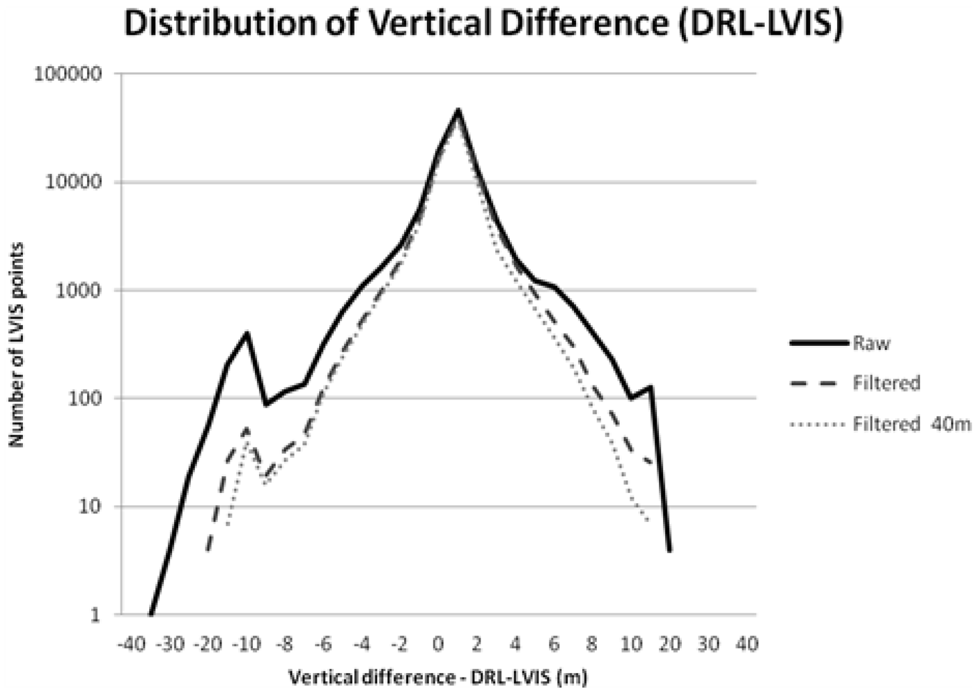
A total of 98,040 individual LFL last-pulse Zg points were compared with the DRL DEM (Table 3). A total of 337 (0.34%) LFL shots were outside the range of the DRL or exceeded the maximum parameters for DEM triangulation size. These points were not considered in the analysis. Comparison showed that the remaining 97,703 LFL shots were on average 28.7 cm lower (bias) than the DRL DEM, with a root mean square error (RMSE) of 2.33 m (‘Raw’ iteration in Table 1). This analysis provides encouraging results, showing that 95% (2 × RMSE) of the points are lying within 4.66 m of the actual ground surface observed by DRL, in all terrain types and canopy conditions (Figure 6). The comparison also highlights some of the main outliers of greater than 10 m that should clearly be removed from the DSM to create the DEM. While there was a small bias between the LFL and DRL ground elevation, the difference could reach to 35.68 m overestimation, or 16.38 m underestimation by LVIS. There were a number of instances where LFL signal saturates high in the canopy (>25 m), which are shown in the peak of the vertical difference, however on average the LFL pulses were lower than the DRL surface, presumably due to slope and topography. The bias may also be systematic within the LVIS sensor itself but cannot be readily determined unless we perform additional GPS elevation assessment over flat, paved, non-vegetated targets to test the vertical accuracy in comparison to DRL. Such targets do not exist in the overlapping regions of LFL and DRL data over BCI.
3.2. Establishing Empirical Relationships between Terrain Slope and LVIS LFL Zg Vertical Accuracy
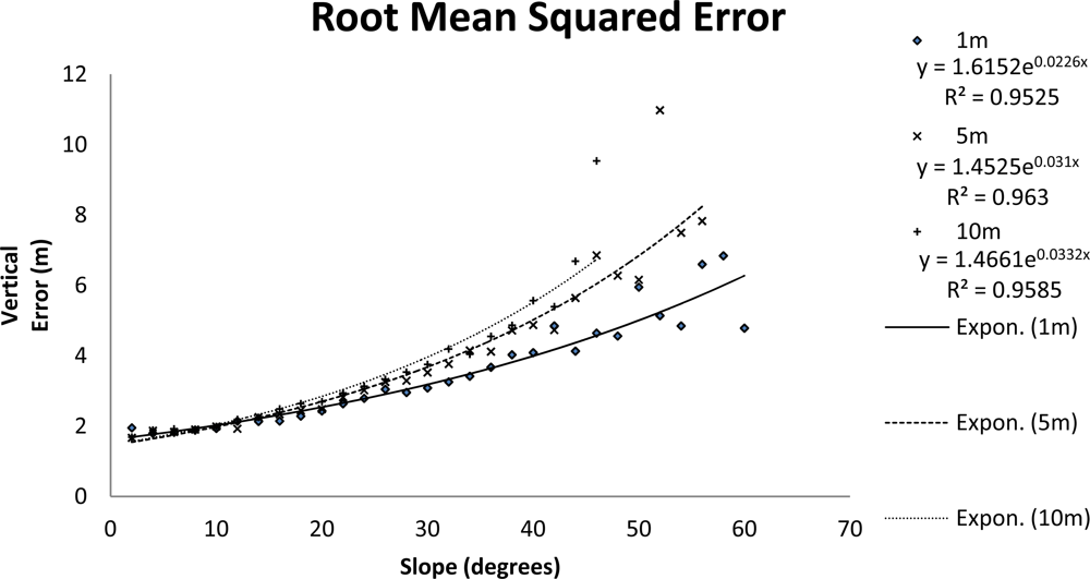
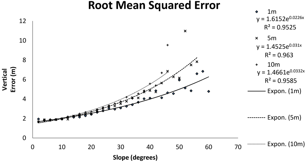
The terrain slope analysis showed an exponential degradation of LFL ground detection accuracy as terrain slope increased. The analysis was performed using three independent slope maps made at 1, 5 and 10 m resolutions. The coarser the resolution of the underlying DEM and subsequent slope map, the less extreme the LFL vertical errors appeared to be. When a fine spatial resolution was used to determine the slope at the center of the LFL footprint, the LFL vertical errors were larger. In general, the coarser resolution DEM will produce lower average slope across the landscape by overlooking small undulations in the ground surface or micro topography. The relationship between the errors in LFL DEM with respect to terrain slopes is shown in Figure 7. The corrections for slope are far less significant in terms of vertical differences compared to the large outliers removed in the filtering algorithms. However, slope corrections are more widespread and are applied to all LFL pulses.
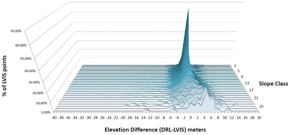
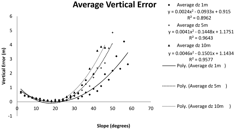
The analysis suggests that the average vertical error between LFL Zg elevations and the DRL DEM is a slightly parabolic function of the terrain slope (Figure 8), with flatter areas yielding more error than surfaces which are gently sloped (∼20 degrees) and with errors increasing progressively and becoming more variable at higher slopes (Figure 9). This implies that in flat areas, LFL is slightly underestimating ground elevation, although they have lowest level of variance. Based on our examination of the data, we found a systematic bias in vertical error between the two sensors. However the exact cause has yet to be determined. This is manifested by the parabolic bend between these slope ranges. It is possible that if slightly taller trees are present on moderate slopes of 10–25 degrees, the overall accuracy of LFL Zg points will be skewed more in the positive direction due to large trees resulting in additional ‘high’ LFL points compared to flat terrain. Previous research has suggested that multilayered forest stands on slopes and ridges, are often taller compared to valley stands, some of which are mono-layered [38]. A systematic bias between LFL points at the edge of the swath compared to points in the middle of the swath could result due to the scanning angle of LVIS. The use of a LFL calibration flight to collect data over large flat open surfaces could potentially provide extra assurance that there is no systematic bias in the LFL vertical accuracy.
3.3. Filtering of LVIS Zg Elevation Data
By filtering the LFL points using only the automated process (Figure 10), we found 11,234 points (11.46%) misrepresenting the ground surface and identified for further adjustment (‘Automatic Filtering’ iteration in Table 1). The most effective semi-automated process includes pre-filtering using the automatic filters, vertical adjustment based on terrain slope and a final post-processing filter. It results in 11,643 (11.88% of total) points removed from the DEM, resulting in a standard deviation of 1.605 m (‘Filtered->Slope Corrected->Filtered’ iteration in Table 1). To further improve the accuracy of the sub-canopy DEM, an additional visual inspection and manual editing to remove non-ground points which were not removed by the filters was performed. The filters have more success removing high-points rather than low points. The maximum elevation is a single LFL Zg point above the ground surface is 35.7 m, which decreases to 21.06 m after filtering. Conversely, the maximum elevation of a LFL Zg point below the ground surface was 16.4 m, which only decreased to 13.7 m after filtering. The preferential removal of these high points skewed the average difference towards an increasing vertical bias between LFL and DRL. Before filtering, LFL was an average of 28.2 cm lower than the DRL DEM. After using the semi-automated filtering process, the average vertical difference decreased to 13 cm lower than DRL DEM. The RMS decreased from 2.3 m to 1.6 m after the semi-automatic filtering. It indicates the new LFL processing methodology both increases average LFL accuracy and reduces variance.
The filtering algorithms eliminated the majority of points which were vastly different than the surrounding LVIS LFL points (Table 1). The combination of a low point and high point filtering algorithm managed to decrease the average error in the ground height measurements and significantly improved the sub-canopy DEM. To address the effectiveness of the LFL point filters at the edges of the island, we added two LFL filtering iterations. These only included points within the interior of BCI, 20 and 40 m from the shoreline (‘Filtered Interior −20 m/−40 m’ iterations in Table 1). A noticeable increase in LFL ground detection error occurs on the coastlines of the island, or at flight line edges or cloud gaps where LFL points have fewer neighboring points. The results indicate that the filtered interior points provide a more accurate representation of the actual ground surface than including LFL shots on the shorelines. All the tested measures of variance (average magnitude, RMS and standard deviation) decrease as fewer shoreline LFL points are analyzed. Average vertical difference between LFL and DRL also decreases when edge effects were excluded. The results indicate that the most extreme points lower than the ground surfaces were almost all on the coastlines, while high-points were generally inland. After filtering, only 9 of 32 LFL low points with errors greater than 10 m vertically were on the interior of the island and the majority of the extreme low point errors from 5 to 10 m vertical difference were on the coastlines. High points on the other hand were more concentrated in the interior of the island and were much easier to identify. However both high and low points with vertical errors of less than 6.5 m were difficult to identify visually. A particularly large number of double-bounce LFL measurements at the coastlines may systematically bias the data, particularly in an environment like BCI which has a very large coastline. Such an effect might be particularly important in coastal forests such as mangroves. The systematic average error bias may be explained by these edge effects, and further research is necessary to determine the importance of these errors.
If filtering algorithms are too aggressive in removing outlier points, ground points can be filtered out, resulting in an artificial flattening of topography. The filtering methodology in this study is relatively simple, only using two distinct steps to remove high and low points. The methodology can potentially be refined and adjusted to account for terrain slope, using more aggressive point filters in flat terrain and more conservative filters in steep terrain. As the LFL point filtering algorithms are refined, the time and attention required for a manual editing process will likely be reduced. Additional refinements of the presented methods are highly encouraged and we plan to test our methods in different study sites and more highly variable terrain. Although the highest topographic variation on BCI is in the stream gullies and at the edge of the plateau, there are no large topographic breaks or large sub-canopy features. A similar study in a tall, dense forest on steep terrain would expand our understanding of the empirical relationships between slope and LFL ground detection accuracy.
The results of this study are encouraging for future LFL studies and implementation of filtering processes should be considered in any case where ground penetration of the LFL pulses do not create a smooth initial DSM. By visualizing the last detected mode points in a DSM, large errors will become apparent. If such errors are visible, the LFL points should be filtered and the resulting waveforms should be corrected. If these errors go uncorrected, the corresponding canopy height measurements will be biased. In less dense forests with open canopies and sparse tree spacing, a visual inspection of the LFL Zg DSM may reveal fewer errors and filtering may be less important.
This methodology does not address canopy height directly, but rather ground elevation and the subsequent adjustment of the waveform data resulting from incorrect Zg elevation accuracy. Improvements in the sub-canopy DEM may be applied to the associated LFL waveform metrics to improve the quantification of the vertical canopy structure. Since all waveform metrics are referenced to the Zg elevation, the waveforms whose Zg value is determined to be significantly different from the ground must be recalculated. Although the canopy top (rh100) value can be accurately adjusted, there is no attempt to recalculate intermediate waveform metrics (rh25, rh50, rh75). The waveform relative height (rh) metrics can potentially be recalculated by adding the vertical elevation difference between DRL-LFL to the waveform profile in waveforms whose Zg values are below the ground surface. However the waveforms whose Zg values are above the ground will be difficult to recalculate due to the lack of waveform signal from the Zg elevation to the ground [7].
The empirical relationships between terrain slope and LFL vertical accuracy provide equations to predict expected errors and a method to adjust LFL ground heights based on terrain slope. Even in the absence of a DRL survey, a filtered LFL DEM can provide slope estimations which improve the average vertical accuracy compared with a raw LFL Zg DSM. Particular attention should be given to LFL laser pulses which do not reach the ground surface and emerge as significant ‘high point’ outliers after filtering. It is possible that these ‘high points’ deserve additional analysis, as they represent the tallest and densest parts of the forest canopy where light is significantly occluded from the ground surface. Implications of inaccurate LFL last-pulse in tall forests with high canopy closure can be significant to biomass estimates. Lastly, the LFL structural information and filtered DEMs should serve as a baseline surface for forest monitoring and change detection, which would be highly complementary to multiple types of remote sensing including multi-spectral, hyperspectral, multi-angle and repeat-pass IfSAR. The fusion of filtered LFL DEMs and other types of remote sensing will require further research.
This study had the benefit of having a high-density DRL survey which gave a high-resolution, high accuracy DEM for cross validation. The use of DRL to provide highly accurate measurements of forest structure and topography make it an invaluable calibration tool. However the lack of spatial coverage and the cost associated with DRL collection make it impractical for regional/global forest monitoring. When these data are available, highly accurate filtering algorithms can be written which use the DRL DEM to calibrate DRL. However, these filtering algorithms are designed to be used in the absence of such a high resolution DRL survey and are expected to stand-alone in order to be considered a viable solution for future wide-area LFL mapping missions. LFL is a more practical method for collecting wide areas from high-altitudes and has proven to be highly correlated with DRL metrics [17,29]. Studies using DRL and LFL in Costa Rica have shown that there is immense potential of lidar technology for tropical rain forest research and monitoring efforts [7,23,28–30,39].
Remote sensing based height estimates of the tropical forest canopy have a variety of potential applications such as determining canopy surface roughness [40], modeling light penetration [41], mapping wildlife habitat [42] and studying forest dynamics, such as gap formation, distribution and turn-over [43]. Lidar remote sensing has been used to characterize vertical changes in structure due to invasive species [18] and has been fused with hyperspectral imagery to further characterize tropical rain forest dynamics [21,39,44]. Lidar remote sensing should be considered for habitat characterization and suitability studies, particularly to avifauna. Ecological theory suggests that the vertical distribution of the forest canopy is the most important attribute for many canopy dwelling species [45]. Vegetation height is allometrically related to forest structure parameters such as estimated aboveground biomass [46] and size-frequency spatial distribution curves [47]. More recently, Asner et al. have proposed a universal airborne lidar approach for tropical forest carbon mapping using DRL which will potentially be applied to international efforts such as UN-REDD. The methods utilize DRL to characterize biomass to a high degree of certainty in four different tropical forests around the world. However, this approach may not be applicable to coarser resolution airborne and spaceborne LFL [4]. This study highlights the need to further develop LFL processing and filtering techniques in order to bridge the spatial gap between low-altitude DRL and regional airborne and spaceborne LFL mapping efforts to support UN-REDD goals.
4. Conclusions
The primary aim of this study was to develop a methodology to quantitatively correct sub-canopy elevation derived from large-footprint lidar data in dense tropical forests using small footprint discrete-return lidar measurements. The correction reduced the average digital elevation model error and variance significantly, particularly over sloped terrain. Majority (about 82%) of large-footprint lidar last-returns were within 2 meters of the discrete-return lidar detected ground surface, indicating the high accuracy of large-footprint lidar measurements in dense tropical forests. However, there were outliers and large errors particularly in areas of sloped terrain (about 18% of areas) with differences ranging from 16 to −35 m, with significantly positive bias (28 cm), suggesting relatively lower elevation than small footprint detected surface. By utilizing the filtering methods developed in this study, we improved most of the major outliers in large footprint elevation data and significantly reduced the digital elevation errors over Barro Colorado Island, Panama.
There is a strong correlation between terrain slope and large-footprint lidar ground detection accuracy. We developed an exponential model to approximate the elevation accuracy of large-footprint lidar last-return as a function of within footprint slope variation. The model can be used to predict average large-footprint lidar elevation biases and expected errors. Over the study area, the average vertical error in the large-footprint lidar elevation model was a parabolic function of terrain slope, suggesting a systematic bias between the lidar sensors. The shape and magnitude of the errors depend on the density of vegetation, underlying terrain slope, and potential double bounce interaction between vegetation and the sloped terrain. Forest edges next to bare surfaces such as the coastline at BCI may also create an ideal double-bounce environment for large-footprint lidar, causing a bias in detected elevation with respect to DRL digital elevation model. This testing should enable us to better quantify the nature of the parabolic average error function as it relates to terrain slope and edge effects.
From a lidar remote sensing perspective, Barro Colorado Island is a densely vegetated environment with well-studied old-growth Neotropical rainforest which provides some of the most difficult vegetation conditions large-footprint lidar is likely to encounter. Thus, the study’s results are encouraging and validate the ability of large-footprint lidar to accurately determine sub-canopy topography, and forest structure even under dense vegetation and topographic variation. The immediate implications of this study can impact how large-footprint lidar data is processed in the future. Implementation of filtering and slope correction methods will improve the data quality from the Laser Vegetation Imaging Sensor or similar large-footprint lidar sensors, designed for future NASA satellite sensors such as ICESAT-II or any future reincarnations Vegetation Canopy Lidar (VCL) or Deformation, Ecosystem Structure, and Dynamics of Ice (DESDynl). Steep topography and dense vegetation could be targeted as small calibration sites to be flown with discrete-return lidar and then used to refine filtering algorithms and vertical slope adjustments.
Improvements in the large-footprint lidar derived sub-canopy digital elevation model in heavily vegetated environments are a prerequisite to accurate large-scale tropical forest monitoring efforts. The authors are not aware of previous attempts to apply discrete-return lidar point cloud filtering techniques and sub-canopy ground detection methods to a large-footprint lidar forest survey. This study is a proof-of-concept at this stage and further research is necessary to further quantify the impacts of variable topography, high canopy closure, data gaps and vegetated shorelines. In areas of high relief, prior knowledge of terrain and ground control data will help future large-footprint lidar sub-canopy detection efforts. Future efforts to accurately measure forest structure using large-footprint lidar in dense forest conditions should focus on algorithm development, waveform analysis, extreme terrain and investigation into the heterogeneous spatial distribution of the double-bounce phenomenon occurring at the edge of the forest. The results of this study present a repeatable method to improve large-footprint lidar forest structure measurements by creating a more accurate sub-canopy digital elevation model.
Acknowledgments
The authors thank Jim Dalling who generously provided the BCI DRL dataset to our research team. J. B. Blair generously offered help and guidance for LVIS data processing and Richard Condit and Stephen Hubbell provided information about the field survey data in the 50-ha plot. Evan Lyons and Vena Chu assisted the project with technical programming expertise. This research would not be possible without Todd Stennett, Bryant Bertrand, Arthur Edwards, Sean Bowers, Jerome Gregory and Donovan Tunay of Airborne 1, for providing data processing tools, data storage and use of company facilities and resources. Chuck Anderson, Mark Hanus, Olavi Kelle and Alastair Jenkins of Geodigital International Corporation were very generous in providing material support, as well as guidance and advice. Gregory Okin and Marc Simard for scientific guidance and research design. We owe Nicole Corpuz an extended credit for her work, performing the manual LVIS DSM editing and Chelsea Robinson for reviewing the manuscript and providing notes.
Data set acknowledgement: Data sets were provided by the Laser Vegetation Imaging Sensor (LVIS) team in the Laser Remote Sensing Branch at NASA Goddard Space Flight Center with support from the University of Maryland, College Park. Authors: J. Bryan Blair, NASA Goddard Space Flight Center, David Lloyd Rabine, SSAI at GSFC, Michelle Hofton, University of Maryland College Park. http://lvis.gsfc.nasa.gov.
Funding for the collection and processing of the 1998 Central America data were provided by the Vegetation Canopy Lidar (VCL) Science team (NASA grant number NAS597160) and NASA’s Interdisciplinary Science Program (IDS) (NASA grant number NNG04GO05G). Publisher: Code 694 NASA Goddard Space Flight Center. ESRI world map data (Figure 1).
References
- Ranson, K.J.; Sun, G. Mapping biomass of a northern forest using multifrequency SAR data. IEEE Trans. Geosci. Remote Sens 1994, 32, 388–396. [Google Scholar]
- Imhoff, M.L. Radar backscatter and biomass saturation: Ramifications for global biomass inventory. IEEE Trans. Geosci. Remote Sens 1995, 33, 511–518. [Google Scholar]
- Gibbs, H.K.; Brown, S.; Niles, J.O.; Foley, J.A. Monitoring and estimating tropical forest carbon stocks: Making redd a reality. Environ. Res. Lett 2007, 2, 045023. [Google Scholar]
- Asner, G.; Mascaro, J.; Muller-Landau, H.; Vieilledent, G.; Vaudry, R.; Rasamoelina, M.; Hall, J.; van Breugel, M. A universal airborne lidar approach for tropical forest carbon mapping. Oecologia 2012, 168, 1147–1160. [Google Scholar]
- Lefsky, M.A.; Cohen, W.B.; Parker, G.G.; Harding, D.J. Lidar remote sensing for ecosystem studies. BioScience 2002, 52, 19–30. [Google Scholar]
- Turner, W.; Spector, S.; Gardiner, N.; Fladeland, M.; Sterling, E.; Steininger, M. Remote sensing for biodiversity science and conservation. Trends Ecol. Evol 2003, 18, 306–314. [Google Scholar]
- Blair, J.B.; Rabine, D.L.; Hofton, M.A. The laser vegetation imaging sensor: A medium-altitude, digitisation-only, airborne laser altimeter for mapping vegetation and topography. ISPRS J. Photogramm 1999, 54, 115–122. [Google Scholar]
- Sheng, Y. Quantifying the size of a lidar footprint: A set of generalized equations. IEEE Geosci. Remote Sens. Lett 2008, 5, 419–422. [Google Scholar]
- Saatchi, S.S.; Harris, N.L.; Brown, S.; Lefsky, M.; Mitchard, E.T.A.; Salas, W.; Zutta, B.R.; Buermann, W.; Lewis, S.L.; Hagen, S.; et al. Benchmark map of forest carbon stocks in tropical regions across three continents. Proc. Natl. Acad. Sci 2011, 108, 9899–9904. [Google Scholar]
- Lefsky, M.A. A global forest canopy height map from the moderate resolution imaging spectroradiometer and the geoscience laser altimeter system. Geophys. Res. Lett 2010, 37, L15401. [Google Scholar]
- Simard, M.; Zhang, K.; Rivera-Monroy, V.H.; Ross, M.S.; Ruiz, P.L.; Castaneda-Moya, E.; Twilley, R.R.; Rodriguez, E. Mapping height and biomass of mangrove forests in everglades national park with srtm elevation data. Photogramm. Eng. Remote Sensing 2006, 72, 299–311. [Google Scholar]
- Harding, D.J.; Carabajal, C.C. IceSat waveform measurements of within-footprint topographic relief and vegetation vertical structure. Geophys. Res. Lett 2005, 32, L21S10. [Google Scholar]
- Lefsky, M.A.; Keller, M.; Pang, Y.; De Camargo, P.B.; Hunter, M.O. Revised method for forest canopy height estimation from geoscience laser altimeter system waveforms. J. Appl. Remote Sens 2007, 1, 013537–013518. [Google Scholar]
- Carabajal, C.C.; Harding, D.J.; Suchdeo, V.P. IceSat Lidar and Global Digital Elevation Models: Applications to DesDyni. Proceedings of 2010 IEEE International Geoscience and Remote Sensing Symposium (IGARSS), Honolulu, HI, USA, 25–30 July 2010; pp. 1907–1910.
- Chen, Q. Assessment of terrain elevation derived from satellite laser altimetry over mountainous forest areas using airborne lidar data. ISPRS J. Photogramm 2010, 65, 111–122. [Google Scholar]
- Dubayah, R.O.; Drake, J.B. Lidar remote sensing for forestry. J. For 2000, 98, 44–46. [Google Scholar]
- Clark, M.L.; Clark, D.B.; Roberts, D.A. Small-footprint lidar estimation of sub-canopy elevation and tree height in a tropical rain forest landscape. Remote Sens. Environ 2004, 91, 68–89. [Google Scholar]
- Asner, G.P.; Hughes, R.F.; Vitousek, P.M.; Knapp, D.E.; Kennedy-Bowdoin, T.; Boardman, J.; Martin, R.E.; Eastwood, M.; Green, R.O. Invasive plants transform the three-dimensional structure of rain forests. Proc. Natl. Acad. Sci 2008, 105, 4519–4523. [Google Scholar]
- Kellner, J.R.; Clark, D.B.; Hubbell, S.P. Pervasive canopy dynamics produce short-term stability in a tropical rain forest landscape. Ecol. Lett 2009, 12, 155–164. [Google Scholar]
- King, D.A. Allometry and life history of tropical trees. J. Trop. Ecol 1996, 12, 25–44. [Google Scholar]
- Drake, J.B.; Knox, R.G.; Dubayah, R.O.; Clark, D.B.; Condit, R.; Blair, J.B.; Hofton, M. Above-ground biomass estimation in closed canopy neotropical forests using lidar remote sensing: Factors affecting the generality of relationships. Global Ecol. Biogeogr 2003, 12, 147–159. [Google Scholar]
- Dubayah, R.; Prince, S.; Jaja, J.; Blair, J.B.; Bufton, J.L.; Knox, R.; Luthcke, S.B.; Clark, D.B.; Weishampel, J.F. The Vegetation Canopy Lidar Mission. Proceedings of Land Satellite Information in the Next Decade II: Sources and Applications, Washington, DC, USA, 2–5 December 1997; pp. 2–5.
- Hofton, M.A.; Rocchio, L.E.; Blair, J.B.; Dubayah, R. Validation of vegetation canopy lidar sub-canopy topography measurements for a dense tropical forest. J. Geodynam 2002, 34, 491–502. [Google Scholar]
- Zhang, K.; Chen, S.-C.; Whitman, D.; Shyu, M.-L.; Yan, J.; Zhang, C. A progressive morphological filter for removing nonground measurements from airborne lidar data. IEEE Trans. Geosci. Remote Sens 2003, 41, 872–882. [Google Scholar]
- Zhang, K.; Whitman, D. Comparison of three algorithms for filtering airborne lidar data. Photogramm. Eng. Remote Sensing 2005, 71, 313–324. [Google Scholar]
- Sithole, G.; Vosselman, G. Experimental comparison of filter algorithms for bare-earth extraction from airborne laser scanning point clouds. ISPRS J. Photogramm 2004, 59, 85–101. [Google Scholar]
- Flood, M. Lidar activities and research priorities in the commercial sector. Int. Arch. Photogramm. Remote Sens. Spatial Inf. Sci 2001, 34, 3–8. [Google Scholar]
- Drake, J.B.; Dubayah, R.O.; Knox, R.G.; Clark, D.B.; Blair, J.B. Sensitivity of large-footprint lidar to canopy structure and biomass in a neotropical rainforest. Remote Sens. Environ 2002, 81, 378–392. [Google Scholar]
- Drake, J.B.; Dubayah, R.O.; Clark, D.B.; Knox, R.G.; Blair, J.B.; Hofton, M.A.; Chazdon, R.L.; Weishampel, J.F.; Prince, S. Estimation of tropical forest structural characteristics using large-footprint lidar. Remote Sens. Environ 2002, 79, 305–319. [Google Scholar]
- Weishampel, J.F.; Blair, J.B.; Knox, R.G.; Dubayah, R.; Clark, D.B. Volumetric lidar return patterns from an old-growth tropical rainforest canopy. Int. J. Remote Sens 2000, 21, 409–415. [Google Scholar]
- Lim, K.; Treitz, P.; Wulder, M.; St-Onge, B.; Flood, M. Lidar remote sensing of forest structure. Progr. Phys. Geogr 2003, 27, 88–106. [Google Scholar]
- Clark, D.B.; Clark, D.A. Landscape-scale variation in forest structure and biomass in a tropical rain forest. For. Ecol. Manage 2000, 137, 185–198. [Google Scholar]
- Croat, T.B. Flora of Barro Colorado Island; Stanford University Press: Stanford, CA, USA, 1978. [Google Scholar]
- Condit, R. Research in large, long-term tropical forest plots. Trends Ecol. Evol 1995, 10, 18–22. [Google Scholar]
- Condit, R. Tropical Forest Census Plots: Methods and Results from Barro Colorado Island, Panama and a Comparison with Other Plots; Springer: Berlin, Germany, 1998. [Google Scholar]
- Ahmed, R.; Siqueira, P.; Bergen, K.; Chapman, B.; Hensley, S. A Biomass Estimate over the Harvard Forest Using Field Measurements with Radar and Lidar Data. Proceedings of 2010 IEEE International Geoscience and Remote Sensing Symposium (IGARSS), Honolulu, HI, USA, 25–30 July 2010; pp. 4768–4771.
- Hubbell, S.P.; Foster, R.B.; O’Brien, S.T.; Harms, K.E.; Condit, R.; Wechsler, B.; Wright, S.J.; de Lao, S.L. Light-gap disturbances, recruitment limitation, and tree diversity in a neotropical forest. Science 1999, 283, 554–557. [Google Scholar]
- Gale, N. The relationship between canopy gaps and topography in a western ecuadorian rain forest1. Biotropica 2000, 32, 653–661. [Google Scholar]
- Clark, M.L.; Roberts, D.A.; Ewel, J.J.; Clark, D.B. Estimation of tropical rain forest aboveground biomass with small-footprint lidar and hyperspectral sensors. Remote Sens. Environ 2011, 115, 2931–2942. [Google Scholar]
- Raupach, M.R. Simplified expressions for vegetation roughness length and zero-plane displacement as functions of canopy height and area index. Bound.-Lay. Meteorol 1994, 71, 211–216. [Google Scholar]
- Montgomery, R.A.; Chazdon, R.L. Forest structure, canopy architecture, and light transmittance in tropical wet forests. Ecology 2001, 82, 2707–2718. [Google Scholar]
- Hinsley, S.A.; Hill, R.A.; Gaveau, D.L.A.; Bellamy, P.E. Quantifying woodland structure and habitat quality for birds using airborne laser scanning. Functional Ecology 2002, 16, 851–857. [Google Scholar]
- Birnbaum, P. Canopy surface topography in a French guiana forest and the folded forest theory. Plant Ecology 2001, 153, 293–300. [Google Scholar]
- Clark, M.L.; Roberts, D.A.; Clark, D.B. Hyperspectral discrimination of tropical rain forest tree species at leaf to crown scales. Remote Sens. Environ 2005, 96, 375–398. [Google Scholar]
- Hyde, P.; Dubayah, R.; Peterson, B.; Blair, J.B.; Hofton, M.; Hunsaker, C.; Knox, R.; Walker, W. Mapping forest structure for wildlife habitat analysis using waveform lidar: Validation of montane ecosystems. Remote Sens. Environ 2005, 96, 427–437. [Google Scholar]
- Clark, D.B.; Read, J.M.; Clark, M.L.; Cruz, A.M.; Dotti, M.F.; Clark, D.A. Application of 1-m and 4-m resolution satellite data to studies of tree demography, stand structure and land-use classification in tropical rain forest landscapes. Ecol. Appl 2004, 14, 61–74. [Google Scholar]
- West, G.B.; Enquist, B.J.; Brown, J.H. A general quantitative theory of forest structure and dynamics. Proc. Natl. Acad. Sci 2009, 106, 7040–7045. [Google Scholar]
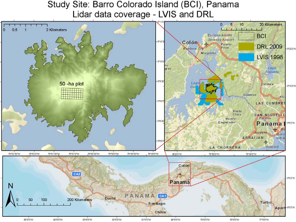
Figure 1.
Study Site: Barro Colorado Island (BCI) and the 50-ha Forest Dynamics Plot (top-left) and the discrete-return lidar (DRL) derived hillshade model to show relief, regional lidar data coverage (top-right), Republic of Panama (bottom).
Figure 1.
Study Site: Barro Colorado Island (BCI) and the 50-ha Forest Dynamics Plot (top-left) and the discrete-return lidar (DRL) derived hillshade model to show relief, regional lidar data coverage (top-right), Republic of Panama (bottom).

Figure 2.
The four-step methodology for improving large-footprint lidar (LFL) sub-canopy digital elevation model (DEM) and associated waveform canopy metrics. Data sets are in the upper-left (light grey) and data products are in the bottom-right (dark grey).
Figure 2.
The four-step methodology for improving large-footprint lidar (LFL) sub-canopy digital elevation model (DEM) and associated waveform canopy metrics. Data sets are in the upper-left (light grey) and data products are in the bottom-right (dark grey).

Figure 3.
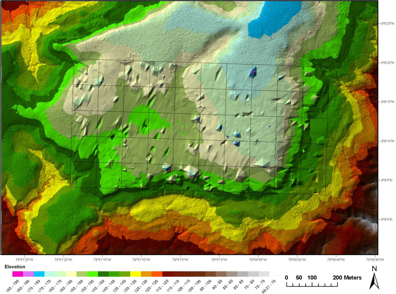
Two Triangulated Irregular Network (TIN) digital surface models colored by elevation. Inside the 50-ha plot (black grid) the coarse scale unfiltered LFL digital-surface model (DSM) and the fine scale control DRL DEM surface outside the 50-ha plot.
Figure 3.
Two Triangulated Irregular Network (TIN) digital surface models colored by elevation. Inside the 50-ha plot (black grid) the coarse scale unfiltered LFL digital-surface model (DSM) and the fine scale control DRL DEM surface outside the 50-ha plot.

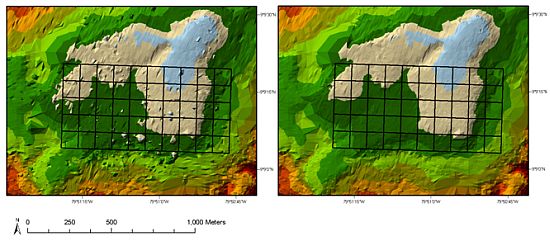
Figure 4.
Map of DRL–derived slope on BCI at three spatial resolutions, 1 m (left), 5 m (center), 10 m (right). LFL laser pulse center points are displayed on slope map to display the variation in terrain at different spatial resolutions.
Figure 4.
Map of DRL–derived slope on BCI at three spatial resolutions, 1 m (left), 5 m (center), 10 m (right). LFL laser pulse center points are displayed on slope map to display the variation in terrain at different spatial resolutions.

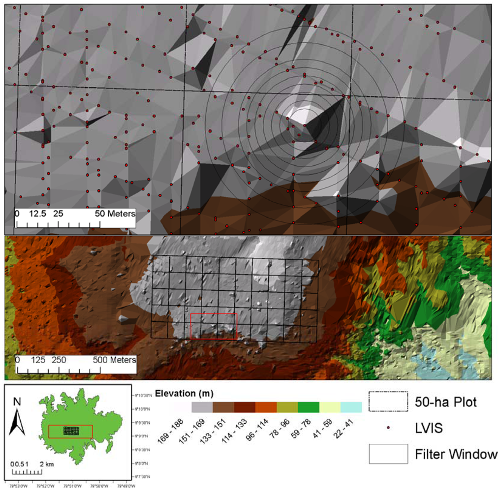
Figure 5.
The iterative expanding windows (solid concentric circles) used by the filtering process is shown around a visually significant outlier LFL center point within the 50-ha plot (top). Concentric expanding windows occur at 10, 15, 20, 25, 30, 35, 40, 50 and 60 m. The filtering process is applied to all LFL Zg points across the island (middle/bottom).

Figure 6.
Distribution of vertical errors between LFL Zg values and the DRL DEM. Filtered 20 and 40 m indicate only LFL Zg values that have been filtered and sampled from the interior of the island, 20 and 40 m from the shoreline respectively. Negative numbers indicate the LFL Zg value is above the ground surface. The y-axis is logarithmic to accentuate the edges of the histogram.

Figure 7.
Average vertical difference (x-axis) between LFL and DRL DEM (m), as a function of terrain slope by relative percentage of LFL points in each slope class. Negative vertical difference values indicate LFL points are higher than DRL DEM, i.e., DRL – LFL = vertical difference. Percentage of LFL points in each slope class (y-axis.) Flat terrain is represented at the back of the chart and increasing in steepness towards the front (z-axis). Each slope class is a 2 degree interval. Examined at 1 m pixel resolution.

Figure 8.
Average Vertical Error between LFL and DRL derived DEMs, as a function of terrain slope. Difference in vertical elevation (dz) between DRL DEM and LFL Zg., examined at three pixel sizes (1 m, 5 m, 10 m).
Figure 8.
Average Vertical Error between LFL and DRL derived DEMs, as a function of terrain slope. Difference in vertical elevation (dz) between DRL DEM and LFL Zg., examined at three pixel sizes (1 m, 5 m, 10 m).
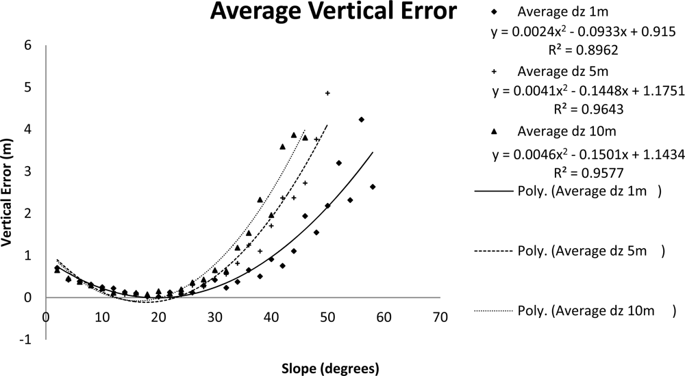
Figure 9.
Root Mean Squared Error between LFL and DRL derived DEMs, as a function of terrain slope, examined at three pixel sizes (1 m, 5 m, 10 m).
Figure 9.
Root Mean Squared Error between LFL and DRL derived DEMs, as a function of terrain slope, examined at three pixel sizes (1 m, 5 m, 10 m).

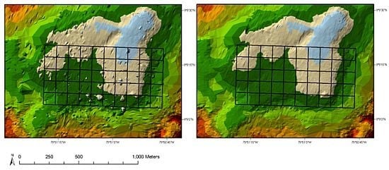
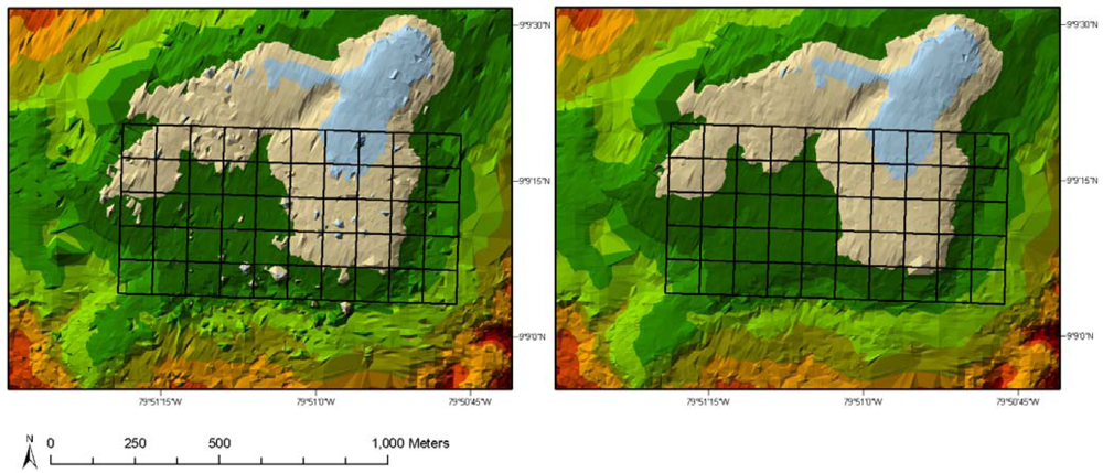
Figure 10.
Results of the fully-automated point filtering algorithms without manual editing (Iteration ‘Automatic Filtering’ in Table 1) in the area of the 50-ha forest dynamics plot on BCI. Raw unfiltered DSM (left), Filtered DEM (right).
Figure 10.
Results of the fully-automated point filtering algorithms without manual editing (Iteration ‘Automatic Filtering’ in Table 1) in the area of the 50-ha forest dynamics plot on BCI. Raw unfiltered DSM (left), Filtered DEM (right).


Table 1.
Technical description of the Low Point filter used to identify LFL Zg points below the ground surface.
| Low Point Filter | ||||||||
|---|---|---|---|---|---|---|---|---|
| Filtering Iteration | Routine | From | To | Search for | Vertical Threshold (m) | Search Radius (m) | Limit STDEV | Z-Tolerance |
| 1 | ClassifyLow | LVIS_GRND | LVIS_ZG | single point | 2 | 15 | NA | NA |
| 2 | ClassifyLow | LVIS_GRND | LVIS_ZG | single point | 3 | 20 | NA | NA |
| 3 | ClassifyLow | LVIS_GRND | LVIS_ZG | single point | 3 | 25 | NA | NA |
| 4 | ClassifyLow | LVIS_GRND | LVIS_ZG | single point | 3 | 30 | NA | NA |
| 5 | ClassifyLow | LVIS_GRND | LVIS_ZG | single point | 3.5 | 35 | NA | NA |
| 6 | ClassifyLow | LVIS_GRND | LVIS_ZG | group of points | 2 | 15 | NA | NA |
| 7 | ClassifyLow | LVIS_GRND | LVIS_ZG | group of points | 3 | 20 | NA | NA |
| 8 | ClassifyBelow | LVIS_GRND | LVIS_ZG | single point | 3 | NA | 3 | 5 |
| 9 | ClassifyBelow | LVIS_GRND | LVIS_ZG | single point | 4 | NA | 4 | 4 |
Table 2.
Technical description of the High Point filter used to identify LFL Zg points above the ground surface.
| High Point Filter | ||||||||
|---|---|---|---|---|---|---|---|---|
| Filtering Iteration | Routine | From | To | Search for | Vertical Threshold (m) | Search Radius (m) | Points Required | Limit STDEV |
| 1 | ClassifyAir | LVIS_GRND | LVIS_ZG | single point | 2 | 10 | 3 | 1 |
| 2 | ClassifyAir | LVIS_GRND | LVIS_ZG | single point | 3 | 15 | 3 | 1.5 |
| 3 | ClassifyAir | LVIS_GRND | LVIS_ZG | single point | 3 | 20 | 3 | 1.5 |
| 4 | ClassifyAir | LVIS_GRND | LVIS_ZG | single point | 3 | 25 | 4 | 2 |
| 5 | ClassifyAir | LVIS_GRND | LVIS_ZG | single point | 3.5 | 30 | 5 | 2.5 |
| 6 | ClassifyAir | LVIS_GRND | LVIS_ZG | group of points | 2 | 40 | 7 | 2 |
| 7 | ClassifyAir | LVIS_GRND | LVIS_ZG | group of points | 3 | 50 | 15 | 2 |
| 8 | ClassifyAir | LVIS_GRND | LVIS_ZG | single point | 3 | 60 | 20 | 1.5 |
Table 3.
Multiple filtering iterations of Laser Vegetation Imaging Sensor (LVIS) LFL Zg points, including interior island and slope corrected points. All distance units are meters and the table is organized by increasing Root Mean Squared (RMS).
| Iteration | Total Points | Points Removed | % Removed | DRL-Zg | Minimum Change | Maximum | Ave Abs Change Value | RMS | STDEV |
|---|---|---|---|---|---|---|---|---|---|
| Filtered Interior −40 m | 76,056 | 21,984 | 22.42% | 0.33 | −18.26 | 13.57 | 0.986 | 1.505 | 1.469 |
| Filtered Interior −20 m | 81,315 | 16,725 | 17.06% | 0.36 | −18.26 | 13.57 | 1.006 | 1.533 | 1.490 |
| Filtering/Manual Editing | 86,363 | 11,677 | 11.91% | 0.44 | −18.98 | 14.90 | 1.049 | 1.580 | 1.517 |
| Filtered -> Slope | 86,397 | 11,643 | 11.88% | 0.13 | −21.33 | 14.97 | 0.997 | 1.610 | 1.605 |
| Corrected ->Filter | |||||||||
| Slope Corrected -> Filtered | 86,498 | 11,542 | 11.77% | 0.14 | −22.66 | 14.93 | 1.002 | 1.617 | 1.612 |
| Automatic Filtering | 86,806 | 11,234 | 11.46% | 0.42 | −21.06 | 14.90 | 1.067 | 1.645 | 1.589 |
| Manual Editing | 96,144 | 1,896 | 1.93% | 0.34 | −30.76 | 16.38 | 1.193 | 1.928 | 1.898 |
| Raw Interior (−20 m) | 92,074 | 5,966 | 6.09% | 0.22 | −35.68 | 16.38 | 1.289 | 2.309 | 2.298 |
| Raw Interior (−40 m) | 86,063 | 11,977 | 12.22% | 0.18 | −35.68 | 15.04 | 1.277 | 2.314 | 2.307 |
| Raw (Slope Corrected) | 97,788 | 252 | 0.26% | 0.00 | −35.85 | 16.33 | 1.273 | 2.318 | 2.318 |
| Raw | 98,040 | 0 | 0.00% | 0.28 | −35.68 | 16.38 | 1.325 | 2.329 | 2.312 |
Share and Cite
MDPI and ACS Style
Fricker, G.A.; Saatchi, S.S.; Meyer, V.; Gillespie, T.W.; Sheng, Y. Application of Semi-Automated Filter to Improve Waveform Lidar Sub-Canopy Elevation Model. Remote Sens. 2012, 4, 1494-1518. https://doi.org/10.3390/rs4061494
AMA Style
Fricker GA, Saatchi SS, Meyer V, Gillespie TW, Sheng Y. Application of Semi-Automated Filter to Improve Waveform Lidar Sub-Canopy Elevation Model. Remote Sensing. 2012; 4(6):1494-1518. https://doi.org/10.3390/rs4061494
Chicago/Turabian StyleFricker, Geoffrey A., Sassan S. Saatchi, Victoria Meyer, Thomas W. Gillespie, and Yongwei Sheng. 2012. "Application of Semi-Automated Filter to Improve Waveform Lidar Sub-Canopy Elevation Model" Remote Sensing 4, no. 6: 1494-1518. https://doi.org/10.3390/rs4061494