Preparing Landsat Image Time Series (LITS) for Monitoring Changes in Vegetation Phenology in Queensland, Australia


1
Biophysical Remote Sensing Group, Centre for Spatial Environmental Research, School of Geography, Planning and Environmental Management, The University of Queensland, Brisbane, QLD 4072, Australia
2
Indufor Asia Pacific Ltd, 55 Shortland St, PO Box 105039, Auckland , 1143, New Zealand
3
Remote Sensing Centre, Remote Sensing Unit, NSW Office of Environment and Heritage, P.O. Box 717, Dubbo, NSW 2830, Australia
*
Author to whom correspondence should be addressed.
Remote Sens. 2012, 4(6), 1856-1886; https://doi.org/10.3390/rs4061856
Submission received: 12 May 2012
/
Revised: 12 June 2012
/
Accepted: 15 June 2012
/
Published: 19 June 2012
Abstract
:Time series of images are required to extract and separate information on vegetation change due to phenological cycles, inter-annual climatic variability, and long-term trends. While images from the Landsat Thematic Mapper (TM) sensor have the spatial and spectral characteristics suited for mapping a range of vegetation structural and compositional properties, its 16-day revisit period combined with cloud cover problems and seasonally limited latitudinal range, limit the availability of images at intervals and durations suitable for time series analysis of vegetation in many parts of the world. Landsat Image Time Series (LITS) is defined here as a sequence of Landsat TM images with observations from every 16 days for a five-year period, commencing on July 2003, for a Eucalyptus woodland area in Queensland, Australia. Synthetic Landsat TM images were created using the Spatial and Temporal Adaptive Reflectance Fusion Model (STARFM) algorithm for all dates when images were either unavailable or too cloudy. This was done using cloud-free scenes and a MODIS Nadir BRDF Adjusted Reflectance (NBAR) product. The ability of the LITS to measure attributes of vegetation phenology was examined by: (1) assessing the accuracy of predicted image-derived Foliage Projective Cover (FPC) estimates using ground-measured values; and (2) comparing the LITS-generated normalized difference vegetation index (NDVI) and MODIS NDVI (MOD13Q1) time series. The predicted image-derived FPC products (value ranges from 0 to 100%) had an RMSE of 5.6. Comparison between vegetation phenology parameters estimated from LITS-generated NDVI and MODIS NDVI showed no significant difference in trend and less than 16 days (equal to the composite period of the MODIS data used) difference in key seasonal parameters, including start and end of season in most of the cases. In comparison to similar published work, this paper tested the STARFM algorithm in a new (broadleaf) forest environment and also demonstrated that the approach can be used to form a time series of Landsat TM images to study vegetation phenology over a number of years.
1. Introduction
Landsat, one of the longest running satellite programs has been acquiring images of the Earth’s surface since 1972. Although, there is a data continuity problem due to uncertainty over Landsat data continuity mission, failure of scan line corrector in Landsat 7 ETM+ and retirement of Landsat 5, the images collected by its Multispectral Scanner (MSS), Thematic Mapper (TM) and Enhanced Thematic Mapper Plus (ETM+) sensors have remained on the forefront of land-cover change monitoring and the development of various remote sensing applications [1]. The 30 m pixel size of the TM and ETM+ sensors makes them suitable to characterize the land-cover change resulting from natural and anthropogenic activities. Their number and placement of spectral bands is also an important advantage over other similar sensors. The TM and ETM+ sensors acquire the images in visible, near infrared and shortwave infrared portions of the electromagnetic spectrum, making them appropriate for studies of vegetation properties across a wide range of vegetation communities, in diverse environments [1–4].
Measuring, mapping and understanding changes in vegetation properties over specific spatial and temporal scales is critical for a range of ecosystem science and natural resource management applications. Remote sensing is considered a viable method for gathering information in a spatially and temporally continuous fashion. However, separating changes taking place due to phenological cycles, inter-annual climatic variability, human activities and long-term trends is challenging unless a data set of sufficient duration and short enough period between image acquisition dates exists. It is not possible with commonly used multi-temporal remote sensing applications, such as simple bi-temporal change detection and multi-date image analysis to extract this type of information [5–7]. Time series analysis techniques and data with highly frequent temporal observations sufficient for capturing seasonal variability (at least monthly) are required to produce such information [8,9]. Remote sensing sensors often trade-off between spatial and temporal resolution to acquire high spatial-resolution low repeat-frequency images, or low spatial-resolution high temporal-frequency images. Data from low spatial-resolution sensors like Advanced Very High Resolution Radiometer (AVHRR), Satellite Pour l’Observation de la Terre (SPOT)—VEGETATION, Moderate Resolution Imaging Spectroradiometer (MODIS) and Medium Resolution Imaging Spectrometer (MERIS) with spatial resolution ranging from 250 m to 1,000 m are acquired at high temporal-resolutions, making them a suitable source for time series analysis to monitor vegetation change [10–12]. Many processes of interest in terrestrial ecosystems operate at spatial scales below the spatial resolution of those sensors and are more suited to detection at Landsat TM and ETM+ scales [13].
A Landsat image time series (LITS) is defined here as a sequence of Landsat Thematic Mapper (TM) images produced for a particular area with the best possible geometric registration, radiometric consistency and sufficient temporal resolution. Preparation of such a data set has a series of challenges. Until recently, it was an expensive endeavor given the high purchase cost of data. The data cost is no longer an issue after the decision which has made all US Geological Survey (USGS), archived Landsat data freely available [14]. In a number of areas around the world frequent cloud cover and smoke haze, and seasonal limitations to the Landsat 5 acquisition cycle could significantly extend the time between two successive, usable images [15]. Similarly, the successive Landsat TM scenes may not be radiometrically and geometrically consistent. The individual Landsat TM scene may need a considerable pre-processing effort to achieve a high level of geometric and radiometric integrity required for a time series analysis [16].
Integration of higher temporal-resolution images from the MODIS sensors with available Landsat TM and ETM+ image by using image fusion techniques is one of the solutions for preparing LITS by filling the gaps in Landsat image sequence due to the cloud and other problems [17–19]. MODIS sensors on board the Terra and Aqua satellites acquire data in 36 bands with a near daily revisit cycle in most parts of the world [20]. Out of seven MODIS bands which are commonly used for terrestrial applications, six are spectrally similar to Landsat TM and ETM+ reflective bands [17,21]. Generally, the image fusion techniques integrate high temporal and/or spectral resolution images and high spatial-resolution images to increase the temporal and/or spectral resolution of high spatial-resolution images [22]. Although a number of image fusion techniques and algorithms are found in existing literature, very few are capable of producing scaled reflectance at higher spatial resolutions [17,18].
The Spatial and Temporal Adaptive Reflectance Fusion Model (STARFM) [17], Multi-temporal MODIS-Landsat data fusion method [18], Muti-Resolution Multi-Temporal technique [23] and Enhanced Spatial and Temporal Adaptive Reflectance Fusion Model (ESTARFM) [19] are capable of producing reflectance at Landsat TM and ETM+ spatial scales by integrating Landsat TM and MODIS reflectance. The STARFM algorithm predicts reflectance at Landsat TM and ETM+ spatial resolution using one or more pairs of Landsat and MODIS images acquired on the same date and MODIS reflectance from the date at which the Landsat TM reflectance is to be predicted [17]. The method has been tested in coniferous forests in British Columbia, Canada for predicting surface reflectance at Landsat TM spatial scale with reasonable accuracy when compared to actual Landsat TM reflectance [24]. The Multi-temporal MODIS-Landsat data fusion method estimates Landsat TM reflectance assuming that the temporal dynamics of MODIS reflectance can be approximated by a modulation term (ratio of reflectance between two dates), which remains representative of the temporal variation in reflectance at the Landsat TM pixel scale over the same period given the viewing and illumination geometry remains same [18]. The Multi-Resolution Multi-temporal technique estimates the reflectance based on percent contribution of Landsat pixels within the MODIS pixels [23]. Unlike STARFM, the methods have not been further tested and validated. ESTARFM is the enhanced version of the STARFM algorithm, which performs better in an environment with heterogeneous land-cover types at the MODIS pixel scale [19]. This method requires at least two pairs of fine and coarse spatial-resolution data acquired at the same date as input, whereas STARFM can work with a single pair. The minimum requirement of two pairs of images could be a limitation of ESTARFM. Finding two sets of high quality inputs is difficult as images of proximal dates representing different stages of phenological changes are desirable for better prediction results [19].
Gao et al. [17] originally tested the STARFM algorithm in a boreal forest environment using MODIS daily surface reflectance (MOD09GHK) as MODIS input reflectance. Hilker et al. [24] further tested the algorithm [17] to predict a small number of Landsat images within a period of five months using MODIS eight-day composite reflectance (MOD09A1) products in a coniferous-dominated environment. However, to date, the algorithm has not been used to generate a long, regularly-spaced time series of data, spanning several seasonal cycles, suitable for vegetation phenology studies, outside of coniferous-dominated environments [24].
The aim of this work was to construct a long (2003–2008) time series of Landsat TM images (LITS) for assessing vegetation phenology in Eucalyptus woodland and open forest environments in Australia. To achieve the aim, three specific tasks were addressed. The first task was to work out a pre-processing routine to make all available Landsat TM images geometrically and radiometrically consistent and suitable for input to the STARFM algorithm [17] to fill the gap in the time series. The second task was to use STARFM algorithm to predict synthetic images for all dates when Landsat TM images were not captured or unsuitable using an appropriate MODIS reflectance product and nearest-date Landsat TM imagery. The second task was also to examine the accuracy of the synthetic reflectance by direct comparison to observed image-reflectance, and by deriving foliage projective cover estimates from the imagery and comparing it to field-measured estimates of tree-foliage density. The final task was to assess the ability of LITS to monitor changes in vegetation phenology by comparing the LITS generated NDVI time series with MODIS NDVI time series, as the MODIS NDVI time series has been shown to be an indicator of vegetation phenology on the ground [25].
2. Data and Methods
2.1. Study Area, Field and Image Data
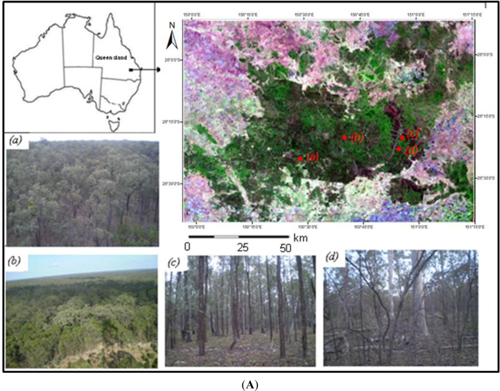
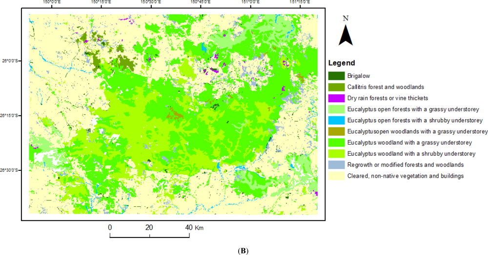
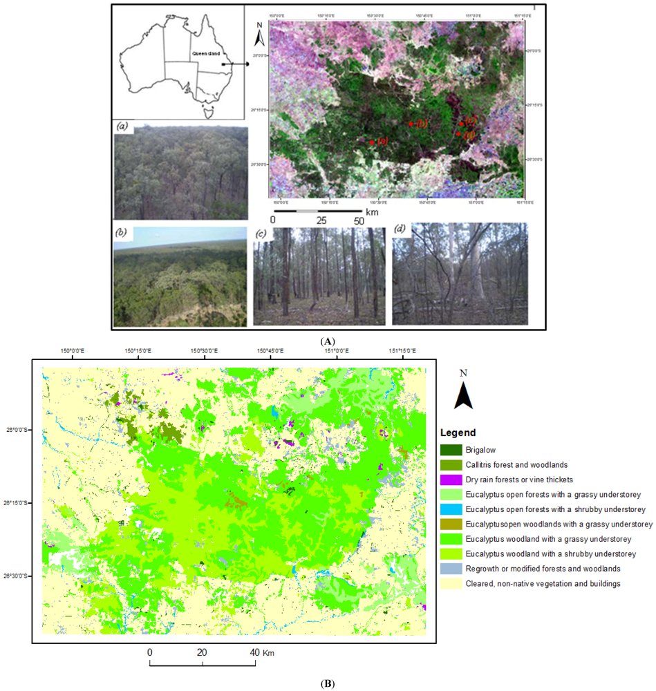
The study area is comprised of a part of Landsat TM scene WRS-2, Path 91/Row 78, located in Queensland, Australia. The major part of the area is covered by Barakula state forest, which is the largest state forest in Australia. The forests lies in the Brigalow Belt bioregion and covers an area of 260,000 ha (Figure 1). The forests are dominated by mature eucalypt and cypress pine woodlands and open forests. The understory is either shrubs or grasses, which green up on a seasonal cycle. According to National Vegetation Information System (NVIS) dataset [26], the area has 10 major vegetation sub-groups. The non-forest area is mainly covered by agriculture, buildings and non-native vegetation. Table 1 shows the major vegetation types and the area covered by them. Topographically, the area is relatively flat and receives an average annual rainfall of 660 mm with a relatively wet summer (November–February) and dry winter (June–July).
Criteria for site selection included the availability of ground-measured foliage projective cover (FPC) data in 10 permanent measuring plots established by the Department of Environment and Resource Management (DERM) of the Queensland Government. FPC is a commonly adopted metric of vegetation cover in many vegetation classification frameworks in Australia [27]. It is defined as the vertically-projected fractional area covered by one or more layers of photosynthetic foliage of all strata in a given area [28]. The FPC is closely related with vegetation projective cover (VPC) or canopy cover as the exclusion of the fraction covered by branches and stem in VPC results in FPC. Generally, FPC makes up about 80–90% of the VPC for woody vegetation depending on canopy structure. As Australian vegetation communities are dominated by trees and shrubs with irregular crown shapes and sparse foliage, FPC is considered a more suitable indicator of a plant community’s physiological activities such as photosynthesis and transpiration than the crown cover [29].
Landsat TM images L1T product of WRS II path 091 and row 078 were used. All Landsat 5 TM scenes from 2003 to 2008 available from USGS Land Processes Distributed Active Archived Centre were acquired https://lpdaac.usgs.gov/lpdaac/get_data. A part of the scenes (140 km × 100 km), that covers the Barakula State Forest was subset and used for LITS development. MODIS collection 5 Nadir-Bidirectional Reflectance Distribution Function (BRDF) Adjusted Reflectance (NBAR) product was used as the input MODIS reflectance to the STARFM algorithm. The collection 5 MODIS NBAR (MCD43A4) is a 16 days composite product, produced in every 8 days with a quasi-rolling strategy [30]. All NBAR scenes (h31v11) of the area from July 2003 to July 2008 were acquired https://lpdaac.usgs.gov/lpdaac/get_data. MODIS reflectance was used as an input for the STARFM algorithm for gap filling purpose.
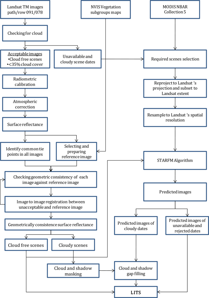
2.2. Landsat Image Time Series (LITS) Preparation
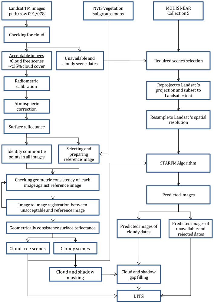
Image selection, cloud and cloud-shadow masking, geometric and radiometric correction, and gap filling were the major steps of the LITS preparation. Figure 2 summarizes the steps of the LITS preparation.
2.2.1. Image Selection
The main purpose of image selection was to identify the images suitable to use for the LITS development over the period of five years from July 2003. An image with some cloud cover could be used in LITS after masking cloud and cloud shadow and filling the gaps created. An image with few uncontaminated pixels could also be replaced by a predicted image instead. Images with more than 50% unusable pixels due to cloud and cloud shadow were discarded from analysis. A close evaluation of all cloudy images revealed that an average of 35% cloud cover would make about 50% of the data contaminated with the combined effects of cloud and cloud shadow. The available images were categorized by visual evaluation as cloud-free scenes that can be used directly in the LITS and also as an input to the STARFM algorithm to predict the synthetic images to fill gaps, and cloudy scenes with less than 35% cloud cover, which can form part of the LITS after masking clouds and filling the gaps as outlined earlier. In total, 75 usable scenes were found for the period, out of which 38 were cloud free.
2.2.2. Cloud and Cloud-Shadow Masking
Masking cloud and cloud shadow was critical to develop the LITS. The pixels contaminated with cloud and shadow generally have sufficiently different reflectance properties than the actual land cover and produce erroneous information if used in an automated mapping algorithm [31]. Manual cloud masking was assisted by identifying pixels which appeared brighter than usual when compared over time. A python script was used to identify and mask the unusually brighter pixels and the identified areas were then manually edited where needed. Cloud shadows were masked using manual digitizing.
2.2.3. Radiometric Calibration and Atmospheric Correction
All images were converted to surface reflectance for two reasons. Firstly, it would make the images in the LITS comparable through time and ready to use for deriving biophysical variables of interest [32,33]. Secondly, only the surface reflectance can be used as an input to the STARFM algorithm to predict the Landsat images for gap filling [17].
The Landsat 5 TM L1T images were first converted to top of the atmosphere (TOA) radiance using standard equations and calibration parameters obtained from the metadata of each scene [34,35]. The TOA radiance was used to compute the surface reflectance using 6S radiative modeling code [36]. The atmospheric parameters needed for the code were ozone concentration, column water vapor and aerosol optical depth (AOD) at 550 nm [36]. The ozone concentration was derived from total ozone mapping spectrometer (TOMS) climatology data [37]. The column water vapor was derived from daily interpolation of point observations of vapor pressure [38]. A continental model for describing the aerosol proportions was used (dust-like = 0.7, water soluble = 0.29, oceanic = 0, soot = 0.01).
A fixed value for AOD was used as it is difficult to get AOD values over the site. There is no field instrumentation, and image-data estimates, such as those from the MODIS and the Multi-angle Imaging SpectroRadiometer (MISR), are rarely available coincident with the image acquisitions. The dense dark vegetation method [39] can potentially be used to retrieve AOD directly from the imagery, but there are limitations in applying this method in Australia as the spectral-reflectance of the vegetation is neither sufficiently dark nor temporally-invariant [40]. In addition, the root mean square error of different AOD retrieval algorithms from satellite data shows that they are not sensitive enough to accurately predict low AOD values [41,42], which are typical of Australia’s atmosphere. The value of 0.05 was chosen as available aerosol robotic network (AERONET) sun-photometer data over the Australian continent showed that AOD remains under 0.1 in most of the cases http://aeronet.gsfc.nasa.gov/cgi-bin/bamgomas_interactive. For example, about 80% of the AERONET data from Birdsville, Southwest Queensland were less than 0.1 [43].
2.2.4. Geometric Correction and Validation
The L1T product of Landsat TM images are corrected for geometric accuracy using ground control points and digital elevation model (DEM). The accuracy depends on the quality of the control points and the resolution of the DEM used. The images are required to be geometrically correct with sub-pixel accuracy for the LITS to be suitable for temporal comparison. A common point comparison (CPC) method was used to ensure all images are geometrically correct and precisely registered to each other. An image was first prepared as a reference to examine the geometric consistency of the whole time series. The image of 2006/02/01 was chosen as a reference as it was cloud free and near the mid-point of the time series. The geometric accuracy of the reference image was ensured using image to map registration using vegetation subgroup map. To avoid the resampling of the images, the reference map was first projected to the same projection as the images obtained from the USGS.
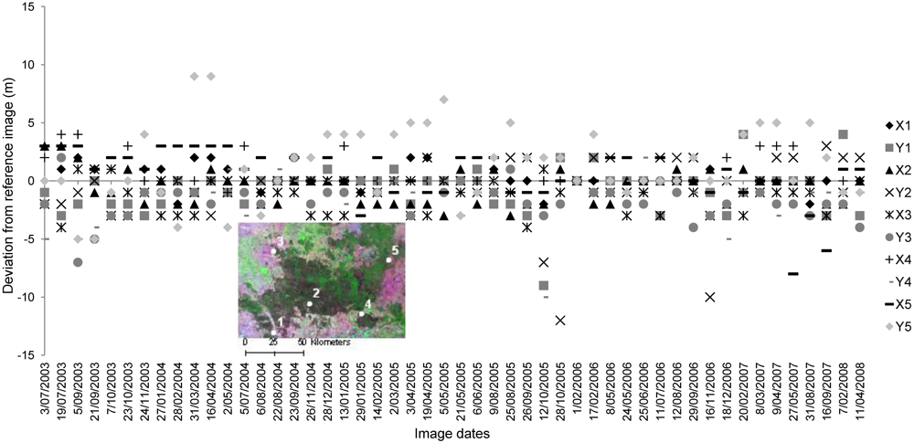
Five well-distributed points within the image subset (Figure 3) were identified as common tie points in reference image. Care was taken to select the points so that they could be easily located in all images and were cloud free in most of the scenes. Those tie points were identified manually in all images and a list of X and Y coordinates of the points was created. The deviations of the coordinates of all images from reference image in both the X and Y directions were calculated. A threshold of 15 m (half a pixel) was chosen and all images with a registration error more than the threshold value with reference image in either direction were identified. All identified images were then corrected using image to image registration method with the reference image to achieve a registration error of less than 15 m.
2.2.5. Creating Synthetic Landsat Images using the STARFM Algorithm and Assembling the LITS
The STARFM algorithm predicts reflectance at the Landsat TM’s spatial resolution using one or more pairs of Landsat TM and MODIS images acquired on the same date and MODIS reflectance from the date at which the Landsat TM reflectance is to be predicted [17]. STARFM predicts Landsat TM pixel values based on a spatially weighted difference computed from a selected moving window between input Landsat TM and MODIS images of date one, T1, and the temporal difference between MODIS images of T1 and T2 (prediction date) [17]. The theoretical basis, assumptions and other details of the prediction algorithm can be found in Gao et al. [17] and Hilker et al. [24]. The STARFM algorithm written by Gao et al. [17], which was capable of predicting each Landsat band at a time was received and used for this study.
Careful selection and preparation of Landsat TM and MODIS scenes was required. To predict all six reflective Landsat TM bands, reflectance products with 500 m spatial resolution could only be used as all corresponding MODIS bands with Landsat TM-like wavelength were not available at the 250 m spatial-resolution. The MODIS nadir-view BRDF-adjusted reflectance (NBAR), MCD43A4, product was used as it offers additional benefits to a standard reflectance product. As MODIS reflectance may still contain significant variations due to viewing geometry [44], the NBAR product with nadir viewing geometry is similar to Landsat TM’s viewing geometry. MODIS NBAR is a Terra and Aqua combined product modeled from the BRDF model parameters (product MCD43A1) to provide reflectance as if they were taken from nadir view [45].
All bands with equivalent bandwidth to Landsat’s reflective bands as shown in Table 2 of MODIS NBAR imagery were re-projected and subset using GDAL Utilities tools http://www.gdal.org/gdal_utilities.html to match the Landsat TM image extent for Barakula Forest. They were resampled to 30 m spatial resolution using GDAL translate tool. Nearest neighbor resampling approach was used as does not alter the reflectance value. In addition to having similar spatial resolution and projection, the data format of Landsat TM and MODIS imagery were also required to be same format for data fusion. The Landsat TM images, therefore, were also stored in 16 bit format. GDAL translate tool and Python programming language were used to accomplish the tasks.
The STARFM algorithm was run for all dates, when Landsat TM images were either cloudy or unavailable. Though STARFM can work on single-pair inputs, the prediction quality improves when two pairs of Landsat TM and MODIS images acquired on the same date are used as input [17]. It is not only the number of input pairs; the acquisition date of those images also affects the results [19]. A balance between number of input pairs and the time difference between the acquisition date of those data and prediction date was desirable. It was therefore decided to use two pairs of inputs only if they were available within two months either side of the prediction date. As the MODIS images were 16-day composites, it was not possible to have the MODIS images exactly matched to the Landsat TM dates. To address this, MODIS images of the closest date prior to the Landsat TM acquisition were used.
The LITS was assembled using all cloud-free original scenes and STARFM predicted synthetic Landsat TM images. Synthetic imagery for those dates in which Landsat TM images were either unavailable or rejected due to high cloud cover were directly included in the LITS. For other dates when less than 50% of the original data were contaminated, the synthetic images predicted were used to fill the gap of the cloud and cloud shadow, and gap filled images were included in the LITS.
2.3. Evaluation of the LITS
The LITS was evaluated in two steps. First, the accuracy of STARFM predicted synthetic imagery was assessed. The accuracy as a time series was assessed in the second step. Synthetic Landsat TM images were generated for three dates (Table 3) for which a good quality original Landsat TM images were available and used for comparison.
2.3.1. Accuracy of Predicted Landsat TM Images
The accuracy of STARFM predicted synthetic imagery was assessed by two means. Firstly, direct reflectance comparison was carried out between original and predicted images. The prediction accuracy was assessed on a pixel by pixel basis by means of correlation between the reflectance of original images and predicted images. The reflectance between original and predicted images was also compared for major vegetation communities in the study area to see if the prediction accuracy was different within different structural forms of vegetation. The mean and standard deviations of at-surface reflectance for all major vegetation communities were calculated from both the original and predicted images and compared. StarSpan [46] was used to extract the mean and standard deviation of reflectance value from all pixels with in the vegetation communities.
Secondly, FPC values derived from predicted images were compared with ground measured values. FPC values measured in 2005/07/11–13 at ten different field plots of 100 m diameter were available. The details of the method used to measure FPC in the field can be found in Armston et al. [47]. FPC values were derived from two predicted images of 2005/07/08 and 2005/07/24, which were the closest images before and after the field measurement. A multiple linear regression method was used to derive FPC from those images, using the reflectance of all reflective bands as explanatory variables. As field measured values within the study area were not sufficient to build a regression model, FPC maps of the area dated 2003/09/05, 2006/07/11 and 2007/02/04 developed by DERM were used as reference data sets to build the regression model. FPC maps used as reference data in this study were produced by DERM from Landsat images as a part of their state-wide vegetation monitoring program. Those maps were produced using a multiple regression model developed from an intensive field measured dataset of approximately 1,400 sites representing all types of vegetation communities and environments across the state of Queensland [47]. The regression model developed by DERM was not directly applicable to produce FPC maps from the images used in this study as the radiometric and atmospheric correction routine applied were different from those images used by DERM. Therefore, a separate regression model was developed from those FPC maps and reflectance values of all reflective bands from the corresponding pixels of Landsat TM images of the same dates. The pixels were selected systematically using a grid of 1000 m and 80% of the selected pixels were used to calibrate the regression model. The remaining 20% pixel values were used as to validate the model and an R2 of 0.88 was achieved. The model then used to produce FPC maps from the LITS. As the field measured values were from plots of 100 m diameter, an average FPC value of 3 × 3 pixels in the images of 2005/07/08 and 2005/07/24 were extracted for those plots and compared with the ground-measured values. Coefficients of determination (R2) and root mean square error (RMSE) terms were calculated to examine accuracy level. The linearity assumption of multiple regression was checked to verify whether it violated the assumption.
2.3.2. Accuracy of the Time Series
The accuracy of the predicted images was an important component of the LITS accuracy but that alone may not signify its overall usefulness. The usefulness of the LITS depends on how accurately the LITS generated time series represents actual changes in vegetation and other properties on the ground. Therefore, the second part of the evaluation assessed the accuracy of the time series generated from the LITS representing a particular location or a vegetation community. As there was no direct means of assessing the accuracy of the LITS-generated time series, several indirect methods were used. Firstly, NDVI images were generated from the LITS and the mean and the standard deviation of NDVI values of all images in the time series were calculated for all vegetation communities using StarSpan [46]. The calculated mean and standard deviation of NDVI values from all original and predicted images were plotted in a time series plot and visually evaluated to determine the extent to which the predicted images followed a pattern of the original.
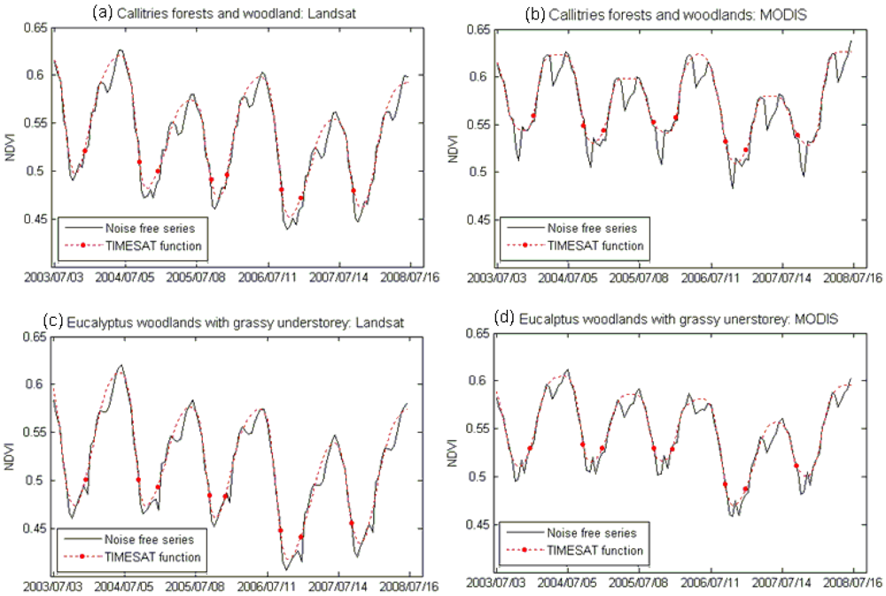
Secondly, NDVI time series generated from the LITS were compared with MODIS NDVI time series, generated from the MOD13Q1 product, to assess their similarities and differences in terms of their overall shape and their ability to capture information on vegetation phenology. Comparison with MODIS NDVI values was carried out as they are considered the best available scientific data ready to use for vegetation monitoring and represent vegetation phenology correctly [25,48]. Trend and seasonal components, were decoupled using Seasonal Trend Decomposition based on Locally weighted regression (STL) algorithm [49] and examined for different forest communities. The series were decoupled using R and a seasonal window of 35 and frequency of 23 was used as input parameters. A Mann-Kendall Trend Test was used to test the difference the trend extracted from LITS and MODIS NDVI time series. Similarly, quantitative seasonal parameters including the start, end and peak dates of the growing season were calculated from both Landsat TM and MODIS time series using the TIMESAT 3.0 program [50]. The parameters were calculated from noise free Landsat TM and MODIS NDVI time series removing the error components shown by the STL algorithm from the original series and compared for different forest communities.
3. Results
3.1. Geometric Consistency of the LITS
Figure 3 shows the geometric consistency among the images used to develop the LITS. It shows the registration accuracy of all images with a common reference image of 2006/02/01. The different symbols on the graph show the difference in X or Y coordinates at the five points of a particular image compared to the reference image. It can be seen that an average registration error of less than 10 m (one third of a pixel size) in most of the cases and less than 15 m in all cases was achieved. The images which are not shown in the figure due to the missing values of one or more tie points due to cloud cover had the same range of error values in available points. As the registration accuracy of the predicted images remains similar to the input Landsat TM images, the registration error of all images in the LITS was considered to be within a half of a Landsat TM pixel in each dimension.
It was found during the CPC procedure that the registration accuracy of the USGS supplied L1T TM images was acceptable in most of the cases. No images with registration error more than 30 m in one dimension were observed. About 80% of the examined images in this case were within acceptable registration accuracy and no treatment was required. Only remaining 20% of images had the error more than selected threshold of 15 m, and image to image registration to the reference image was required.
3.2. Accuracy of the STARFM Generated Landsat TM Imagery
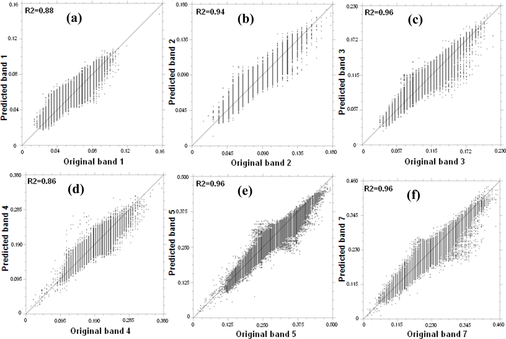
Table 3 shows the description of three predicted Landsat TM images used for assessing the prediction accuracy of the STARFM algorithm. The prediction dates were chosen so that the original Landsat TM images for all three dates as well as all other required input images were cloud free and good quality. Figure 4(a–f) shows per-pixel comparison of reflectance from all six reflective bands of the original Landsat TM image of 2006/06/25 and the predicted image. It shows the fit of scatter plots to the 1:1 line and the coefficient of determination (R2) values.
The distribution of the scatter plots around the 1:1 line and the consistently high correlation (R2 > 0.85) values across all bands (Figure 4(a–f)) showed that the predicted image was able to explain most of the variation in the original image in this case. The mean R2 value between original and predicted images of all three dates 0.61, 0.78, 0.86, 0.81, 0.90, 0.90 for Landsat bands 1, 2, 3, 4, 5 and 7 respectively showed that STARFM maintained a reasonably accurate predicting capability in this environment. The R2 values across the different vegetation communities (Table 4) in the study area showed a similar trend with some exceptions in bands 1 and 2. In general a higher accuracy was observed in longer wavelength bands. The possible reasons of such exception follow in Section 4.2.
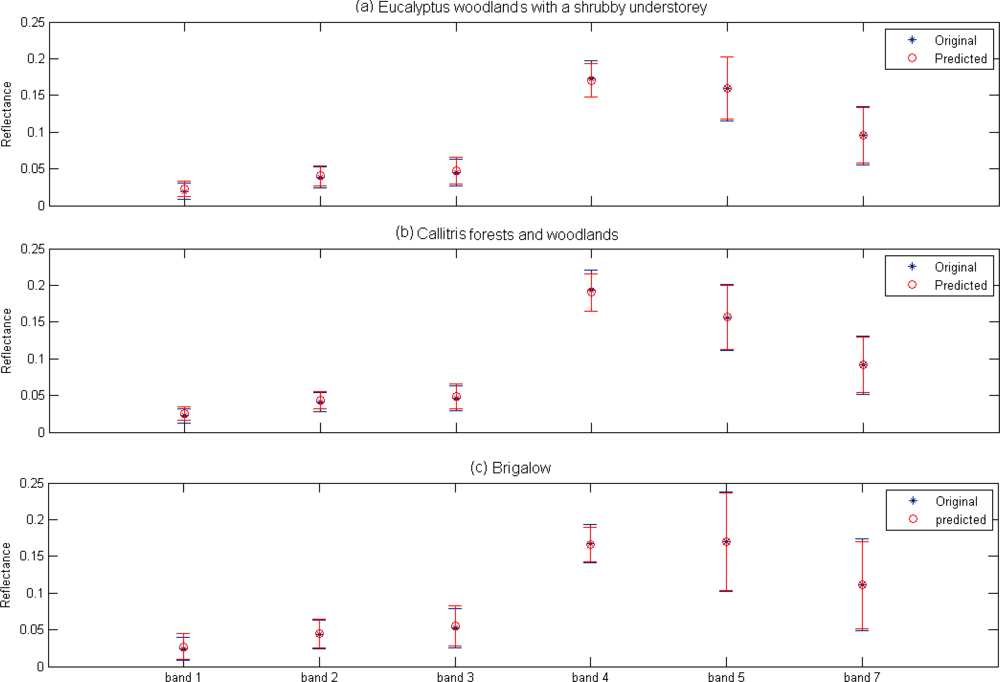
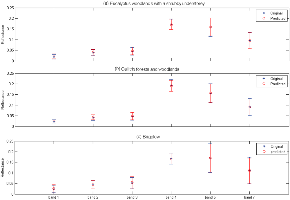
Figure 5(a–c) shows an example of a quantitative comparison of reflectance between the original Landsat TM reflectance values and those in the predicted image for 2006/06/25 for three different vegetation communities in all bands. The predicted reflectance was higher in visible bands (1–3) and smaller in infrared bands (4, 5 and 7) than the original. The difference was bigger in lower bands with highest positive difference in band 1-blue and lowest in band 3-red and highest negative difference in band 4—infrared and lowest in band 7—short-wave infrared. Among them, the highest absolute difference in mean and standard deviation between original and predicted reflectance values was in band 1—blue. Eucalyptus woodland with shrubby understory showed the highest difference of 16% from the original image in mean and Brigalow showed the highest difference of 19% from the original image in standard deviation. The lowest difference was in band 5 middle infra-red (0.21% in mean and 1.96% in standard deviation in Callitris forest and woodland and Brigalow respectively). The average of all vegetation communities showed that the highest difference both in mean and standard deviation between the reflectance of the original and predicted images was in blue band (12.95% in mean and 18.48% in standard deviation) and the lowest difference of 0.14% and 10.45% in band 7 (short-wave infrared).
The difference in mean and standard deviation observed between the original and predicted Landsat TM reflectance images, however, was statistically significant. A two sided t-test with α = 0.05 showed that the mean predicted reflectance for different vegetation communities across all bands were not statistically similar to the mean of the original reflectance in most cases.
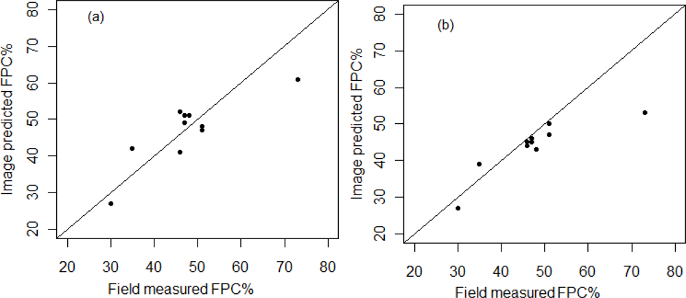
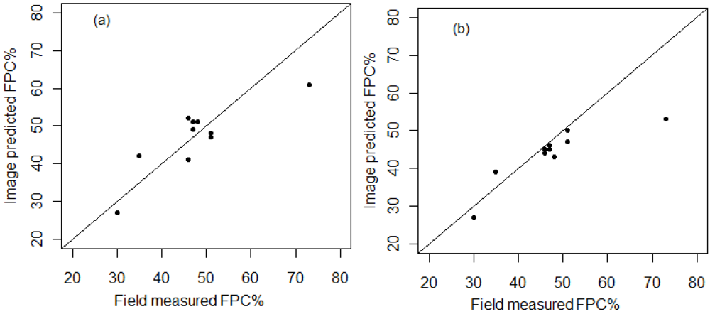
Figure 6(a,b) shows the accuracy of the FPC map derived from STARFM predicted images by comparing the FPC values measured in ten different plots in 2005/07/11–13 with image-derived FPC. The accuracy was reasonably good with a R2 of 0.73 and root mean square (RMSE) of 5.6 for 2005/07/08 image and a R2 of 0.75 and RMSE of 6.9 for 2005/07/24 image. The accuracy in 9 out of 10 plots was better as the RMSE was only 4.38 for 2005/07/08 image and 2.92 for 2005/07/04 image excluding a plot in Brigalow forests with high FPC value. The higher error in the areas with higher ground-measured FPC was also observed by Armston et al. [47], and reported that the regression based approach was less accurate when estimating image-derived FPC for forested areas with more than 50% FPC.
3.3. Ability of the LITS to Capture Vegetation Phenology
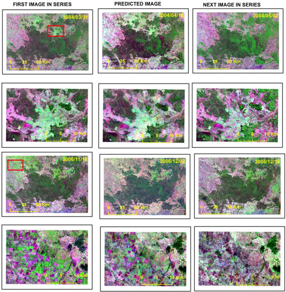
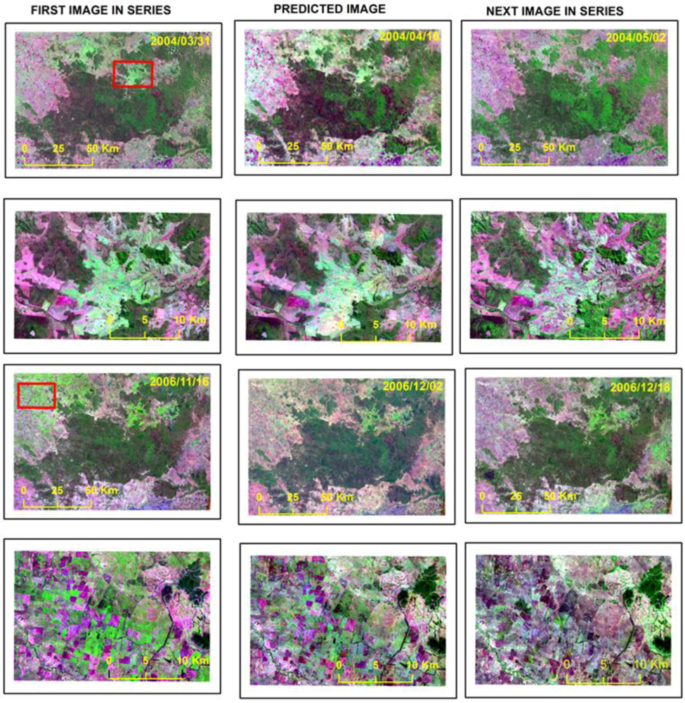
The ability of the LITS to capture vegetation phenology was assessed by examining images visually and comparing means and standard deviations of the original and predicted images in the LITS. Figure 7 shows the images from two subsets of the LITS in band combination 5, 4 and 3 as red, green and blue. Each subset features two Landsat TM images and a predicted image in the time period in-between the original images. The decreasing seasonally-green area between the two original images has been captured by the predicted images in the middle of the time series. The second and last row of the figure, a zoomed out area from the earlier rows shows that the predicted Landsat TM images are showing a scenario between the two original images, demonstrating the ability of LITS to capture the vegetation phenology.
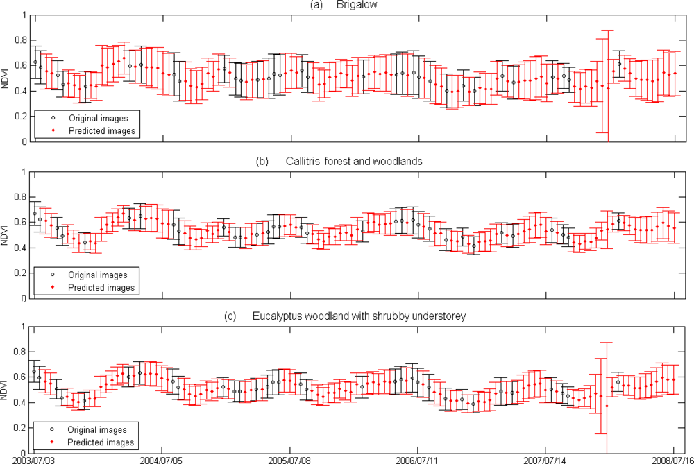
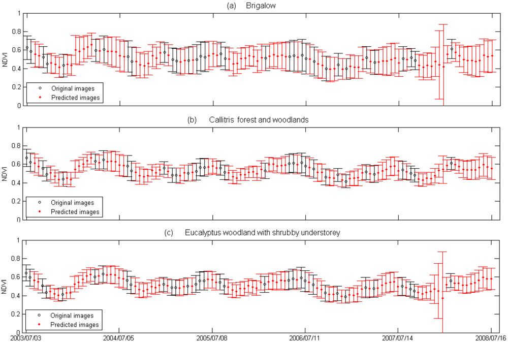
An evaluation of the mean and standard deviation of NDVI for different vegetation communities also showed that the LITS was able to capture the seasonal change in vegetation. Figure 8(a–c) shows a time series plot of means and standard deviations of NDVI value of all images in the LITS for three different vegetation communities. It can be observed from the figure that the mean and standard deviation of NDVI value of the predicted images follow the seasonal pattern shown by the mean and standard deviation of NDVI value of the original images. It also showed that the standard deviations of all predicted images except from the images of 2007/12/21 and 2008/01/06 were similar to the original images and therefore had followed the seasonal pattern of the original. The possible reasons of the high standard deviation for those days follow in discussion (Section 4.2).
3.4. Comparing LITS and MODIS NDVI Time Series
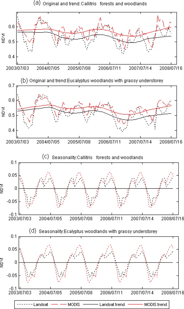
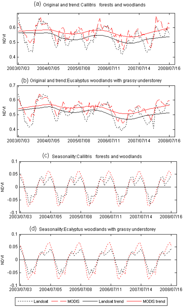
The averaged NDVI time series generated from the LITS for different forest communities in Barakula State Forest were compared to the respective MODIS NDVI time series of the same period. As the Landsat TM acquisition dates don’t exactly match with MODIS 16 day composite product dates, MODIS NDVI of nearest earlier date from Landsat TM dates were considered to be equivalent for the comparison. Figure 9(a–d) shows the Landsat TM and MODIS NDVI time series for two vegetation communities of Callitris forests and woodlands and Eucalyptus woodlands with grassy understorey. Figure 9 compares the original NDVI time series along with the trend and seasonal components. The visual comparison of the original time series showed a level of similarity in overall shape between them, but the NDVI time series from MODIS were found higher than NDVI time series generated from LITS.
The comparison of trend and seasonal components could be more useful than the comparison of the original series as they signify whether the NDVI time series generated from the LITS are showing similar pattern of vegetation change as shown by MODIS time series. The visual comparison of time series plots reveals that there is a slight difference between trends and seasonal components of the LITS and MODIS NDVI time series. A Mann-Kendall test, however, showed no significant difference between the trends of MODIS and Landsat TM time series for both vegetation communities. The test showed that the trends were slightly negative in all cases but none of them were significant at α = 0.05 (τ = −0.094, two sided p = 0.13 for Landsat TM time series and τ = −0.05, two sided p = 0.37 for MODIS time series of Callitris forests and woodlands and τ = −0.097, two sided p = 0.12 for Landsat TM time series and τ = −0.08, two sided p = 0.17 for MODIS time series of Eucalyptus woodlands with grassy understorey).
The quantitative evaluation of seasonality shown by two different series was performed using the key seasonal parameters: start, end and peak time of a growing season. Figure 10(a–d) shows the logistic polynomials fitted by the TIMESAT program [50] to produce the information. The information on start-point, end-point and peak time of a growing season was extracted for four seasons as shown by dots in the fitted polynomials in Figure 10(a–d). The Landsat TM data generally showed an earlier start and a longer growing season compared to MODIS, but the difference was reasonably small considering the 16 days composite period for MODIS NDVI and similar nature of MODIS reflectance used to predict Landsat TM images. The average difference in the start of the seasons between Landsat TM and MODIS NDVI series was 21 days for Callitris forest and woodlands. The average difference in end of season and peak timing were 3 and 12 days, respectively. In the case of Eucalyptus woodlands with grassy understorey the average difference in start, end and peak of season were only 10, 5 and 4 days respectively. The comparison for other vegetation communities also showed that the difference between key seasonal parameters shown by two different series was less than 16 days in eight out of 10 vegetation communities.
4. Discussion
This study tested the STARFM algorithm in a Eucalyptus woodlands environment and also showed the usefulness of the algorithm to build a long and regular time series of Landsat TM images capable of capturing vegetation phenology. The pre-processing routine applied to Landsat TM images was able to derive surface reflectance for input to the STARFM algorithm [17]. Altogether 77 synthetic Landsat TM images were produced using 38 cloud-free Landsat TM images and 115 MODIS NBAR images for the period between 2003/07/03 and 2008/07/16 to build the regular time series by filling the gaps due to clouds. The methods and data used produced an LITS with an observation every 16 days.
4.1. Preparing Landsat Thematic Mapper Images and Choice of MODIS Data Sets
Atmospheric correction of Landsat TM images is still an issue for operational implementation [18] due to the difficulties of acquiring all of atmospheric parameters required at the time of the overpass. The atmospheric correction routine applied in this study assumed that the AOD at 550 nm in the study area remained 0.05. Published reports [43,51] and the data available from AERONET ( http://aeronet.gsfc.nasa.gov/) webpage for different sites in Australia showed that it is reasonable to assume an AOD of 0.05 in most of the areas in Australia except the Northern tropics. The almost similar prediction accuracy of September and June images (Table 4) also indicated that the assumption of a fixed AOD of 0.05 was appropriate in this context. AERONET AOD data showed that the atmosphere in June was near its clearest with low AOD values, while in September it was at it had very low visibility and high AOD, due to smoke from fires. Assuming constant AOD is a limitation of the approach used in this study and may limit the approach in areas of temporally and spatially variable AOD.
The use of the MODIS NBAR product instead of the daily or 8-day composite MODIS reflectance as the input MODIS dataset to STARTFM was useful for two reasons. Firstly, the use of a composite product like NBAR enables prediction of the Landsat TM reflectance even in areas where cloud cover prohibits acquisition of frequent cloud free images [24]. Except for the two MODIS scenes used to predict the December 2007 images, all other scenes used in this study were free from missing data due to cloud cover and helped to predict Landsat TM scenes correctly to complete the LITS. Secondly, compared to the daily or 8-day composite MODIS reflectance, the viewing and illumination geometry of the NBAR product is similar to the Landsat TM images. The daily MODIS reflectance product can have a significant reflectance variation, particularly on the edges of the images due to its wide (±55°) sensor view angle compared to ±7°of Landsat. The 8 day or 16 day composite products are meant to be from near nadir viewing observations but in practice about 50% observations could be from high viewing angles (>20°) as observed in an analysis of 34 randomly selected pixels of MOD13Q1 in the study area from 161 scenes (2001–2007) [52]. As the solar geometry remains more or less similar between Landsat TM and MODIS, the use of NBAR product reduces the differences in viewing geometry over most of the Landsat TM scenes. The use of NBAR data, however, may impact the accuracy of predicted reflectance as the NBAR product represents an averaged scenario for a 16-day composite period, rather than the actual Landsat TM date of prediction. The NBAR product may not be available for all required dates as missing data was encountered here for two dates. The problem could be more serious in tropical regions where more frequent cloud cover and smoke contamination exists. Use of quality checking and temporal interpolation tools like TiSeG [53] can help to get the data for all required dates but will also increase the uncertainty of prediction as interpolated values may not truly represent the actual values.
4.2. Accuracy of STARFM Predicted Images and the LITS
The accuracy of predicted images observed in this study showed the STARFM algorithm [17] worked well in a eucalyptus-dominated broad-leaved forest environment, similar results to Hilker et al. [24] from coniferous forests. The very low R2 value (0.08) of Dry Rain Forests on 2006/06/25 images was the result of missing blue-band data over the area in the input MODIS image. No obvious reasons were determined for the other low values of 0.20 for Eucalyptus Open Forests with grassy understorey on 2003/09/05, 0.41 for Eucalyptus Open Woodland with grassy understorey on 25 June 2006 and 0.30 for dry rain forests on 2007/06/30 for band 1 and 0.44 for Dry Rain Forests on same date for band 2. Higher prediction accuracy in the infrared bands than the visible bands as observed in this case was also reported by Hilker et al. [24] in coniferous forest environments. The reason for the difference is likely to be due to the separate atmospheric correction routines applied for Landsat and MODIS reflectance. The difference in atmospheric conditions at the time of image acquisition for input MODIS image and original Landsat TM image could also be the reason for the poor relationship for blue bands. The reason is that the shorter wavelengths are more affected by atmospheric attenuation than the longer wavelength [18].
The significant difference between the reflectance of original and predicted images for different vegetation communities observed in this study was different from the earlier study of Hilker et al. [24], who reported no significant difference in original and predicted reflectance. The important question was whether the difference is important for further image analysis tasks as the difference in mean does not always have the same effect. For example, if all reflectance values in different bands are offset in one direction proportionately, no impact may be observed in the analysis results though the offset image may have a significantly different mean value from the original. However, if the difference in means was due to a random change in values, it could affect the analysis results. The change in standard deviation and the per-pixel correlation, therefore, could be a stronger measurement of the similarity and differences in images in terms of output products. As the correlation observed in this case was significant, the difference in standard deviation was small between original and predicted images in most of the bands, the images could still be useful to monitor vegetation change. The accuracy of the FPC product derived from the predicted images (Figure 6(a,b)) indicated the usefulness of the approach to develop a time series of FPC to monitor change in structural properties of vegetation over time. As the result shown here was based on only 10 field plots, testing the approach in other areas where more field-measured FPC values are available will signify whether the approach can be used operationally to develop FPC time series in Queensland.
The other difference observed in this study was a smaller prediction accuracy (R2 value) for band 4 (near-infrared) than band 3 (red), an exception of the trend of higher accuracy for long wavelength bands reported in an earlier study and observed in this case. The correlation observed in this study for band 4, however, was not smaller than that reported by Hilker et al. [24] but the correlation for band 3 observed here was higher. Similarly, the positive prediction error at visible bands and negative prediction error in infrared bands observed in this study was also interesting. The reason for this could be the difference in vegetation canopy, branch and trunk structure between coniferous and broadleaf forests, which results in different BRDF properties at the Landsat and MODIS scales.
The pattern of means and standard deviations of predicted and original images (Figure 8(a–c)) indicated the usefulness of STARFM generated images as a part of long time series. Examination of the input MODIS data showed that the abnormally high standard deviation of two dates (2007/12/12 and 2008/01/06) was the result of missing data in the input MODIS imagery used for prediction. For example, about 40% of pixels covering the area were missing in the MODIS NBAR imagery dated 2007/12/19 and input MODIS image for prediction of Landsat image dated 2007/12/21. The Callitries forests and woodland were not affected as the MODIS data for that area were not missing. Quantitative analysis also showed that the difference in standard deviations of NDVI between original and predicted images excluding those exception images was small. For example, the absolute difference between averaged standard deviation of original and predicted images for Briglow, Callitries forests and woodlands and Eucalyptus woodlands with shrubby understorey was 1.15%, 4.09% and 3.63% of the average value of original images respectively.
The similarities in the overall trend of the NDVI time-series derived from the LITS with the NDVI time series extracted from MODIS product (Figures 9(a–d) and 10(a–d)) also indicated the usefulness of the STARFM algorithm to produce a long and regular time series which can be used to study vegetation phenology. However, the MODIS NDVI series were higher than the LITS generated NDVI series. A certain level of difference in the NDVI series is an anticipated behavior as identical NDVI values from the images with different spatial resolution and acquired by different sensors can’t be expected. The spatial point spread functions of Landsat TM and MODIS sensors are different and the simple spatial averaging cannot mimic the functions and won’t produce the similar values [20]. In addition, the gridding effects of MODIS reflectance [54] could also have some negative effect. Besides, the higher red reflectance in band 3-red and lower infrared reflectance in band 4—infrared in predicted images also contributed to lower the NDVI series generated from LITS. In spite of the difference, as both series showed similar trend information and coincident key phenological metrics, like start of season and end of season, were smaller than the composite period of the MODIS data (16 days), the LITS can be considered capable of capturing vegetation phenology and trend in the environment and data studied in this work. The performance of LITS at individual Landsat TM pixel level, however, could not be examined due to the lack of ground-based phenological and trend information. Future studies similar to Liang et al. [25] with field information at Landsat TM spatial scale would help to assess the LITS approach with greater confidence across more environments.
The capability for detecting change in vegetation structure and condition in the predicted Landsat TM image depends on the ability of the input MODIS images to detect such change and the nature of the land cover [17]. If the two input MODIS images are captured at significant times apart, and are unable to capture the temporal change in reflectance, the predicted Landsat TM image will also be unable to record the change. In a heterogeneous landscape where similar Landsat TM pixels can’t be found within the MODIS pixel boundary, the prediction accuracy of the STARFM algorithm degrades [17,19]. The ESTARFM algorithm [19] is aimed at improving the prediction in a heterogeneous environment, but needs at least two sets of input Landsat and MODIS images as stated earlier. The ESTARFM was not used in this study as two near-date Landsat images were not available for all prediction dates. Although ESTARFM could have been used for the dates where two pairs of Landsat and MODIS image were available, STARFM was used to make all prediction in the LITS consistent.
The choice of input Landsat TM and MODIS pairs is important as the performance of these algorithms not only increases with more input Landsat and MODIS image pairs but also depends on the time difference between input images and predicted images [17,19]. Hilker et al. [55] have developed a new algorithm called Spatial Temporal Adaptive Algorithm for Reflectance Change (STAARCH) which identifies optimal input Landsat images for STARFM particularly to record major disturbances in predicted images. As the balance of the number of input image pairs and the time difference between input images and predicted images is important for the accuracy of predicted images, further tests on the impact of the number of input image pairs and the time difference of input images and predicted image are required. This information will also help to decide whether to use STARFM or ESTARFM based on the available Landsat and MODIS images for input.
5. Conclusions and Future Works
The method outlined in this paper can be used to develop Landsat Image Time Series (LITS), a relatively long, dense and regular (in time) sequence of Landsat TM/ETM+ images, suitable to be analyzed by means of time series analysis techniques, to monitor and measure seasonality and trends in the structural and physiological properties of vegetation. The STARFM algorithm performed equally well to predict the synthetic Landsat TM images in a eucalyptus dominated forest and woodlands environment compared to coniferous environments reported by earlier studies. The MODIS NBAR data set is a viable alternative to the MODIS daily and 8-day composite reflectance used in similar studies, for input to the STARFM algorithm. Moreover, the accuracy of FPC values derived from STARFM predicted images indicated that the information could also be accurate at the Landsat TM spatial scale. Future studies with sufficient ground-measured phenological data at the Landsat TM spatial scale will be required to strengthen this conclusion. The method, however, required considerable human machine interaction for the cloud and cloud shadow masking and to make sure that all images in LITS are well registered each other, it could not be fully automated.
The LITS constructed by this method can be used to derive similar phenological information compared to MODIS NDVI (MOD13Q1) time series at the vegetation-community scale in an Australian ecosystem. As MOD13Q1 NDVI also has some issues as a time series data sets due to variable viewing and illumination geometry across time [44], the LITS constructed by this method is not also free from the effect. The view zenith angle variation may not be significant in LITS due to the small scan (±7°) angle of Landsat TM but an equally important effect of solar zenith angle variation as it was observed in MOD13Q1 dataset can be expected. The satellite observations available at present, however, do not allow modelling the BRDF properties at Landsat TM spatial scale and therefore is not possible to decouple the effect of solar zenith angle variation. With ever improving technology, it can be expected that future satellite programs will make it possible to model the BRDF in Landsat-like spatial scale (e.g., through Europe’s Sentinel program or Landsat 8’s sensor) and the earth observing community will be able to model biophysical parameters more accurately at Landsat like spatial scale too.
Acknowledgments
This work is part of a PhD project funded by AusAID, Australian Government, Canberra. Reference data were received from Remote Sensing Centre of Queensland Department of Environment and Resource Management (DERM). The cloud masking task was assisted by Robert Denham of DERM. The comments from three anonymous reviewers considerably helped to shape the paper in its present form.
References and Notes
- Cohen, W.B.; Goward, S.N. Landsat’s role in ecological applications of remote sensing. Bioscience 2004, 54, 535–545. [Google Scholar]
- Santillan, J.; Makinano, M.; Paringit, E. Integrated Landsat image analysis and hydrologic modeling to detect impacts of 25-year land-cover change on surface runoff in a Philippine watershed. Remote Sens 2011, 3, 1067–1087. [Google Scholar]
- Matejicek, L.; Kopackova, V. Changes in croplands as a result of large scale mining and the associated impact on food security studied using time-series Landsat images. Remote Sens 2010, 2, 1463–1480. [Google Scholar]
- Nagendra, H.; Rocchini, D.; Ghate, R.; Sharma, B.; Pareeth, S. Assessing plant diversity in a dry tropical forest: comparing the utility of Landsat and IKONOS satellite images. Remote Sens 2010, 2, 478–496. [Google Scholar]
- Coppin, P.; Jonckheere, I.; Nackaerts, K.; Muys, B.; Lambin, E. Digital change detection methods in ecosystem monitoring: A review. Int. J. Remote Sens 2004, 25, 1565–1596. [Google Scholar]
- Lu, D.; Mausel, P.; Brondi, E.; Moran, E. Change detection techniques. Int. J. Remote Sens 2004, 25, 2365–2407. [Google Scholar]
- Kennedy, R.E.; Cohen, W.B.; Schroeder, T.A. Trajectory based change detection for automated characterization of forest disturbance dynamics. Remote Sens. Environ 2007, 110, 370–386. [Google Scholar]
- Verbesselt, J.; Hyndman, R.; Newnham, G.; Culvenor, D. Detecting trend and seasonal changes in satellite image time series. Remote Sens. Environ 2010, 114, 106–115. [Google Scholar]
- Gonzalez-Sanpedro, M.C.; Le Toan, T.; Moreno, J.; Kergoat, L.; Rubio, E. Seasonal variations of leaf area index of agricultural fields retrieved from Landsat data. Remote Sens. Environ 2008, 112, 810–824. [Google Scholar]
- Lunetta, R.S.; Knight, J.F.; Ediriwickrema, J.; Lyon, J.G.; Worthy, L.D. Land-cover change detection using multi-temporal MODIS NDVI data. Remote Sens. Environ 2006, 105, 142–154. [Google Scholar]
- Maignan, F.; Breon, F.M.; Bacour, C.; Demarty, J.; Poirson, A. Interannual vegetation phenology estimates from global AVHRR measurements—Comparison with in situ data and applications. Remote Sens. Environ 2008, 112, 496–505. [Google Scholar]
- Potter, C.; Tan, P.-N.; Kumar, V.; Kucharik, C.; Klooster, S.; Genovese, V.; Cohen, W.; Healey, S. Recent history of large-scale ecosystem disturbances in North America derived from the AVHRR satellite record. Ecosystems 2005, 8, 808–824. [Google Scholar]
- Hayes, D.J.; Cohen, W.B. Spatial, spectral and temporal patterns of tropical forest cover change as observed with multiple scales of optical satellite data. Remote Sens. Environ 2007, 106, 1–16. [Google Scholar]
- Woodcock, C.E.; Allen, R.; Anderson, M.; Belward, A.; Bindschadler, R.; Cohen, W.; Gao, F.; Goward, S.N.; Helder, D.; Helmer, E.; et al. Free access to Landsat imagery. Science 2008, 320, 1011–1011. [Google Scholar]
- Ju, J.; Roy, D.P. The availability of cloud-free Landsat ETM+ data over the conterminous United States and globally. Remote Sens. Environ 2008, 112, 1196–1211. [Google Scholar]
- Huang, C.Q.; Goward, S.N.; Masek, J.G.; Gao, F.; Vermote, E.F.; Thomas, N.; Schleeweis, K.; Kennedy, R.E.; Zhu, Z.L.; Eidenshink, J.C.; Townshend, J.R.G. Development of time series stacks of Landsat images for reconstructing forest disturbance history. Int. J. Dig. Earth 2009, 2, 195–218. [Google Scholar]
- Gao, F.; Masek, J.; Schwaller, M.; Hall, F. On the blending of the Landsat and MODIS surface reflectance: predicting daily Landsat surface reflectance. IEEE Trans. Geosci. Remote Sens 2006, 44, 2207–2218. [Google Scholar]
- Roy, D.P.; Junchang, J.; Lewis, P.; Schaaf, C.; Feng, G.; Hansen, M.; Lindquist, E. Multi-temporal MODIS-Landsat data fusion for relative radiometric normalization, gap filling, and prediction of Landsat data. Remote Sens. Environ 2008, 112, 3112–3130. [Google Scholar]
- Zhu, X.; Jin, C.; Feng, G.; Xuehong, C.; Masek, J.G. An enhanced spatial and temporal adaptive reflectance fusion model for complex heterogeneous regions. Remote Sens. Environ 2010, 114, 2610–2623. [Google Scholar]
- Wolfe, R.E.; Nishihama, M.; Fleig, A.J.; Kuyper, J.A.; Roy, D.P.; Storey, J.C.; Patt, F.S. Achieving sub-pixel geolocation accuracy in support of MODIS land science. Remote Sens. Environ 2002, 83, 31–49. [Google Scholar]
- Justice, C.O.; Townshend, J.R.G.; Vermote, E.F.; Masuoka, E.; Wolfe, R.E.; Saleous, N.; Roy, D.P.; Morisette, J.T. An overview of MODIS Land data processing and product status. Remote Sens. Environ 2002, 83, 3–15. [Google Scholar]
- Pohl, C.; Van Genderen, J.L. Multisensor image fusion in remote sensing: Concepts, methods and applications. Int. J. Remote Sens 1998, 19, 823–854. [Google Scholar]
- Arai, E.; Shimabukuro, Y.E.; Pereira, G.; Vijaykumar, N.L. A multi-resolution multi-temporal technique for detecting and mapping deforestation in the Brazilian Amazon rainforest. Remote Sens 2011, 3, 1943–1956. [Google Scholar]
- Hilker, T.; Wulder, M.A.; Coops, N.C.; Seitz, N.; White, J.C.; Feng, G.; Masek, J.G.; Stenhouse, G. Generation of dense time series synthetic Landsat data through data blending with MODIS using a spatial and temporal adaptive reflectance fusion model. Remote Sens. Environ 2009, 113, 1988–1999. [Google Scholar]
- Liang, L.; Schwartz, M.D.; Fei, S. Validating satellite phenology through intensive ground observation and landscape scaling in a mixed seasonal forest. Remote Sens. Environ 2011, 115, 143–157. [Google Scholar]
- DEWR. Present Major Vegetation Subgroups - NVIS Stage 1; Version 3.1; Australian Government Department of the Environment and Water Resources: Canberra, ACT, Australia, 2005. [Google Scholar]
- Sun, D.; Hnatiuk, R.J.; Neldner, V.J. Review of vegetation classification and mapping systems undertaken by major forested land management agencies in Australia. Aust. J. Bot 1997, 45, 929–948. [Google Scholar]
- Specht, R.L. The balance between the foliage projective covers of overstorey and understorey strata in Australian vegetation. Aust. J. Ecol 1981, 6, 193–202. [Google Scholar]
- Specht, R.L. Vegetation. In The Australian Environment; Leeper, G.W., Ed.; CSIRO and Melbourne University Press: Melbourne, VIC, Australia, 1970; pp. 44–67. [Google Scholar]
- Roy, D.P.; Lewis, P.; Schaaf, C.B.; Devadiga, S.; Boschetti, L. The global impact of clouds on the production of MODIS bidirectional reflectance model-based composites for terrestrial monitoring. IEEE Geosci. Remote Sens. Lett 2006, 3, 452–456. [Google Scholar]
- Huang, C.Q.; Coward, S.N.; Masek, J.G.; Thomas, N.; Zhu, Z.L.; Vogelmann, J.E. An automated approach for reconstructing recent forest disturbance history using dense Landsat time series stacks. Remote Sens. Environ 2010, 114, 183–198. [Google Scholar]
- Green, R.O.; Pavri, B.E.; Chrien, T.G. On-orbit radiometric and spectral calibration characteristics of EO-1 hyperion derived with and underflight of AVIRIS and in situ measurements at Salar de Arizaro, Argentina. IEEE Trans. Geosci. Remote Sens 2003, 41, 1194–1203. [Google Scholar]
- Jensen, J.R. Introductory Digital Image Processing: A Remote Sensing Perspective, 3rd ed.; Pearson Education Inc.: Upper Saddle River, NJ, USA, 2005. [Google Scholar]
- NASA. Landdsat 7 Science Data User’s Hand Book; Landat Project Science Office: Greenbelt, MD, USA, 2000. [Google Scholar]
- Helder, D.L.; Markham, B.L.; Thome, K.J.; Barsi, J.A.; Chander, G.; Malla, R. Updated radiometric calibration for the Landsat-5 Thematic Mapper reflective bands. IEEE Trans. Geosci. Remote Sens 2008, 46, 3309–3325. [Google Scholar]
- Vermote, E.F.; Tanre, D.; Deuze, J.L.; Herman, M.; Morcette, J.J. Second simulation of the satellite signal in the solar spectrum, 6S: An overview. IEEE Trans. Geosci. Remote Sens 1997, 35, 675–686. [Google Scholar]
- Ziemke, J.R.; Chandra, S.; Duncan, B.N.; Froidevaux, L.; Bhartia, P.K.; Levelt, P.F.; Waters, J.W. Tropospheric ozone determined from aura OMI and MLS: Evaluation of measurements and comparison with the Global Modeling Initiative’s Chemical Transport Model. J. Geophys. Res.-Atmos 2006, 111, D19303. [Google Scholar]
- Jeffrey, S.J.; Carter, J.O.; Moodie, K.B.; Beswick, A.R. Using spatial interpolation to construct a comprehensive archive of Australian climate data. Environ. Model. Softw 2001, 16, 309–330. [Google Scholar]
- Kaufman, Y.J.; Sendra, C. Algorithm for automatic atmospheric corrections to visible and near-IR satellite imagery. Int. J. Remote Sens 1988, 9, 1357–1381. [Google Scholar]
- Gillingham, S.S.; Flood, N.; Gill, T.K.; Mitchell, R.M. Limitations of the dense dark vegetation method for aerosol retrieval under Australian conditions. Remote Sens. Lett 2012, 3, 67–76. [Google Scholar]
- Guanter, L.; Gãmez-Chova, L.; Moreno, J. Coupled retrieval of aerosol optical thickness, columnar water vapor and surface reflectance maps from ENVISAT/MERIS data over land. Remote Sens. Environ 2008, 112, 2898–2913. [Google Scholar]
- Davies, W.H.; North, P.R.J.; Grey, W.M.F.; Barnsley, M.J. Improvements in aerosol optical depth estimation using multiangle CHRIS/PROBA images. IEEE Trans. Geosci. Remote Sens 2010, 48, 18–24. [Google Scholar]
- Radhi, M.; Box, M.A.; Box, G.P.; Mitchell, R.M.; Cohen, D.D.; Stelcer, E.; Keywood, M.D. Optical, physical and chemical characteristics of Australian Desert dust aerosols: Results from a field experiment. Atmos. Chem. Phys. Discuss 2009, 9, 25085–25125. [Google Scholar]
- Bhandari, S.; Phinn, S.; Gill, T. Assessing viewing and illumination geometry effects on the MODIS vegetation index (MOD13Q1) time series: Implications for monitoring phenology and disturbances in forest communities in Queensland, Australia. Int. J. Remote Sens 2011, 32, 7513–7538. [Google Scholar]
- Schaaf, C.B.; Gao, F.; Strahler, A.H.; Lucht, W.; Li, X.; Tsang, T.; Strugnell, N.C.; Zhang, X.; Jin, Y.; Muller, J.-P.; et al. First operational BRDF, albedo nadir reflectance products from MODIS. Remote Sens. Environ 2002, 83, 135–148. [Google Scholar]
- Rueda, C.A.; Greenberg, J.A.; Ustin, S.L. StarSpan: A Tool for Fast Selective Pixel Extraction from Remotely Sensed Data; Center for Spatial Technologies and Remote Sensing (CSTARS), University of California at Davis: Davis, CA, USA, 2005. [Google Scholar]
- Armston, J.D.; Denham, R.J.; Danaher, T.J.; Scarth, P.F.; Moffiet, T.N. Prediction and validation of foliage projective cover from Landsat-5 TM and Landsat-7 ETM+ imagery. J. Appl. Remote Sens 2009, 3, 033540–033540-28. [Google Scholar]
- Huete, A.; Didan, K.; Miura, T.; Rodriguez, E.P.; Gao, X.; Ferreira, L.G. Overview of the radiometric and biophysical performance of the MODIS vegetation indices. Remote Sens. Environ 2002, 83, 195–213. [Google Scholar]
- Cleveland, R.B.; Cleveland, W.S.; McRae, J.E.; Terpenning, I. STL: A seasonal-trend decomposition procedures based on Loess. J. Off. Stat 1990, 6, 3–73. [Google Scholar]
- Jonsson, P.; Eklundh, L. TIMESAT—A program for analyzing time-series of satellite sensor data. Comput. Geosci 2004, 30, 833–845. [Google Scholar]
- Mitchell, R.M.; Campbell, S.K.; Qin, Y. Recent increase in aerosol loading over the Australian arid zone. Atmos. Chem. Phys 2010, 10, 1689–1699. [Google Scholar]
- Bhandari, S. Monitoring Forest Dynamics Using Time Series of Satellite Data in Queensland, Australia. 2011. [Google Scholar]
- Colditz, R.R.; Conrad, C.; Wehrmann, T.; Schmidt, M.; Dech, S. TiSeG: a flexible software tool for time-series generation of MODIS data utilizing the quality assessment science data set. IEEE Trans. Geosci. Remote Sens 2008, 46, 3296–3308. [Google Scholar]
- Tan, B.; Woodcock, C.E.; Hu, J.; Zhang, P.; Abdou, W.A.; Ozdogan, M.; Huang, D.; Yang, W.; Knyazikhin, Y.; Myneni, R.B. The impact of gridding artifacts on the local spatial properties of MODIS data: Implications for validation, compositing, and band-to-band registration across resolutions. Remote Sens. Environ 2006, 105, 98–114. [Google Scholar]
- Hilker, T.; Wulder, M.A.; Coops, N.C.; Linke, J.; McDermid, G.; Masek, J.G.; Gao, F.; White, J.C. A new data fusion model for high spatial- and temporal-resolution mapping of forest disturbance based on Landsat and MODIS. Remote Sens. Environ 2009, 113, 1613–1627. [Google Scholar]
Figure 1.
(A) A Landsat TM image color composite, showing bands 5, 4, and 3 as red, green and blue for November 24, 2003 and locations of dry season photographs of the study area, Barakula state forest, Queensland, Australia. Photographs are shown for Eucalyptus woodland with: (a) Eucalyptus cerebra dominated canopy; (b) mixed species canopy; (c) grassy understory, and (d) shrubby understory. Photos were taken during field work in November 2008. (B) Major vegetation subgroups in the study area as categorized by the National Vegetation Information System (NVIS) database. The map was produced from NVIS major vegetation subgroups raster version 3.1 downloaded from http://www.environment.gov.au/erin/nvis/mvg/index.html#nvis31.


Figure 2.
A flow chart of the Landsat Image Time Series (LITS) preparation method.

Figure 3.
Evaluation of geometric consistency of the images used for developing LITS by common point comparison method. Y axis shows the deviation in X and Y coordinates of five different points (shown in image) in other images compared to reference images dated 2006/02/01. The symbols X1, Y1, X2, Y2 etc. represent the deviation of respective points. Only the images that were cloud free in all five points were plotted here.

Figure 4.
Per-pixel Comparison of reflectance in original and Spatial and Temporal Adaptive Reflectance Fusion Model (STARFM) predicted image of 2006/06/25 for Landsat TM bands 1-5, and 7 (a–f). All pixels of the subset image covering the study were used.
Figure 4.
Per-pixel Comparison of reflectance in original and Spatial and Temporal Adaptive Reflectance Fusion Model (STARFM) predicted image of 2006/06/25 for Landsat TM bands 1-5, and 7 (a–f). All pixels of the subset image covering the study were used.

Figure 5.
Mean and standard deviation of the Landsat TM spectral band reflectance values for original and predicted Landsat TM image of 2006/06/25 in (a) Eucalyptus woodlands with shrubby understory (b) Callitris forests and woodlands and (c) Brigalow. Similar results were found across all vegetation communities and these three were presented as an example

Figure 6.
Comparison of predicted Landsat TM image derived foliage projective cover (FPC) of: (a) 2005/07/08; and (b) 2005/07/24 with field measured FPC from 2005/07/11–13.
Figure 6.
Comparison of predicted Landsat TM image derived foliage projective cover (FPC) of: (a) 2005/07/08; and (b) 2005/07/24 with field measured FPC from 2005/07/11–13.

Figure 7.
Comparison of predicted Landsat TM images band 5, 4 and 3 as red green and blue (central column) with original images of earlier acquisition dates (left column) and later acquisition dates (right column). The second and last row shows the zoomed out area indicated by a rectangle in the first images of the earlier rows. It shows an example of predicted image capturing seasonal change in vegetation cover.

Figure 8.
Time series of mean NDVI values derived from LITS for three different vegetation communities (a) Brigalow, (b) Callitris forests and woodlands and (c) Eucalyptus woodlands with shrubby understorey. The circles show the mean NDVI from the original images and the asterisks show the value from predicted images. The corresponding error bars show the standard deviations.

Figure 9.
Comparison of LITS generated normalized difference vegetation index (NDVI) time series with Moderate Resolution Imaging Spectroradiometer (MODIS) NDVI time series. The time series were generated averaging all pixels within the vegetation communities. The trend (a), (b) and seasonality (c), (d) shown were decoupled using the Seasonal Trend Decomposition based on Locally weighted regression (STL) algorithm.

Figure 10.
Extraction of seasonal parameters from Landsat TM and MODIS NDVI time series using the TIMESAT program. (a) and (b) Callitris forests and woodlands; (c) and (d) Eucalyptus woodlands with grassy understorey. The polynomials were fitted in noise free NDVI series using the Logistic function available in TIMESAT. The dots in the fitted polynomials indicate the start and end points of respective seasons.


Table 1.
Major vegetation sub-groups as identified by National Vegetation Information System database in the study region and their area.
| S.N. | Name of Vegetation Community | Area (ha) |
|---|---|---|
| 1 | Brigalow | 9,683 |
| 2 | Callitris forests and woodlands | 13,223 |
| 3 | Dry rain forests | 3,898 |
| 4 | Eucalyptus open forests with a grassy understorey | 78,147 |
| 5 | Eucalyptus open forests with a shrubby understorey | 9,960 |
| 6 | Eucalyptus open woodlands with a grassy understorey | 3,934 |
| 7 | Eucalyptus woodlands with a grassy understorey | 398,399 |
| 8 | Eucalyptus woodlands with a shrubby understorey | 213,574 |
| 9 | Regrowth or modified forests and woodlands | 48,968 |
| 10 | Cleared, non-native vegetation and buildings | 674,426 |
| Landsat TM | MODIS | ||
|---|---|---|---|
| Band No | Band width μm | Band No | Band width μm |
| 1 | 0.45−0.52 | 3 | 0.459−0.479 |
| 2 | 0.52−0.60 | 4 | 0.545−0.565 |
| 3 | 0.63−0.69 | 1 | 0.620−0.670 |
| 4 | 0.76−0.90 | 2 | 0.841−0.876 |
| 5 | 1.55−1.75 | 6 | 1.628−1.652 |
| 7 | 2.08−2.35 | 7 | 2.105−2.155 |
Table 3.
Description of input images used to predict Landsat images used for accuracy assessment purpose.
| Predicted Image Date | Input Landsat Date 1 | Input Landsat Date 2 | Input MODIS Date 1 | Input MODIS Date 2 | Input MODIS Prediction Date |
|---|---|---|---|---|---|
| 2003/09/05 | 2003/07/19 | 2003/09/21 | 2003/07/12 | 2003/09/14 | 2003/08/29 |
| 2006/06/25 | 2006/05/24 | 2006/07/11 | 2006/05/17 | 2006/07/04 | 2006/06/18 |
| 2007/07/30 | 2007/04/09 | 2007/08/31 | 2007/04/07 | 2007/08/29 | 2007/07/28 |
Table 4.
Pixel based regression between reflectance values of the predicted Landsat TM scenes versus original Landsat TM scenes for three different dates for different forest communities in the Barakula State Forest.
| Dates | Vegetation Types | R2 | ||||||
|---|---|---|---|---|---|---|---|---|
| Band 1 | Band 2 | Band 3 | Band 4 | Band 5 | Band 7 | NDVI | ||
| 2003/09/05 | Brigalow | 0.73 | 0.86 | 0.90 | 0.85 | 0.93 | 0.94 | 0.82 |
| Callitris forests and woodlands | 0.52 | 0.76 | 0.85 | 0.81 | 0.90 | 0.93 | 0.79 | |
| Dry rainforests | 0.49 | 0.77 | 0.88 | 0.80 | 0.90 | 0.93 | 0.83 | |
| Eucalyptus open forests (gu) | 0.20 | 0.54 | 0.85 | 0.86 | 0.90 | 0.90 | 0.75 | |
| Eucalyptus open forests (su) | 0.71 | 0.82 | 0.87 | 0.81 | 0.90 | 0.90 | 0.74 | |
| Eucalyptus open woodlands (gu) | 0.56 | 0.72 | 0.86 | 0.80 | 0.92 | 0.92 | 0.80 | |
| Eucalyptus woodlands (gu)) | 0.63 | 0.83 | 0.90 | 0.88 | 0.92 | 0.93 | 0.80 | |
| Eucalyptus woodlands (su) | 0.58 | 0.74 | 0.87 | 0.89 | 0.90 | 0.91 | 0.76 | |
| Cleared, non-native, buildings | 0.77 | 0.88 | 0.92 | 0.88 | 0.90 | 0.92 | 0.80 | |
| 2006/06/25 | Brigalow | 0.63 | 0.91 | 0.95 | 0.86 | 0.96 | 0.96 | 0.94 |
| Callitris forests and woodlands | 0.74 | 0.80 | 0.90 | 0.87 | 0.94 | 0.94 | 0.89 | |
| Dry rainforests | 0.08 | 0.59 | 0.81 | 0.86 | 0.93 | 0.95 | 0.89 | |
| Eucalyptus open forests (gu) | 0.71 | 0.80 | 0.90 | 0.88 | 0.94 | 0.93 | 0.87 | |
| Eucalyptus open forests (su) | 0.70 | 0.79 | 0.89 | 0.88 | 0.93 | 0.94 | 0.86 | |
| Eucalyptus open woodlands (gu) | 0.41 | 0.74 | 0.87 | 0.89 | 0.94 | 0.92 | 0.88 | |
| Eucalyptus woodlands (gu) | 0.73 | 0.85 | 0.93 | 0.88 | 0.95 | 0.95 | 0.89 | |
| Eucalyptus woodlands (su) | 0.74 | 0.84 | 0.92 | 0.88 | 0.95 | 0.94 | 0.88 | |
| Cleared, non-native, buildings | 0.83 | 0.90 | 0.94 | 0.86 | 0.95 | 0.95 | 0.92 | |
| 2007/07/30 | Brigalow | 0.78 | 0.89 | 0.84 | 0.76 | 0.89 | 0.86 | 0.68 |
| Callitris forests and woodlands | 0.76 | 0.86 | 0.88 | 0.80 | 0.91 | 0.90 | 0.82 | |
| Dry rainforests | 0.30 | 0.44 | 0.58 | 0.50 | 0.77 | 0.77 | 0.76 | |
| Eucalyptus open forests (gu) | 0.64 | 0.77 | 0.81 | 0.78 | 0.86 | 0.86 | 0.75 | |
| Eucalyptus open forests (su) | 0.78 | 0.88 | 0.84 | 0.78 | 0.88 | 0.86 | 0.66 | |
| Eucalyptus open woodlands (gu) | 0.73 | 0.84 | 0.90 | 0.60 | 0.89 | 0.92 | 0.75 | |
| Eucalyptus woodlands (gu) | 0.67 | 0.80 | 0.85 | 0.82 | 0.89 | 0.88 | 0.79 | |
| Eucalyptus woodlands (su) | 0.53 | 0.65 | 0.75 | 0.74 | 0.84 | 0.85 | 0.78 | |
| Cleared, non-native, buildings | 0.77 | 0.85 | 0.87 | 0.79 | 0.85 | 0.87 | 0.74 | |
gu=grassy understorey, su= shrubby understorey
Share and Cite
MDPI and ACS Style
Bhandari, S.; Phinn, S.; Gill, T. Preparing Landsat Image Time Series (LITS) for Monitoring Changes in Vegetation Phenology in Queensland, Australia. Remote Sens. 2012, 4, 1856-1886. https://doi.org/10.3390/rs4061856
AMA Style
Bhandari S, Phinn S, Gill T. Preparing Landsat Image Time Series (LITS) for Monitoring Changes in Vegetation Phenology in Queensland, Australia. Remote Sensing. 2012; 4(6):1856-1886. https://doi.org/10.3390/rs4061856
Chicago/Turabian StyleBhandari, Santosh, Stuart Phinn, and Tony Gill. 2012. "Preparing Landsat Image Time Series (LITS) for Monitoring Changes in Vegetation Phenology in Queensland, Australia" Remote Sensing 4, no. 6: 1856-1886. https://doi.org/10.3390/rs4061856