C-Band SAR Imagery for Snow-Cover Monitoring at Treeline, Churchill, Manitoba, Canada

Faculty of Science and Technology, Athabasca University, 1 University Drive, Athabasca, AB T9S 3A3, Canada
Remote Sens. 2012, 4(7), 2133-2155; https://doi.org/10.3390/rs4072133
Submission received: 17 May 2012
/
Revised: 17 June 2012
/
Accepted: 25 June 2012
/
Published: 13 July 2012
(This article belongs to the Special Issue Remote Sensing by Synthetic Aperture Radar Technology)
Abstract
:RADARSAT and ERS-2 data collected at multiple incidence angles are used to characterize the seasonal variations in the backscatter of snow-covered landscapes in the northern Hudson Bay Lowlands during the winters of 1997/98 and 1998/99. The study evaluates the usefulness of C-band SAR systems for retrieving the snow water equivalent under dry snow conditions in the forest–tundra ecotone. The backscatter values are compared against ground measurements at six sampling sites, which are taken to be representative of the land-cover types found in the region. The contribution of dry snow to the radar return is evident when frost penetrates the first 20 cm of soil. Only then does the backscatter respond positively to changes in snow water equivalent, at least in the open and forested areas near the coast, where 1-dB increases in backscatter for each approximate 5–10 mm of accumulated water equivalent are observed at 20–31° incidence angles. Further inland, the backscatter shows either no change or a negative change with snow accumulation, which suggests that the radar signal there is dominated by ground surface scattering (e.g., fen) when not attenuated by vegetation (e.g., forested and transition). With high-frequency ground-penetrating radar, we demonstrate the presence of a 10–20-cm layer of black ice underneath the snow cover, which causes the reduced radar returns (−15 dB and less) observed in the inland fen. A correlation between the backscattering and the snow water equivalent cannot be determined due to insufficient observations at similar incidence angles. To establish a relationship between the snow water equivalent and the backscatter, only images acquired with similar incidence angles should be used, and they must be corrected for both vegetation and ground effects.
Keywords:
remote sensing; snow; SAR; C-band backscatter; RADARSAT; ERS; ground penetrating radar; treeline; forest-tundra ecotone1. Introduction
Conventional snow measurements, which are sporadically taken in situ, do not meet the spatial requirements for the reproduction of the seasonal behavior of snowpack in hydrological models. Satellite remote sensing data, particularly those acquired in the active microwave portion of the electromagnetic spectrum, can improve the monitoring of snow-covered surfaces over continuous space-time scales. Spaceborne synthetic aperture radar (SAR) sensors offer the possibility of visualizing snow cover over large areas (several thousands of square kilometers) at a fine spatial resolution (less than 100 m) without the influence of cloud cover or lighting conditions. Furthermore, because the radar signal is extremely sensitive to the presence of liquid water, SAR imagery permits the monitoring of snow cover during the snowmelt period. Unlike microwave radiometers, SARs can effectively distinguish between wet snow and snow-free wet ground. Due to the high absorption loss in water and the specular reflection of wet snow surfaces, wet snow produces a low radar return that contrasts well against the strong backscatter from the (rough) wet ground [1]. Therefore, SAR sensors represent a viable tool for studying snow cover in the context of hydrological investigations.
The approaches to mapping wet snow cover with C-band SARs are now tried and tested. Many models developed over the last 15 years have been validated in various environments, including mountainous terrain and glaciers [2–4], sea ice and ice sheets [5–8], agricultural fields [9,10], boreal forest [11–16], and forest-tundra ecotones [17]. The ability of SAR to discriminate snow-free from wet or dry snow-covered surfaces has been investigated substantially more than its potential for estimating the snow mass of dry snow cover; this is particularly true near the Arctic treeline. Recent simulations of ecological sensitivity to climate change have shown that, with the significant warming experienced at the high latitudes of the northern hemisphere, the northern and southern ecotones of the boreal forest will be the areas of greatest change in the future [18]. Because snow is an essential component of the Arctic treeline ecosystems [19–21], it is crucial to develop the operational capability to map the seasonal and spatial distribution of snow cover and its properties in these areas.
In the winters of 1997/98 and 1998/99, C-band RADARSAT-1 and ERS-2 images over the region of Churchill, Manitoba, were acquired to facilitate the investigation of the effect of incident-angle variations on the backscattering characteristics of lake ice [22]. Our presence in this area to evaluate the contribution of the coarse spatial resolution of passive-microwave sensors to the monitoring of spatial and temporal variability of snow cover [23] enabled us to verify the usefulness of C-band SAR data in snow observations at a fine resolution in the forest-tundra ecotone. In this exploratory study, we examine the variety and complexity of the surface conditions encountered in the Churchill area, and we investigate how these surface conditions influence the characteristics and distribution of the snow cover as well as the C-band radar return.
2. Description of the Study Sites and the Characteristics of the Snow Cover
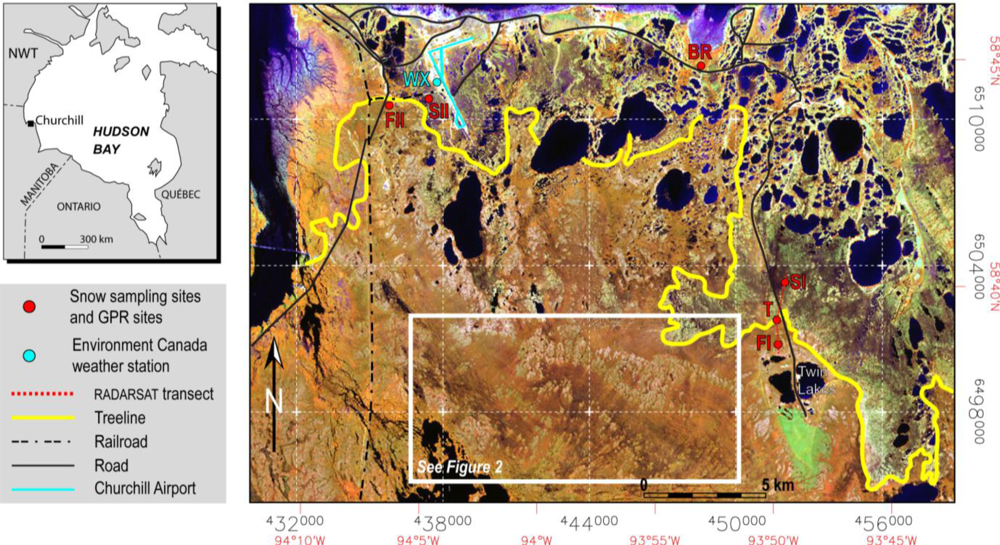
Churchill is located in northwestern Manitoba, Canada, at latitude 59°N; this area is dominated by wetlands, where the terrain elevation does not exceed 200 m (Figure 1). The region encompasses the southern limit of the continuous permafrost zone and the northern limit of the treeline and continuous forest [24]. Churchill falls within the High Subarctic ecoclimatic zone, which is characterized by a strong climatic gradient, where the boreal forest-tundra transition zone dominates. At the local scale, the influence of edaphic conditions (e.g., the micro-topoclimate, slope, soils, and drainage) combines with the influence of the dominant winds from Hudson Bay to create a complex vegetation mosaic [25]. The juxtaposition of various terrain types with different degrees of roughness and aerodynamic properties influences the snow accumulation patterns [23].
In August 1997, we surveyed vegetation at six sites, which were selected to represent the major terrain types found around Churchill. Figure 1 shows the location of the sites and their positions relative to a treeline that crosses the study area along a northwest-southeast-oriented diagonal. The Landsat ETM+ color composite image in Figure 1 was acquired on 18 August 2001. The area shown is approximately 560 km2 (28 × 20 km). The areas colored burnt orange below the treeline are open coniferous forest. Above the treeline, the dark-greenish-brown areas are wetlands, the bright orange areas are shrub formations, and the tea-green region is tundra. The large green patch on the glacial kame south of the Twin Lakes is a recovering burned area.
We conducted snow surveys at these sites during the two winters following our initial vegetation survey. These snow surveys revealed significant spatial heterogeneity in the snow cover conditions, which is similar to the observations reported in [19] and [20]. We noted a significant difference between open and closed areas and the transition zone in between. Additionally, the sites in the southeast, near the Twin Lakes differ from those in the northwest, near Churchill Airport (see Figure 1). Below, we describe the winter snow-cover characteristics and the vegetation and soil types at the sampling sites to illustrate how the snow accumulation is irregularly distributed across the Churchill landscape.
Site BR is located near the shore of Hudson Bay on a raised beach ridge with a poorly developed sandy soil that supports xerophytic plants, especially lichen and heath species, as per the description in [26]. The site itself corresponds to shrub tundra with lichens and sedges. Approximately half the surveyed surface is occupied by dwarf glandular shrubs. The snow cover remains shallow all winter long; the site is highly exposed without a protective vegetation cover, resulting in a significant removal of the snow by wind. The snow depth does not exceed 20 cm; the water equivalent increases slightly throughout the winter, along with the density, but remains below 50 mm. The cold, dry, and coherent snow on the surface is easily collected by the wind and then transported and captured by tall shrubs growing a short distance away.
Not far from the Twin Lakes, site SI is in a sedge fen characterized by a high water table and a hummock-hollow microtopography. The sedges (Carex aquatilis, Eleocharis palustris) cover 40% to 50% of the site surface. Additionally, less than 1% of this site is composed of small tamaracks (Larix laricina), and highly scattered shrubs (Betula glandulosa, Ledum decumbens, and Salix arctophila) cover less than 10% of the surface. The hummocks are 60 cm in height on average and are covered by xerophytic plants and a number of lichen and moss species similar to those ordinarily encountered in shrub tundra. However, the hollows are covered by mosses (especially Scorpidium turgescens) and a few sedges, which can either be wet or dry as the water table fluctuates. Forest site I (FI) is in an open coniferous forest, in which black (Picea mariana) and white (Picea glauca) spruces dominate. As in the sedge fen, the forest floor is an arrangement of hummocks and hollows, with moss and lichen communities covering much of the surface and standing water in the deeper hollows. Glandular birch (Betula), willow (Salix), and Labrador Tea (Ledum) shrubs are dispersed throughout the site. The topsoil is a fibrous peat layer approximately 30 cm thick that overlays clay-silt sediments.
The ground-measured snow depths are twice as high in this open coniferous forest (approximately 60 cm) than in the more open areas of the sedge fen (approximately 30 cm). However, the water equivalents are approximately the same. The differences in snow density can be readily explained by the disparities in snow depth between these two sites. For example, on 25 March 1998, the snow water equivalent and density were 84 mm and 259 kg·m−3, respectively, at SI; however, at FI, these values were 96 mm and 142 kg·m−3, respectively. Wind acts as the determining factor for snow density in treeless areas during accumulation (i.e., the fresh snow density is higher in areas exposed to wind), and over time, the snow matures (through snow packing and the formation of wind crusts). On 20 February 1998, we recorded snow water equivalents ranging from 20 to 115 mm along two 50-m transects at SI; however, the snow water equivalents at FI only varied from 60 to 90 mm. The presence of wind explains the heterogeneity of snow distribution at the fen site. Conversely, trees form a natural barrier to wind, and such a barrier considerably reduces the erosion and redistribution of snow by wind. Benefiting from the effective protection, the snow cover at FI tends to be less compact and more homogeneously distributed. We recorded no traces of wind crusts at the surface of the FI snowpack during either winter; however, meltwater crusts were found, which formed after midwinter short-term melt events.
At site SI, the snowpack consists of several dense and superimposed snow layers, each composed of rounded grains (ø= 0.5 mm); the underlying layers consist of coarser snow particles, mainly of the faceted-crystal type. The vertical sequence of low and hard snow layers at the top of the snow cover testifies to the occurrence of alternating accumulation and ablation events, with the latter resulting in the formation of wind crusts within the first few centimeters of the snow cover. The weak thermal gradient between the surface and the bottom of the snowpack at SI is not conducive to the formation of a thick layer of depth hoar. This shallow snow cover is a weakly porous medium, mainly composed of coherent, rounded-grain layers with a high thermal conductivity. As a result, the transmission of cold air through the snowpack is fast and efficient. At the end of the summer of 1997, the Churchill region received an unusually large amount of rain, which raised the water table above the surface and increased the depth of ponded water in the fen immediately prior to the fall freeze-up. As a result, the following winter’s snowpack at SI rested upon a thick layer of black ice, which prevented the geothermal heat flux from warming the bottom layers of the snow. The gravel road constructed directly through the fen acts as a barrier to the flow of water; therefore, this ice layer is likely to form when the water table is high, shortly before freeze-up.
The snow cover at FI has a relatively constant density of 150 kg·m−3 and therefore acts as an excellent insulator. This snow cover lies over a comparatively thick substrate of frozen moss and sphagnum, which is effectively warmer than the basal ice encountered at the fen site. The temperature registered at the snow-ground interface remains approximately 0 °C, and the thermal gradient through the snow cover exceeds 10 °C·cm−1. The heat surplus released through the geothermic flux sublimates the snow and produces a significant quantity of depth hoar (ø= 2–4 mm cups) in the layers closest to the ground. Additionally, the heat flux produces faceted crystals (ø= 1–2 mm) in the upper portion of the snowpack.
In the transition zone (T), the fen becomes increasingly covered by trees as one moves from SI to FI. The water table is very high during the summer in this area. The trees are predominantly represented by tamaracks. Much of the sampling area (50% to 60%) is densely covered by tall shrubs (mainly Betula glandulosa). The deepest snow cover can be found in this transition zone. The average snow depth and water equivalent are 80 cm and 155 mm, respectively. These parameters generally increase parallel to the vegetation gradient; they are lower in the vicinity of the fen (SI) and increase with increasing proximity to the open forest (FI). The transition zone is an efficient snow trap during snow-blowing events. Here, the trees are more widely spaced than in the open spruce forest; therefore, the wind-blown snow particles more easily penetrate into the transition zone. Then, the canopy of tall shrubs effectively catches the snow particles in suspension. The snow cover stratigraphy combines the characteristics of both the fen and the open forest snowpack, and the density is approximately intermediate. As in FI, the temperature at the snow-ground interface is approximately 0 °C, favoring the development of a thick basal depth hoar layer (approximately 30 cm in thickness).
Sites SII and FII, which are in the vicinity of the airport, are only 4 km from the coast; however, SI and FI are situated 14 km farther inland (see Figure 1). We know from [19] that falling snow near Churchill is largely eroded and blown southward off the exposed surfaces of Hudson Bay and the adjacent lowlands into the woodlands and eventually across the treeline and into the open forest. The accumulation rates at treeline can be as high as three times the measured rate of snowfall, depending on the wind speed and direction. The transport of blowing snow is usually estimated as a function of wind speed [27]. Because the wind speed typically decreases with movement inland, we can logically assume that SII and FII collect larger amounts of wind-blown snow than SI and FI, due to their relatively reduced proximity to the littoral zone. The wind transport interacts locally with vegetation at SII and FII to create a more irregular snow distribution pattern. SII is in the partially forested section of a fen. Moreover, the shrub cover is fairly dense compared with that of SI. At FII, the black and white spruces together with the tamaracks form a more continuously open canopy than at FI. Additionally, the basal peat layer is thicker at FII, and taller shrubs cover nearly 50% of the ground. Due to these differences in the vegetation architecture, we observed that the dispersion in snow water equivalent at these sites, which was measured based on the coefficient of variation, is as much as double that of the sites near the Twin Lakes. The wind action also translates into a finer stratification of the upper portion of the snowpack, which presents as multiple successions of thin, softer (accumulation strata) and harder (wind crusts) layers of snow, at both SII and FII. The difference in subsoil characteristics and shrub density causes both an increased variation in the vertical vapor exchanges and a reduction in the density and cohesiveness of the basal layers of snow at FII. During the study years, the bottom 20 cm of the mid-winter snowpack was composed of unusually dense (280 kg·m−3) and highly cohesive depth hoar with an average grain-size of 2–4 mm at FI and large grain-size (4–10 mm) depth hoar with low density (180 kg·m−3) and poor cohesiveness at FII. These observations are consistent with those made by [28], who found that in the arctic tundra, shrubs not only affect the distribution but also the structure and thermal characteristics of snow. More abundant and larger shrubs have a tendency to trap greater amounts of drifting snow and allow less loss due to sublimation, which leads to a deeper snow cover; these shrubs are also responsible for a greater proportion of the weakly bonded depth hoar of low thermal conductivity in the snowpack.
3. Data Collection and Processing
3.1. Ground-Based Snowpack Measurements
The snow-cover measurements were taken at 12.5-m intervals along two perpendicular transects 50 m in length. Shorter intervals were used where high winds had greatly redistributed the snow. To sufficiently characterize the snow cover, at least nine measurements were collected at each site, the locations of which are shown in Figure 1. In the transition zone, where the spatial variability of snow depth was greatest, we augmented the length of one of the two transects (100 × 50 m). Graduated snow stakes were inserted to a depth of 30–50 cm into the ground prior to the 1997/98 winter survey to mark the location of each sample to be collected. At every site, we proceeded with the following: (1) the collection of double readings of the snow depth at the stakes, carried out with a metal probe; (2) the extraction of snow cores using a model ESC-30 sampling tube to estimate the snow density and the snow water equivalent; and (3) the use of snow pits to profile the stratigraphy, grain size, temperature, and dielectric properties of the snow cover. The dielectric constant was measured using a flat-plate capacitive sensor operating at a frequency of 20 MHz [29]. The snow measurements were carried out to coincide with the RADARSAT-1 overpasses.
3.2. RADARSAT-1 and ERS-2 Imagery
RADARSAT-1 and ERS-2 C-band (5.3 GHz) synthetic aperture radar (SAR) images were acquired during the winters of 1997/98 and 1998/99. RADARSAT-1 sends and receives radar waves with horizontal polarization. This satellite offers a variety of beam modes and positions, with predefined incidence angle ranges, swath widths, and spatial resolutions. A total of 14 RADARSAT-1 standard beam mode images were used in the present study, provided by the Manitoba Remote Sensing Centre and the Canada Centre for Remote Sensing (Table 1). Twelve images were taken during the early morning descending orbit at 6:35 a.m., local time (±20 min). The images from 1 April and 19 May 1999, were acquired on the ascending orbit of RADARSAT-1 at 6:41 p.m., local time. Multi-incidence angle images, with angles ranging from 20°to 49°(S1 to S7 modes), were selected to meet the requirements of another study investigating the effect of incident angle variations on lake ice backscattering [18]. The repeat cycle of RADARSAT-1 is 24 days, but with different look angles, the system provides a 1- to 2-day repeat coverage at high latitudes. The finer temporal resolution of RADARSAT-1 makes it more attractive than ERS-2 for monitoring processes that evolve rapidly, such as the spring snowmelt.
The ERS-2 satellite C-band SAR operates with VV polarization and does not have the multi-incidence angle capability of RADARSAT-1. The fixed-look angle of ERS-2 ranges from 20.1° to 25.9°across a given image, which can be roughly compared to the S1 mode of RADARSAT-1. The ERS-2 images were acquired on the descending orbit at approximately 6:20 a.m., local time, for the following eight dates: 18 February 1998, 9 March 1998, 13 April 1998, 18 May 1998, 5 October 1998, 9 November 1998, 14 December 1998 and 29 March 1999.
Both sets of SAR images have a nominal resolution of approximately 25 m and a pixel spacing of 12.5 m. All images were radiometrically calibrated at the Canadian Data Processing Facility using the most recent antenna pattern correction and payload parameter file. Using the PCI Geomatics/Geomatica image processing software [30], the processor-applied look-up table was removed from all images to generate calibrated radar backscatter images. As reported in [22], a local slope angle of 0° was used, which is a realistic assumption given the very flat topography of the study area. The geometric distortions were corrected using both image ephemeris data and ancillary ground control points (GCPs). Between 15 and 20 GCPs were selected from topographic maps, and the first RADARSAT-1 image (image to map registration) was georectified by applying a third-order polynomial and a cubic convolution resampling algorithm. This reference image was used afterward to correct the other scenes (image-to-image registration). An accuracy on the order of 1 pixel, in terms of the root-mean-square error, was achieved. By comparing the pixel displacement across the images for easily identifiable and known landmarks, such as the railroad and roads, the airport runway, seaport buildings, the Churchill Rocket Research Range, and the shipwreck of the M/V Ithaca in Bird Cove, we estimated the accuracy of the georeferencing to be 1–3 pixels (i.e., 12.5–37.5 m). For each image, 5 × 5 windows (25 pixels) centered on the snow sampling sites were extracted, and standard statistics were computed from the backscatter power values and then converted to backscattering coefficients (σ0) in decibels (dB).
3.3. Ground-Penetrating Radar Surveys
A PulseEkko 1000 ground-penetrating radar (GPR) instrument was also used to image the subsurface and the interior of the snow pack. GPR operates with a set of antennas: the first transmits successive radar impulses that are reflected by the dielectric discontinuities between the snow pack and the subsurface, and the second receives the signal that is reflected back toward the (snow) surface. The antennas are positioned in a fiberglass box and connected with coaxial cables to a control unit that digitizes the electric signals recorded by the receiving antenna. The control unit amplifies, processes, and then stores the information received by the antenna; examples of such information are the travel time between the transmitted and reflected signal and the amplitude and frequency of the reflected radar waves. A more thorough description of GPR can be found in [31]. In the vicinity of the six snow sampling sites, we conducted two types of GPR surveys: reflection profiling and common mid-point (CMP) velocity sounding. In the reflection profiling mode, the transmitting and receiving antennas were attached relative to each other with a constant separation of 15 cm and were then moved manually along a transect 9 m in length. We then obtained a profile showing the temporal location of the radar echoes as a function of the distance surveyed on the ground. The CMP velocity sounding is the electromagnetic equivalent of the seismic profile. The transmitting and receiving antennas were moved away from each other in 1-cm increments while maintaining a common mid-point. The GPR data collected in CMP mode were used to estimate the signal velocity in the snow pack and the subsurface to convert the time scale of the GPR reflection profiles into a depth scale. The stratigraphic information from traditional snow profiles was used to identify and determine the depth of both the snow–ground interface and the various reflectors within the snow pack with a precision of approximately 2 cm. A detailed description of this experiment is reported in [32].
4. Results and Discussion
The qualitative interpretation of C-band radar backscatter measurements gathered over the heterogeneous environment under study requires an understanding of the scattering mechanisms involved. The basic backscattering behavior of snow-covered terrain is described by scattering models that have been supported by experimental results, such as [33] and [34]. According to these models, the total backscattered signal from the snow-covered terrain consists of surface and volume contributions, including surface scattering at the air–snow interface, volume scattering by the snow layer, and surface scattering at the snow–ground interface, which is attenuated by the snow layer. For dry snow conditions, C-band radar waves can penetrate easily (i.e., approximately 10 m at a snow density of 200 kg·m−3 [35]), and the dielectric contrast at the air–snow interface is low. As a result, the scattering at the snow surface is independent of the snow surface roughness and can be ignored. The total backscatter signal of dry, snow-covered terrain is therefore a combination of the snow volume scattering and the surface scattering from the ground. The C-band backscatter is largely dominated by (rough) surface scattering from the ground–snow boundary for typical dry snow conditions. Volume scattering can become more important when large snow grains (i.e., depth hoar) or thicker snow packs (>1 m) are present [36]. The presence of liquid water within the snow pack results in high dielectric contrast at the air–snow boundary and a high absorption loss, which greatly reduces the penetration. For wet snow conditions, the total backscattering is governed by rough-surface scattering at the air–snow boundary and absorption losses within the snow layer; thus, scattering from the snow–ground interface can be ignored.
The scattering models in [33,34,36] are focused on soil and snow properties and ignore the effect of vegetation and trees. Theoretical and semi-empirical scattering models for the C-band backscatter of the forest–snow–ground system in dense to open boreal forests are presented and discussed in [16,37,38]. These models further differentiate among the respective contributions of the forest canopy, snow cover, and ground surface.
4.1. Spatial Variations in the RADARSAT-1 Backscatter at the Time of Peak Snow Accumulation
To examine the effect of dry snow on the backscatter of C-band radar, we first visually compared two RADARSAT-1 images acquired with the same incident angle (20–27°, S1 mode) at the time of peak snow accumulation in different snow seasons (Figure 2). The radar backscatter values were linearly stretched using identical minimum and maximum values. Overall, the radar backscatter from snow-covered ground is higher (i.e., higher brightness) in the 1998 image than in the 1999 image. The 1998 image also shows a greater spatial variability (i.e., small- to large-scale variations in contrast), as highlighted by the white box in Figure 2.
We hypothesize that the differences in backscatter are representative of variations in the snow conditions, with the backscatter increasing as the snow water equivalent increases (i.e., a positive relationship); this would imply that more snow had accumulated by the end of winter 1997/98 than by the end of winter 1998/99. Furthermore, we can infer from the spatial heterogeneity of the backscatter that the larger volume of snow was subject to greater redistribution by the wind.
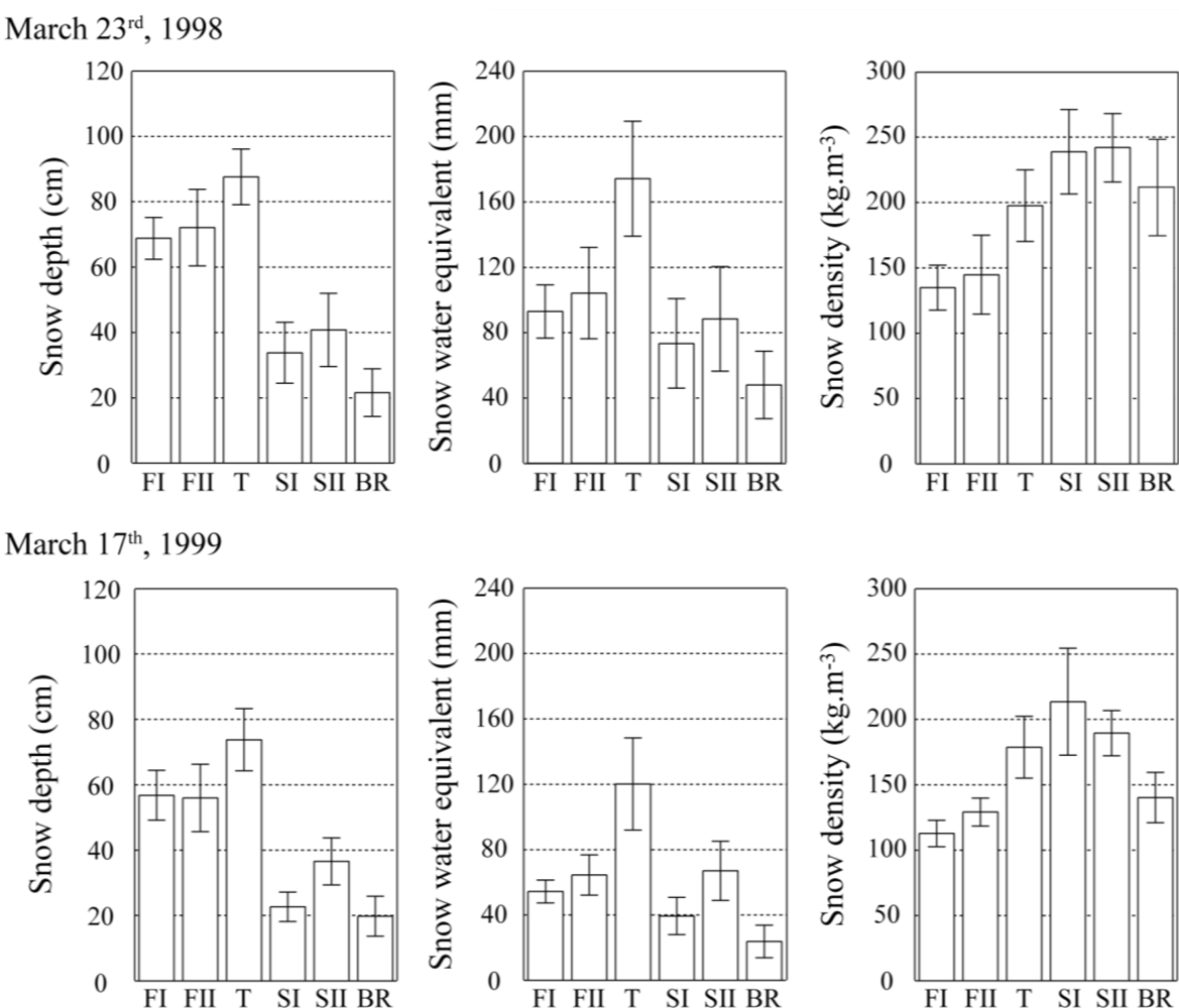
The in situ snow measurements (Figure 3) made at the time of the RADARSAT-1 overpasses are actually consistent with this assumption. The snow cover was of greater depth in March 1998 than in March 1999, except at the tundra site near the shore (BR). Specifically, the snow cover exceeded 60 cm in the open forest, 80 cm in the transition zone, and 35 cm in the fen, i.e., the snow cover was approximately 10–15 cm thicker in March 1998 than in March 1999.
The snow water equivalent measurements reveal the actual amount of snow that accumulated. Between the two winters, we observed a difference of 20–25 mm water equivalent at BR, SI, SII, and FI and as much as 40–50 mm at FII and T. At BR, where the snow depth remained unchanged, there was actually twice as much snow in March 1998 as in March 1999. The greater amount of snow on the ground in 1998 introduced additional snow compaction, which translated into the higher snow density values. This is particularly true for the BR observation site, where the snow density was 210 kg·m−3 (1998) versus 140 kg·m−3 (1999).
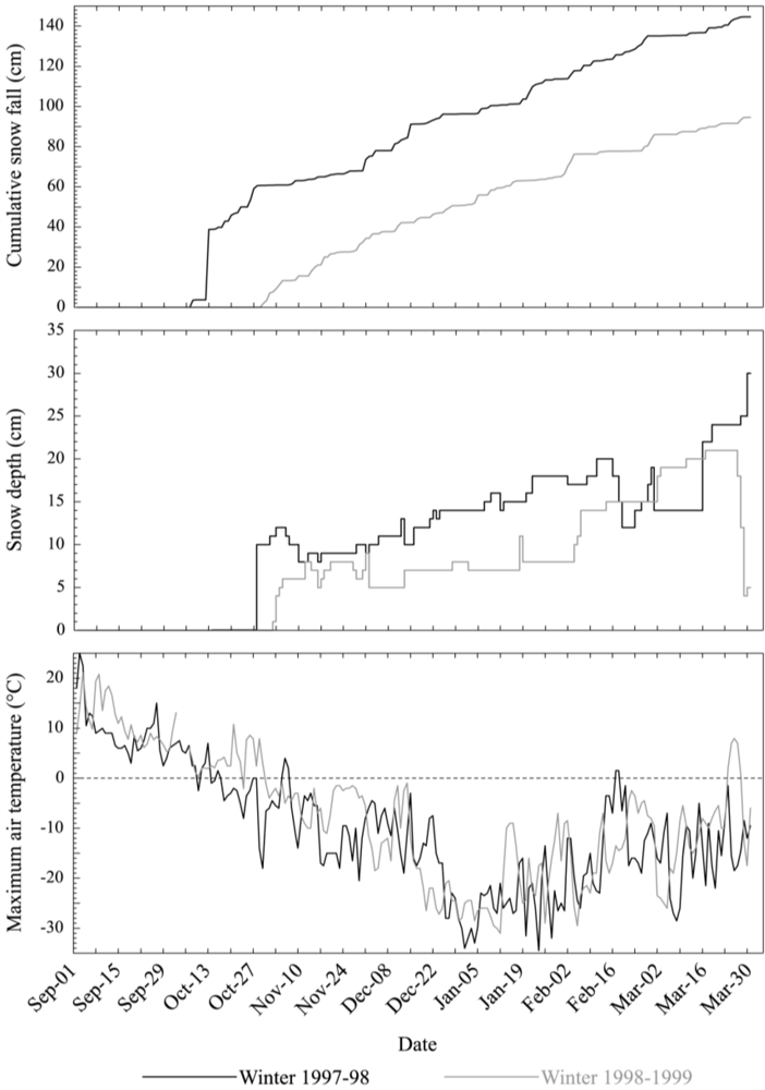
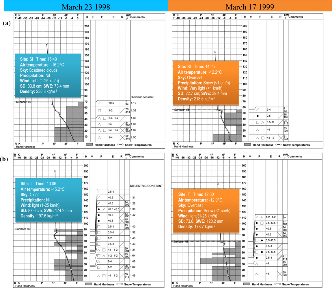
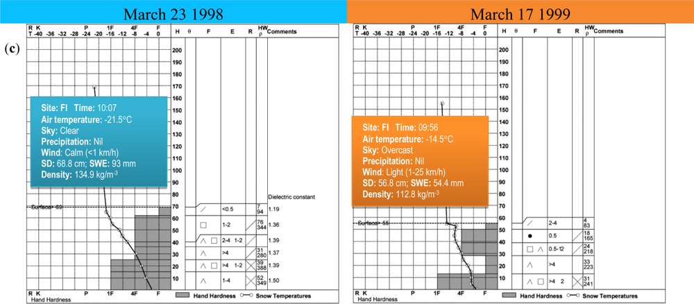
The snowfall and depth records at the Churchill Airport weather station indicate that snow accumulation commenced later in the winter of 1998/99 than in the winter of 1997/98 (Figure 4). The cumulative snowfall trend indicates that the first ground-accumulating snow was delayed by approximately 1.5 months. Considerably less snowfall (approximately 50 cm less) was recorded at the airport in 1998/99, which is consistent with the lower snow accumulation that we observed at the sampling sites. The late accumulation of snow in 1998/99 translated into a more homogeneous snow cover, as suggested by the smaller standard deviation of the snow water equivalent at every site (Figure 3) and by the snowpack stratigraphy. There were fewer discernible snow layers in March 1999 than in March 1998 in the sedge fen (Figure 5(a)) and in the transition zone (Figure 5(b)) snow cover. Furthermore, the thicker snowpacks of the open forest (Figure 5(c)) and the transition zone underwent greater metamorphic transformation in March 1998. The higher proportion of faceted crystals and depth hoar indicates a more advanced stage of constructive metamorphism of the snowpack. In contrast, the presence of more fine, rounded grains in March 1999, even in the lower horizons, indicates more recent accumulations.
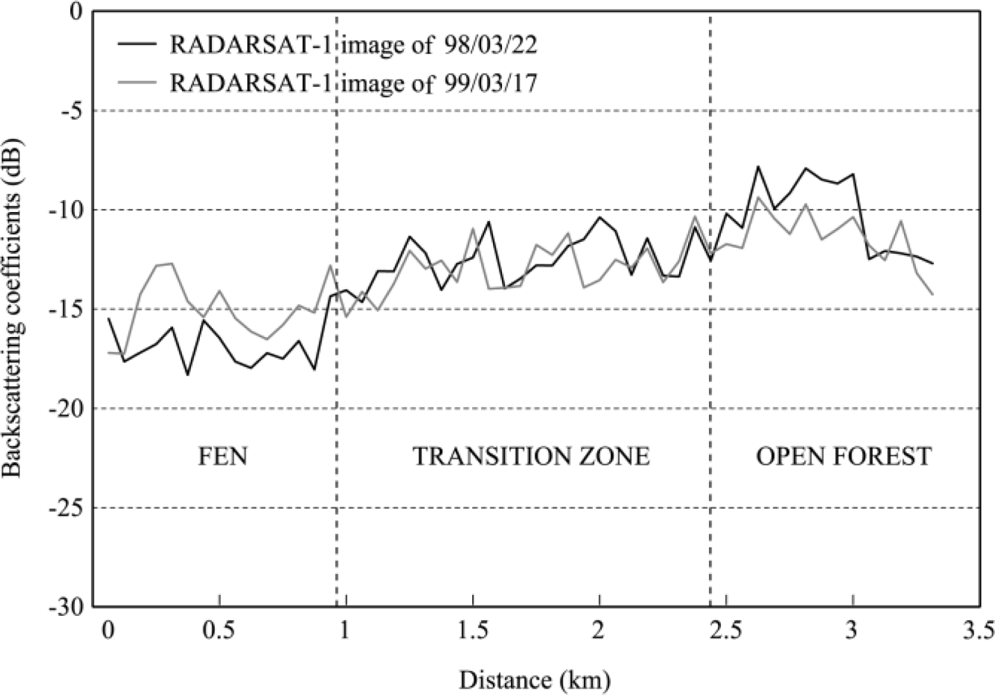
Regrettably, the information that we obtained from the fluctuations of the average backscattering coefficients along a 5-pixel-wide (62.5 m) and 3.5-km-long transect passing near FI, T and SI (see Figure 1) seems to involve a much more complex set of spatial patterns influencing the end-of-winter radar backscatter in the Churchill area (Figure 6). In March 1998, the backscatter values gradually increased from the open to the forested areas, with a significant difference between them. The backscattering coefficients fluctuated between −20 and −15 dB in the sedge fen and between −15 and −9 dB in the transition zone, and they exceeded −10 dB in the open coniferous forest. Closer to Twin Lake West, the radar signal significantly decreased.
This transect shows an increase of the backscattering coefficient from the open areas to the forested areas; this increase is mostly due to the vegetation gradient. The presence of short vegetation (h < 30 cm) is usually insufficient to affect the backscattering from snow-covered surfaces, such that the soil liquid water content and the surface roughness contribute most of the signal, to a degree that varies as a function of the angle of incidence [39]. The forest is a strong scatterer of radar energy to varying degrees, depending on the density, structure and composition of the forest [40]. For example, C-band radar signals are effectively scattered by coniferous needles, especially at the HH polarization, whereas the contribution of branches dominates at the VV polarization [34]. Scattering by trees is one of several factors affecting the radar signal, either from the ground or the snow cover. The stem volume is known to mask the effects of snow to some degree [41]. This effect was quantified by [42] for the Finnish boreal forest. These authors found that 93% of the variance of the C-band backscatter of snow-covered forests in the VV polarization could be explained by the stem volume. Additionally, the stem volume, snow wetness, and snow water equivalent together were sufficient to explain 80% of the variance of the C-band HH-polarized backscatter. In the present study, the vegetation physiognomy did not change within a year along the 3.5-km transect. However, the difference in backscatter between the open and forested areas was much less significant in March 1999; the difference was approximately 7 dB in March 1998 but only 3 dB in March 1999. However, only the open forest exhibited the expected decrease in radar intensity with a reduced snow water equivalent. Elsewhere, either the backscatter values did not change (e.g., in the transition zone) or they increased by approximately 2 dB (e.g., in the open areas).
4.2. Seasonal Variations of the RADARSAT-1 and ERS-2 Backscatter
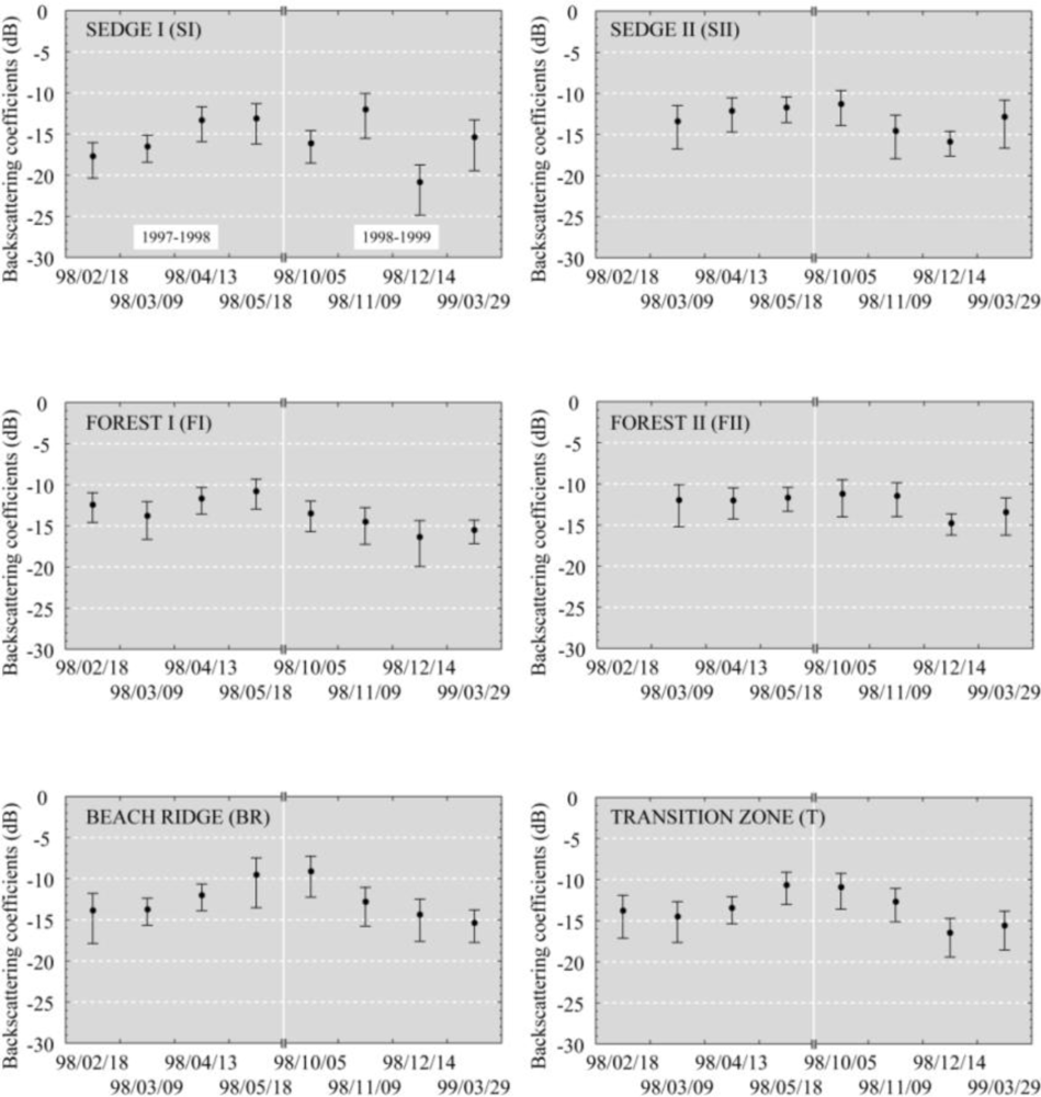
Next, we consider the ability of RADARSAT-1 (Figure 7) and ERS-2 to express the seasonal changes in surface conditions (ground, vegetation, and snow). We are limited, however, by the fact that the available images were acquired under (very) different viewing conditions, with incidence angles varying from 20°to 49°.
4.2.1. The Effect of the Incidence Angle
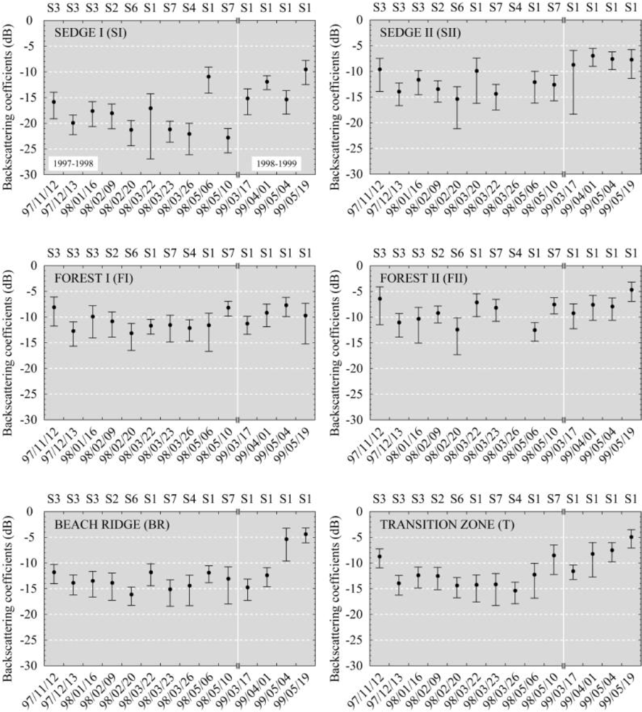
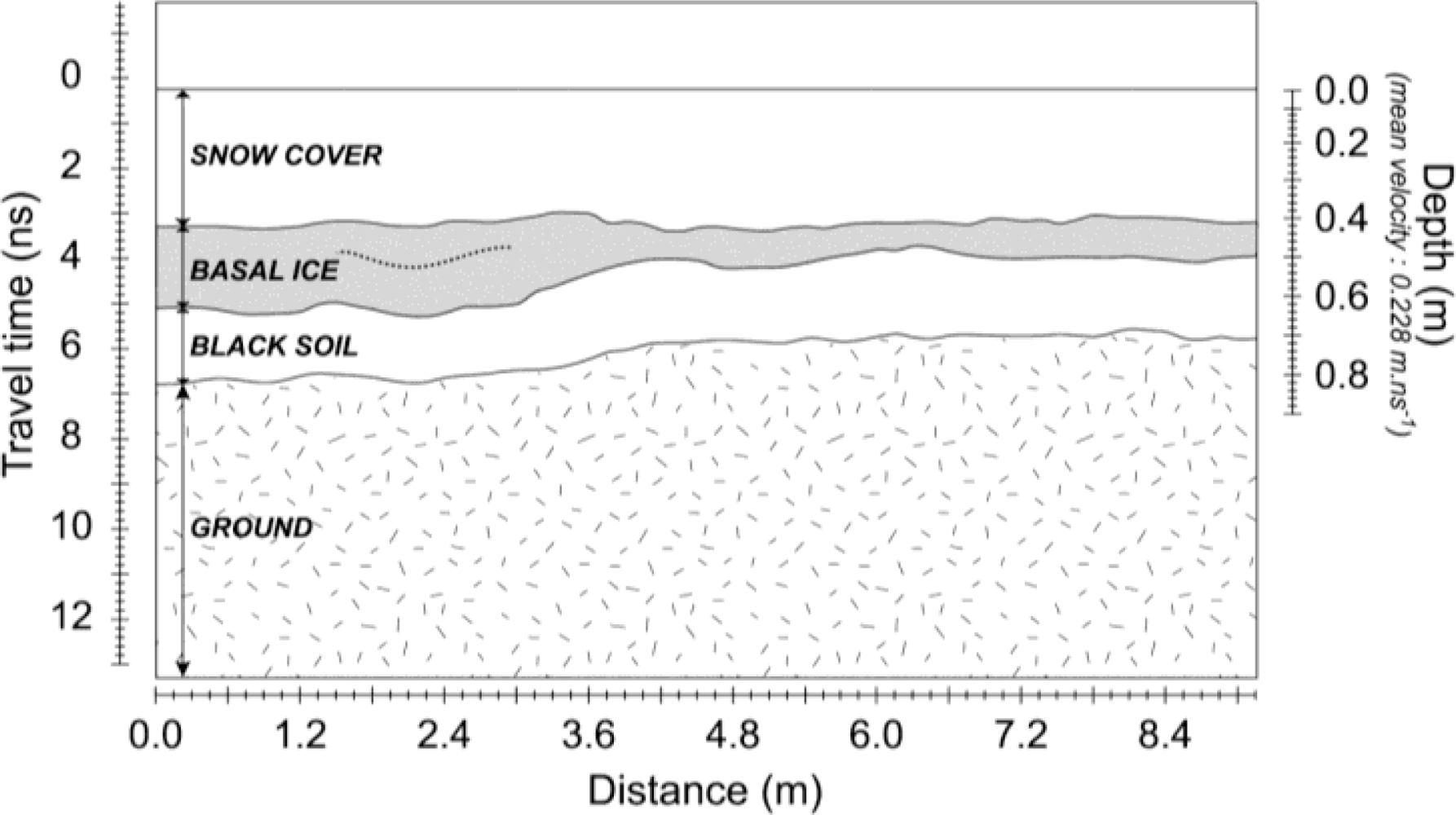
In Figure 7, the effect of incidence angle on the RADARSAT-1 backscatter is evident. With unchanged snow conditions at the sedge fen site (SI), the backscattering coefficients dropped abruptly, by more than 4 dB, between the 22nd (S1 mode; 20–27°incidence angles) and the 23rd (S7 mode; 45–49° incidence angles) of March 1998. The uneven topography and a 10–20-cm layer of black ice underneath the snow cover were detected in the field by the use of high-frequency (900 MHz) GPR at site SI (Figure 8).
The thickness of this layer, as estimated through the ground-penetrating radar survey, agrees with the direct (stake) measurements gathered in the field. The thickness of the under-snow ice was estimated by comparing the manually probed snow depths with the observations of snow in relation to the stakes at the measuring stations, where the zero marks were positioned at the ground surface before the occurrence of the unusually wet conditions in late summer, as previously described. This subsurface feature likely contributes to a modification of the winter radar signature at this site (i.e., a low radar return), especially at higher incidence angles. Due to the low dielectric contrast at the ice–ground interface, much of the signal passes into the frozen soil, where it is absorbed, reducing the signal returned to the radar detector [43,44]. At greater incidence angles, specular reflection occurs at the ice–ground interface, which is smooth in relation to the C-band frequency, and dominates the radar signal.
In spring 1998, the sedge fen (SI) turned into a vast pool of standing meltwater. The strong specular reflection off the smooth water surface occurring at larger incidence angles caused an even more significant change in the backscatter intensity at SI (a difference of −11 dB), as recorded between the two images acquired in the S1 (6 May) and S7 (10 May) standard modes.
In contrast, the backscatter at the open coniferous forest site (FI) and transition site (T) did not change significantly between 22 and 23 March, and therefore seems to be more independent of the incidence angle. The C-band backscatter at this site is less sensitive to variations of the surface, and volume scattering in the forest canopy may be the dominant mechanism [42,45]. At FII, where the trees are spaced farther apart, more radar waves are able to penetrate to the ground, which results in enhanced surface scattering and a slightly larger dependence of the radar return on variations in the incidence angles.
4.2.2. The effect of soil freezing on backscatter in autumn and early winter
Three RADARSAT-1 images are available within the 30–37°incidence angle range (S3 mode) between November 1997 and January 1998 (Figure 7). Using these images, we can observe the evolution of the fall and early winter backscattering coefficients in 1997/98. Between 12 November and 13 December, the backscatter decreased at every site: by a factor of 2 dB in the coastal tundra, by 4.5 dB in the fen and open forest, and by more than 5 dB in the transition zone. The first snow was recorded on 14 October at the airport weather station. The region received at least 65 cm of cumulative snowfall by 12 November and an additional 20 cm by 13 December, which formed a shallow (8–13 cm), compact snow cover at the airport (Figure 4). The radar intensity was decreased considerably due to a simultaneous decrease of the permittivity of the soil and vegetation with freezing [26,37,46–48].
The ERS-2 backscatter values also decreased from 5 October (no snow) to 9 November (little snow) and 14 December (more snow) of the following winter by approximately 5 dB at most sites and slightly less at FI (Figure 9).
Although the snowpack was very shallow (<10 cm), the region received 80 cm of cumulative snow fall by 14 December. Once more, SI distinguished itself from the other sites, exhibiting a stronger radar return before dropping dramatically to −22 dB (i.e., a 10-dB difference). We believe that the surface water in the sedge fen was not completely frozen on 9 November. Radar backscatter can increase with freezing in areas of standing water, including wetlands, due to the formation of a rough ice–water or ice–soil interface [49]. During freezing conditions, the rate of decrease in the ERS-2 backscatter was more rapid at BR and SII and more gradual at FI, FII, and T, suggesting that areas with poor insulation from shallow snow cover are differentially frozen versus areas with greater snow accumulation and higher surface soil temperature.
The daily records of ground temperature at various depths near FII are given in Table 2. These records confirm that the decrease in radar backscatter in the fall coincided with the gradual penetration of the cold wave through the soil.
Before the soil freezes, the accumulation of snow on the ground surface does not significantly affect the backscatter values [39]. The ground temperature patterns in Churchill indicate that the soil must be frozen to depths greater than 20 cm before a snow effect can be observed on the C-band SAR signal. In the RADARSAT-1 image of January 16, where the ground was frozen to a depth of 50 cm, the backscattering coefficients increased by 1.5–2.8 dB at SI, SII, FI, and T compared with 13 December. No significant change was observed at BR and FII (less than 1 dB).
4.2.3. The Effect of the Dry Snow on Backscatter in the Mid-Winter to End of Winter
The RADARSAT-1 data are available within the 20–31° incidence angle range (i.e., S1 and S2 modes), allowing for the observation of changes from mid-winter to end-of-winter snow conditions (Figure 7). The lack of data makes it impossible to use a regression model to retrieve the snow water equivalent from the backscatter. However, systematic conclusions can be drawn from the data themselves. Between 9 February and 22 March 1998, the backscatter values increased by 2 to 3.5 dB in parallel with an increasing snow water equivalent, except for FI and T, where the backscatter values decreased by −0.8 and −1.7 dB, respectively. At SI, the backscatter only increased by 1 dB, which is less than the RADARSAT-1 relative radiometric accuracy of 1.5–2 dB for the standard beam modes [50]. Both images were acquired under dry snow conditions. Between the two dates, 11.5 to 19 mm of water equivalent were added to the snowpack at BR, SI, and FII, which corresponds to an average increase of 27%. At SII, where the largest positive change in radar intensity was observed, the snow water equivalent changed from 50 to 88 mm (a 74% increase). The slightly steeper incidence angle for the image from 22 March might explain some of the backscatter behavior observed at these sites, in addition to the increase in snow water equivalent. A negative dependence between the backscattering signal and incidence angle for the dry-snow-covered surfaces was indeed found in both the forested and non-forested areas [51,52]. At the sites where backscatter decreased, the change in snow water equivalent was variable: +17.5 mm at FI and +38 mm at T (a respective gain of 23% and 28%, respectively).
The correlation between the snow water equivalent and the radar backscatter depends on both the snow (snow density, stratigraphy, granulometry, and water content) and the ground (surface roughness and dielectric properties) parameters. Whenever the volume scattering from the snowpack is greater than the ground scattering attenuated by the snow, a positive correlation is expected. Otherwise, the correlation is negative [53]. For open areas (agricultural land) in Finland, such a positive linear trend between airborne backscattering coefficient data acquired by EMISAR at the C-band and ground measurements of the snow water equivalent was observed [38]. The correlation was slightly higher for the VV-polarized data (r = 0.79) compared with the HH-polarized data (r = 0.69), and the effect of dry snow on backscatter was more visible when the snow water equivalent values were greater than 50 mm, likely because of the decreased contribution from the ground. Specifically, the authors of [39] were unable to detect volume scattering within a shallow dry snow cover at the C-band because the radar return was dominated by the soil surface scattering. A semi-empirical model that accounts for this ground effect and that connects the thermal resistance of the snow with the backscatter signal was developed and tested in various environments to retrieve the snow water equivalent from the C-band SAR data [39,54,55]. The uncertainty analysis for this model can be found in [56].
The presence of a thick layer of ice underneath the snowpack at SI, whose presence was previously demonstrated (Figure 8), may explain the absence of a trend in fluctuating backscatter values with respect to changes in the snow water equivalent. Moreover, we observed that the dispersion around the average backscatter at SI was much greater than usual on March 22; consequently, 24% of the sampled pixels show backscatter values lower than −25 dB. It is difficult to determine, retrospectively, whether these are actual ground effects or simply noise signals or image artifacts.
The high-frequency GPR surveys at FII detected a 20–30-cm layer of peat underneath the snow, the presence of which was confirmed by the elementary soil sampling we performed in the summer of 1997 (Figure 10). The same thick organic layer was found at SII (whereas it was less than 5 cm at FI and T) and rapidly transitioned into mineral soil. The interactions within the snowpack–organic/mineral soils–backscatter system may also explain the difference in the trends observed at the different sites and should be investigated further.
4.2.4. Changes in Backscatter during the Post-Melt Period
No RADARSAT-1 image was recorded during the snowmelt, such that we were unable to verify the effect of wet snow on radar backscatter. During the first week of May 1998, most of the snow disappeared in the field, and only traces were recorded at the Churchill airport for that period. In the spring of 1999, the snowmelt occurred earlier and more rapidly (by one week) than usual. By 1 April, almost all the snow was gone; subsequently, the air temperature again fell below zero for approximately one week. The presence of frozen meltwater ponds and remnant refrozen snow caused higher backscatter in the S1 image of 1 April compared with that of 17 March (Figure 7). Finally, the images of May 1998 and 1999 are snow-free. The level of backscatter is much higher for snow-free ground than snow-covered. BR, T, SI, and FII (in decreasing order) show the largest differences (4.5–10 dB), whereas SII and FI differ by only 1–1.5 dB for 17 March.
5. Conclusions
During the winters of 1997/98 and 1998/99, we explored the ability of C-band SAR measurements to retrieve snow information, especially the snow water equivalent under dry snow conditions, in a forest-tundra environment. Multi-temporal RADARSAT-1 images over Churchill, northern Manitoba, were used as the main data source, in addition to some ERS-2 imagery, to study the C-band backscatter characteristics under snow conditions. Supporting field data were acquired, concurrent with the RADARSAT-1 overpasses.
The manual snow surveys demonstrated that the accumulation of snow across such a landscape is extremely irregular, due to the strong redistribution by wind and the spatial heterogeneity of the land cover. The comparison of field measurements and backscatter values enabled the identification of some impacts of the ground, vegetation, and viewing conditions, in addition to the snow-cover characteristics, on the seasonal variability of C-band radar backscatter at the treeline.
The contribution of dry snow to the C-band backscatter appears to be effective only when frost has penetrated the first 20 cm of the soil. Both RADARSAT-1 and ERS-2 measurements support this observation. Once this frost depth has been reached, the RADARSAT-1 backscatter began to respond positively to changes in the snow water equivalent, at least in the tundra (BR), sedge fen (SII), and open forest (FII) of the nearshore areas. For these sites, at small incidence angles (20–31°), 1-dB increases in backscatter occurred for every approximately 5–10 mm of water equivalent of accumulated snow depth. However, in the inland open and forested areas near the Twin Lakes and the transition zone between them, the backscatter increased only very slightly (e.g., SI) or even decreased with increasing snow water equivalent (e.g., FI and T). When backscatter is plotted against the transect vegetation, it gradually increases from the open areas (−17 to −15 dB) to the transition zone (−14 to −13 dB) to the forested areas (−12 to −10 dB). In sparsely vegetated areas, the RADARSAT-1 backscatter response from the dry snow cover was also found to be lower at larger incidence angles (45–49°) than at lower incidence angles (20–27°) by approximately 4 dB, whereas it remained unchanged in the forested and partially wooded areas. Combined, these observations support the hypothesis that the radar signal at these sites is dominated by ground surface scattering when not attenuated by the vegetation. For example, a 10–20-cm layer of black ice underneath the snow cover, as evidenced by a high-frequency GPR measurement, caused the very low radar return (i.e., 15 dB and less) observed at and around SI.
The observations of such diametrically opposed radar responses to snow water equivalent within the same study area are of interest, and the conditions that produced these distinct responses should be investigated further. For now, these results have informed us that a simple relationship between the snow water equivalent of the dry snow cover and the radar backscatter at C-band frequencies is unlikely to be found in environments as complex as forest-tundra without prior corrections for both vegetation and ground effects.
Acknowledgments
Financial assistance for the fieldwork was provided by the Climate Research Branch, Environment Canada, in support of the CRYSYS program and the Natural Sciences and Engineering Research Council of Canada. The work of F. Pivot was supported by the Ministère de l’Enseignement supérieur et de la Recherche in France through a doctoral grant. During that time, F. Pivot was with the Universitédes Sciences et Technologies de Lille, France. F. Pivot wishes to thank Roy Dixon of the Manitoba Remote Sensing Centre and Terry Pultz of the Canada Centre for Remote Sensing (CCRS) for providing the RADARSAT-1 and ERS-2 images, Tom Lukowski (CCRS) for helping with the calibration of the ERS-2 images, Anouk Utzschneider for her assistance with the geometric correction of the ERS-2 images, and Denis Sarrazin (Centre d’Études Nordiques, Université Laval) for his technical assistance in the field. She is also grateful to the Churchill Northern Studies Centre for the logistical support provided during the field campaigns. Finally, F. Pivot would like to express her gratitude to her doctoral supervisors: Claude Kergomard, now at the Department of Geography of the École Nationale Supérieure (France), and Claude Duguay, director of the Interdisciplinary Centre on Climate Change at the University of Waterloo (Ontario, ON, Canada).
References
- Scherer, D.; Hall, D.K.; Hochschild, V.; König, M.; Winther, J.-G.; Duguay, C.R.; Pivot, F.; Mätzler, C.; Rau, F.; Seidel, K.; et al. Remote Sensing of Snow Cover. In Remote Sensing in Northern Hydrology: Measuring Environmental Change; Duguay, C.R., Pietroniro, A., Eds.; Geophysical Monograph 163; American Geophysical Union: Washington, DC, USA, 2005; pp. 7–38. [Google Scholar]
- Nagler, T.; Rott, H. Retrieval of wet snow by means of multitemporal SAR data. IEEE Trans. Geosci. Remote Sens 2000, 38, 754–765. [Google Scholar]
- Longepe, N.; Allain, S.; Ferro-Famil, L.; Pottier, E.; Durand, Y. Snowpack characterization in mountainous regions using C-Band SAR data and a meteorological model. IEEE Trans. Geosci. Remote Sens 2009, 47, 406–418. [Google Scholar]
- Huang, L.; Li, Z.; Tian, B.; Chen, Q.; Liu, J.; Zhang, R. Classification and snow line detection for glacial areas using the polarimetric SAR image. Remote Sens. Environ 2011, 115, 1721–1732. [Google Scholar]
- Liu, H.; Wang, L.; Jezek, K.C. Automated delineation of dry and melt snow zones in Antarctica using active and passive microwave observations from space. IEEE Trans. Geosci. Remote Sens 2006, 44, 2152–2163. [Google Scholar]
- Brown, I.A.; Sandgren, E. Investigation of the spatial variations in synthetic aperture radar backscatter in Western Dronning Maud Land, Antarctica. J. Appl. Remote Sens 2008, 2, 023509. [Google Scholar]
- Geldsetzer, T.; Yackel, J.J. Sea ice type and open water discrimination using dual co-polarized C-band SAR. Can. J. Remote Sens 2009, 35, 73–84. [Google Scholar]
- Eriksson, L.E.B.; Borenas, K.; Dierking, W.; Berg, A.; Santoro, M.; Pemberton, P.; Lindh, H.; Karlson, B. Evaluation of new spaceborne SAR sensors for sea-ice monitoring in the Baltic Sea. Can. J. Remote Sens 2010, 36, 56–73. [Google Scholar]
- Baghdadi, N.; Gauthier, Y.; Bernier, M. Capability of multitemporal ERS-1 SAR data for wet-snow mapping. Remote Sens. Environ 1997, 60, 174–186. [Google Scholar]
- Baghdadi, N.; Fortin, J.-P.; Bernier, M. Accuracy of wet snow mapping using simulated Radarsat backscattering coefficients from observed snow cover characteristics. Int. J. Remote Sens 1999, 20, 2049–2068. [Google Scholar]
- Koskinen, J.T.; Pulliainen, J.T.; Hallikainen, M.T. The use of ERS-1 SAR data in snow melt monitoring. IEEE Trans. Geosci. Remote Sens 1997, 35, 601–610. [Google Scholar]
- Pulliainen, J.T; Kurvonen, L.; Hallikainen, M.T. Multitemporal behavior of L- and C-band SAR observations of boreal forests. IEEE Trans. Geosci. Remote Sens 1999, 37, 927–937. [Google Scholar]
- Kurvonen, L.; Hallikainen, M.T. Textural information of multitemporal ERS-1 and JERS-1 SAR images with applications to land and forest type classification in boreal zone. IEEE Trans. Geosci. Remote Sens 1999, 37, 680–689. [Google Scholar]
- Luojus, K.P.; Pulliainen, J.T.; Blasco Cutrona, A.; Metsamaki, S.J.; Hallikainen, M.T. Comparison of SAR-based snow-covered area estimation methods for the boreal forest zone. IEEE Geosci. Remote Sens. Lett 2009, 6, 403–407. [Google Scholar]
- Santoro, M.; Fransson, J.E.S.; Eriksson, L.E.B.; Magnusson, M.; Ulander, L.M.H.; Olsson, H. Signatures of ALOS PALSAR L-band backscatter in Swedish forest. IEEE Trans. Geosci. Remote Sens 2009, 47, 4001–4019. [Google Scholar]
- Koskinen, J.T.; Pulliainen, J.T.; Luojus, K.P.; Takala, M. Monitoring of snow-cover properties during the spring melting period in forested areas. IEEE Trans. Geosci. Remote Sens 2010, 48, 50–58. [Google Scholar]
- Dean, A.M.; Brown, I.A.; Huntley, B.; Thomas, C.J. Monitoring snowmelt across the Arctic forest-tundra ecotone using Synthetic Aperture Radar. Int. J. Remote Sens 2006, 27, 4347–4370. [Google Scholar]
- Bergengren, J.C.; Waliser, D.E.; Yung, Y.L. Ecological sensitivity: A biospheric view of climate change. Climatic Change 2011, 107, 433–457. [Google Scholar]
- Scott, P.A.; Hansell, R.I.; Erickson, W.R. Influences of wind and snow on northern tree-line environments at Churchill, Manitoba, Canada. Arctic 1993, 46, 316–323. [Google Scholar]
- Kershaw, P.G.; McCulloch, J. Midwinter snowpack variation across the Arctic treeline, Churchill, Manitoba, Canada. Arct. Antarct. Alp. Res 2007, 39, 9–15. [Google Scholar]
- Gamache, I.; Payette, S. Height growth response of tree line black spruce to recent climate warming across the forest-tundra of eastern Canada. J. Ecol 2004, 92, 835–845. [Google Scholar]
- Duguay, C.R.; Pultz, T.J.; Lafleur, P.M.; Drai, D. RADARSAT backscatter characteristics of ice growing on shallow sub-arctic lakes, Churchill, Manitoba, Canada. Hydrol. Process 2002, 16, 1631–1644. [Google Scholar]
- Pivot, F.; Kergomard, C.; Duguay, C.R. On the use of passive microwave data to monitor spatial and temporal variations of snowcover near Churchill, Manitoba. Ann. Glaciol 2002, 34, 58–64. [Google Scholar]
- Rouse, W.R. Impacts of Hudson Bay on the terrestrial climate of the Hudson Bay Lowlands. Arctic Alp. Res 1991, 23, 24–30. [Google Scholar]
- Scott, G.A.J. Manitoba’s Ecoclimatic Regions. In The Geography of Manitoba, Its Land and Its People, 1st ed.; Welsteed, J., Everitt, J., Stadel, C., Eds.; The University of Manitoba Press: Winnipeg, MB, Canada, 1996; pp. 43–59. [Google Scholar]
- Duguay, C.R.; Rouse, W.R.; Lafleur, P.M.; Boudreau, L.D.; Crevier, Y.; Pultz, T.J. Analysis of multi-temporal ERS-1 SAR data of subarctic tundra and forest in the northern Hudson Bay lowlands and implications for climate studies. Can. J. Remote Sens 1999, 25, 21–33. [Google Scholar]
- Pomeroy, J.W.; Davies, T.D.; Tranter, M. The Impact of Blowing Snow on Snow Chemistry. In Processes of Chemical Change in Seasonal Snowcover, NATO Advanced Science Institutes Series G28; Davies, T.D., Jones, H.G., Tranter, M., Eds.; Springer-Verlag: Berlin, Germany, 1991; pp. 71–114. [Google Scholar]
- Sturm, M.; McFadden, J.P.; Liston, G.E.; Chapin, F.S.; Racine, C.H.; Holmgren, J. Snow-shrub interactions in Arctic tundra: A hypothesis with climatic implications. J. Climate 2001, 14, 336–344. [Google Scholar]
- Denoth, A. An electronic device for long-term snow wetness recording. Ann. Glaciol 1994, 19, 104–106. [Google Scholar]
- Geomatica Software; PCI Geomatics Inc.: Richmond Hill, ON, Canada, 2012.
- Daniels, D.J. System Design. In Ground Penetrating Radar, 2nd ed.; Institution of Engineering and Technology: London, UK, 2004; pp. 13–36. [Google Scholar]
- Pivot, F.; Duguay, C.R.; Kergomard, C. Utilisation d’un géoradar pour l’étude du couvert nival à la limite des arbres, Churchill, Manitoba. La Houille Blanche 2002, (6–7), 92–97. [Google Scholar]
- Ulaby, F.T.; Moore, R.K.; Fung, A.K. Active Microwave Sensing of Land. In Microwave Remote Sensing, Active and Passive: From Theory to Applications; Artech House Publishers: Boston, MA, USA, 1986; pp. 1797–1982. [Google Scholar]
- Fung, A.K. Comparison of Model Predictions with Backscattering and Emission Measurements from Snow and Ice. In Microwave Scattering and Emission Models and Their Applications, 1st ed.; Artech House Publishers: Boston, MA, USA, 1994; pp. 425–450. [Google Scholar]
- Snehmani; Venkataraman, G.; Nigam, A.K.; Singh, G. Development of an inversion algorithm for dry snow density estimation and its application with ENVISAT-ASAR dual co-polarization data. Geocarto Int 2010, 25, 597–616. [Google Scholar]
- West, R.D. Potential applications of 1–5 GHz radar backscatter measurements of seasonal land snow cover. Radio Sci 2000, 35, 967–981. [Google Scholar]
- Magagi, R.; Bernier, M.; Bouchard, M.C. Use of ground observations to simulate the seasonal changes in the backscattering coefficient of the subarctic forest. IEEE Trans. Geosci. Remote Sens 2002, 40, 281–297. [Google Scholar]
- Arslan, A.N.; Pulliainen, J.; Hallikainen, M. Observations of L-band and C-band backscatter and a semi-empirical backscattering model approach from a forest-snow-ground system. Prog. Electromagn. Res 2006, 56, 263–281. [Google Scholar]
- Bernier, M.; Fortin, J.-P. The potential of time series of C-Band SAR data to monitor dry and shallow snow cover. IEEE Trans. Geosci. Remote Sens 1998, 36, 226–243. [Google Scholar]
- Bernier, P.Y. Microwave remote sensing of snowpack properties: Potential and limitations. Nord. Hydrol 1987, 18, 1–20. [Google Scholar]
- Hallikainen, M.; Koskinen, J.; Praks, J.; Arslan, A.N.; Alasalmi, H.; Makkonen, P. Mapping of Snow Cover with Airborne Microwave Sensors in EMAC’95. In EMAC 94/95 Final Results; ESTEC: Noordwijk, Netherlands, 1997; pp. 143–153. [Google Scholar]
- Balzter, H.; Baker, J.R.; Hallikainen, M.; Tomppo, E. Retrieval of timber volume and snow water equivalent over a Finnish boreal forest from airborne polarimetric Synthetic Aperture Radar. Int. J. Remote Sens 2002, 23, 3185–3208. [Google Scholar]
- Morris, K.; Jeffries, M.O.; Weeks, W.F. Ice processes and growth history on arctic and subarctic lakes using ERS-1 SAR data. Polar Rec 1995, 31, 115–128. [Google Scholar]
- Duguay, C.R.; Lafleur, P.M. Determining depth and ice thickness of shallow subarctic lakes using spaceborne optical and SAR data. Int. J. Remote Sens 2003, 24, 475–489. [Google Scholar]
- Leckie, D.G; Ranson, K.J. Forest Applications Using Imaging Radar. In Manual of Remote Sensing: Principles and Applications of Imaging Radar, 3rd ed.; Henderson, F.M., Lewis, A.J., Eds.; John Wiley & Sons, Inc: New York, USA, 1998; Volume 2, pp. 435–509. [Google Scholar]
- Ulaby, F.T.; El-Rayes, M.A. Microwave dielectric spectrum of vegetation-Pt. II: Dual-dipersion model. IEEE Trans. Geosci. Remote Sens 1987, 25, 550–557. [Google Scholar]
- Wegmüller, U. The effect of freezing and thawing on the microwave signatures of bare soil. Remote Sens. Environ 1990, 33, 123–135. [Google Scholar]
- Kwok, R.; Rignot, E.J.; Way, J.; Freeman, A.; Holt, J. Polarization signatures of frozen and thawed forests of varying environmental state. IEEE Trans. Geosci. Remote Sens 1994, 32, 371–381. [Google Scholar]
- Rignot, E.; Way, J.B. Monitoring freeze-thaw cycles along North-South Alaskan transects using ERS-1 SAR. Remote Sens. Environ 1994, 49, 131–137. [Google Scholar]
- Srivastaval, S.K.; Hawkins, R.K.; Lukowski, T.I.; Banik, B.T.; Adamovic, M.; Jefferies, W.C. Radatsat image quality and calibration—Update. Adv. Space. Res 1999, 23, 1487–1496. [Google Scholar]
- Lauknes, I.; Johnsen, H.; Guneuriussen, T. Geometric and Radiometric Calibration of Synthetic Aperture Radar Acquired in Alpine Regions—Spaceborne and Airborne. Proceeding of IEEE Proceedings IGARSS’98, Seattle, WA, USA, 6–10 July 1998; pp. 1134–1136.
- Alasalmi, H.; Praks, J.; Arslan, A.; Koskinen, J.; Hallikainen, M. Investigation of Snow and Forest Properties by Using Airborne SAR Data. In Second International Workshop on Retrieval of Bio- and Geophysical Parameters from SAR data for Land Applications; ESTEC: Noordwijk, The Netherlands, 1998; pp. 495–502. [Google Scholar]
- Shi, J.; Dozier, J. Estimation of snow water equivalence using SIR-C/X-SAR, part II: Inferring snow depth and particle size. IEEE Trans. Geosci. Remote Sens 2000, 38, 2475–2488. [Google Scholar]
- Bernier, M.; Fortin, J.-P.; Gauthier, Y.; Gauthier, R.; Roy, R.; Vincent, P. Determination of snow water equivalent using RADARSAT SAR data in eastern Canada. Hydrol. Process 1999, 13, 3041–3051. [Google Scholar]
- Bernier, M.; Fortin, J.-P.; Gauthier, Y.; Corbane, C.; Somma, J.; Dedieu, J.-P. Intégration de données satellitaires à la modélisation hydrologique du Mont Liban. Journal des Sciences Hydrologiques 2003, 48, 999–1012. [Google Scholar]
- Chokmani, K.; Bernier, M.; Gauthier, Y. Uncertainty analysis of EQeau, a remote sensing based model for snow water equivalent estimation. Int. J. Remote Sens 2006, 27, 4337–4346. [Google Scholar]
Figure 1.
A Landsat ETM+ RGB (Red, Green, Blue) color composite image (4,5,3), courtesy of the US Geological Survey, showing the study area and the location of the sampling sites.
Figure 1.
A Landsat ETM+ RGB (Red, Green, Blue) color composite image (4,5,3), courtesy of the US Geological Survey, showing the study area and the location of the sampling sites.

Figure 2.
A comparison of the two RADARSAT-1 images acquired in standard beam mode 1 during the period of peak snow accumulation for the winters of (a) 1997/98 and (b) 1998/99.
Figure 2.
A comparison of the two RADARSAT-1 images acquired in standard beam mode 1 during the period of peak snow accumulation for the winters of (a) 1997/98 and (b) 1998/99.

Figure 3.
The in situ snow measurements (i.e., depth, water equivalent and density) were acquired coincident with the RADARSAT-1 overpasses during the period of peak snow accumulation for the winters of 1997/98 and 1998/99. The mean values are shown ±1 standard deviation.
Figure 3.
The in situ snow measurements (i.e., depth, water equivalent and density) were acquired coincident with the RADARSAT-1 overpasses during the period of peak snow accumulation for the winters of 1997/98 and 1998/99. The mean values are shown ±1 standard deviation.

Figure 4.
The cumulative snowfall, snow depth, and maximum air temperature observed at the Churchill Airport weather station from 1 September to 30 March, 1997/98 and 1998/99.
Figure 4.
The cumulative snowfall, snow depth, and maximum air temperature observed at the Churchill Airport weather station from 1 September to 30 March, 1997/98 and 1998/99.

Figure 5.
The snow stratigraphic profiles in the (a) sedge fen area (SI), (b) transition zone (T) and (c) open coniferous forest (FI), which are coincident with the RADARSAT-1 overpasses at the time of peak snow accumulation during the winters of 1997/98 and 1998/99.
Figure 5.
The snow stratigraphic profiles in the (a) sedge fen area (SI), (b) transition zone (T) and (c) open coniferous forest (FI), which are coincident with the RADARSAT-1 overpasses at the time of peak snow accumulation during the winters of 1997/98 and 1998/99.


Figure 6.
The RADARSAT-1 backscatter variations along two transects successively crossing the sedge fen, transition zone, and open spruce forest near the Twin Lakes during the period of maximum snow accumulation in the winters of 1997/98 and 1998/99.
Figure 6.
The RADARSAT-1 backscatter variations along two transects successively crossing the sedge fen, transition zone, and open spruce forest near the Twin Lakes during the period of maximum snow accumulation in the winters of 1997/98 and 1998/99.

Figure 7.
The RADARSAT-1 seasonal backscatter signatures at six sampling sites. Shown are the maximum, mean, and minimum backscattering coefficients for a 5 × 5-pixel subset window.
Figure 7.
The RADARSAT-1 seasonal backscatter signatures at six sampling sites. Shown are the maximum, mean, and minimum backscattering coefficients for a 5 × 5-pixel subset window.

Figure 8.
An interpretation of a high-frequency (900 MHz) GPR reflection profile at the sedge fen site (SI), 24 March 1998.
Figure 8.
An interpretation of a high-frequency (900 MHz) GPR reflection profile at the sedge fen site (SI), 24 March 1998.

Figure 9.
The ERS-2 seasonal backscatter signatures at six sampling sites. Shown are the maximum, mean, and minimum backscattering coefficients for a 5 ×5-pixel subset window.
Figure 9.
The ERS-2 seasonal backscatter signatures at six sampling sites. Shown are the maximum, mean, and minimum backscattering coefficients for a 5 ×5-pixel subset window.

Figure 10.
An interpretation of a high-frequency (900 MHz) GPR reflection profile at the open coniferous forest site (FII), 24 March 1998.
Figure 10.
An interpretation of a high-frequency (900 MHz) GPR reflection profile at the open coniferous forest site (FII), 24 March 1998.


| Date | Standard Beam Mode and Incident Angle | Time (GMT) | Date | Standard Beam Mode and Incident Angle | Time (GMT) | ||
|---|---|---|---|---|---|---|---|
| 97/11/12 | S3 | 30–37° | 12:42 | 98/03/26 | S4 | 34–40° | 12:34 |
| 97/12/13 | S3 | 30–37° | 12:38 | 98/05/06 | S1 | 20–27° | 12:38 |
| 98/01/16 | S3 | 30–37° | 12:47 | 98/05/10 | S7 | 45–49° | 12:21 |
| 98/02/09 | S2 | 24–31° | 12:46 | 99/03/17 | S1 | 20–27° | 12:51 |
| 98/02/20 | S6 | 41–46° | 12:26 | 99/04/01 | S1 | 20–27° | 23:41 |
| 98/03/22 | S1 | 20–27° | 12:51 | 99/05/04 | S1 | 20–27° | 12:51 |
| 98/03/23 | S7 | 45–49° | 12:21 | 99/05/19 | S1 | 20–27° | 23:41 |
| Date | Temperature at 5 cm | Temperature at 20 cm | Temperature at 50 cm |
|---|---|---|---|
| 97/11/12 | 0.55 | 1.26 | 1.53 |
| 97/12/13 | −0.25 | 0.37 | 0.54 |
| 98/01/16 | −1.09 | −0.27 | −0.01 |
| 98/10/05 | 5.89 | 5.22 | 5.55 |
| 98/11/09 | −0.38 | 0.79 | 1.99 |
| 98/12/14 | −0.63 | 0.01 | 0.83 |
| 99/03/29 | −0.69 | −0.44 | −0.29 |
Share and Cite
MDPI and ACS Style
Pivot, F.C. C-Band SAR Imagery for Snow-Cover Monitoring at Treeline, Churchill, Manitoba, Canada. Remote Sens. 2012, 4, 2133-2155. https://doi.org/10.3390/rs4072133
AMA Style
Pivot FC. C-Band SAR Imagery for Snow-Cover Monitoring at Treeline, Churchill, Manitoba, Canada. Remote Sensing. 2012; 4(7):2133-2155. https://doi.org/10.3390/rs4072133
Chicago/Turabian StylePivot, Frédérique C. 2012. "C-Band SAR Imagery for Snow-Cover Monitoring at Treeline, Churchill, Manitoba, Canada" Remote Sensing 4, no. 7: 2133-2155. https://doi.org/10.3390/rs4072133