Application of MODIS Imagery for Intra-Annual Water Clarity Assessment of Minnesota Lakes

Department of Forest Resources, University of Minnesota, 1530 Cleveland Ave. N 115 Green Hall, St. Paul, MN 55108, USA
*
Author to whom correspondence should be addressed.
Remote Sens. 2012, 4(7), 2181-2198; https://doi.org/10.3390/rs4072181
Submission received: 30 May 2012
/
Revised: 2 July 2012
/
Accepted: 11 July 2012
/
Published: 23 July 2012
Abstract
:Monitoring of water clarity trends is necessary for water resource managers. Remote sensing based methods are well suited for monitoring clarity in water bodies such as the inland lakes in Minnesota, United States. This study evaluated the potential of using imagery from NASA’s MODIS sensor to study intra-annual variations in lake clarity. MODIS reflectance images from six dates throughout the 2006 growing season were used with field collected Secchi disk transparency data to estimate water clarity in large lakes throughout Minnesota. The results of this research indicate the following: water clarity estimates derived from MODIS imagery are largely similar to those derived from lower temporal resolution sensors such as Landsat, robust water clarity estimates can be derived using MODIS for many dates throughout a growing season (R2 values between 0.32 and 0.71), and the relatively low spatial resolution of MODIS restricts its applicability to a subset of the largest inland lakes (>160 ha, or 400 acres). This study suggests that water clarity maps developed with MODIS imagery and bathymetry data may be useful tools for resource managers concerned with intra- and inter-annual variations in large inland lakes.
1. Introduction
Water quality is of vital importance throughout the world. The term “water quality” encompasses suitability for a wide range of uses and ecological functions, and is often used as a summary term for the health and biological viability of a water body. Water quality and availability issues have been important to humans throughout our existence. However, in recent years, given the burgeoning human population, increasing pressure on water resources due to land use practices and the impacts of climate change, water is becoming a defining issue of the 21st Century [1].
Turbidity can have a significant influence on aquatic communities. Turbidity is caused by a variety of water constituents, including suspended sediments, minerals, colored dissolved organic matter (CDOM), and algae. Light attenuation in turbid waters can suppress primary productivity, causing food supply limitations and vegetation death. At high levels, turbidity due to suspended sediments can lead to fish mortality by clogging gills and burying benthic organisms and fish eggs. Other effects of high turbidity are vision impairment of piscivorous fish species, changes in animal and microbial species compositions, and avoidance by water birds and humans. High algae-induced turbidity can cause the deepest regions of thermally stratified lakes to become oxygen depleted, causing high fish mortality [2–9].
In many inland lakes, particularly in the United States Midwest, algae is a primary cause of turbidity. Algal blooms cause significant changes in water clarity through the growing season, typically peaking in July and August with seasonal maxima between mid-July and mid-September [10,11]. Algal growth varies greatly both inter-annually and intra-annually. The timing and severity of algal blooms can be affected by several factors, including lake mixing, lake size and depth, water temperature, precipitation, and nutrient inputs. In the spring, algae concentrations are limited by water temperature, and lakes tend to exhibit high clarity. As available nutrients increase due to spring turnover, runoff, and flooding, primary productivity increases. When primary productivity takes the form of phytoplankton or free floating algae, water clarity decreases [12]. Thus, monitoring of water clarity is important for management of water resources.
Satellite image analysis provides advantages for water clarity assessment over ground-based monitoring alone. Many studies have shown that, while the upwelling radiance of a water body as viewed by a satellite sensor is dependent upon a complex mix of water constituents, remotely sensed imagery can be used to measure water parameters affecting clarity [13–15]. Since relatively few in situ data points are necessary to create image-based water clarity models, satellite monitoring can greatly reduce the cost of training, equipment, lab testing, and field sampling necessary for ground lake monitoring [16]. Over the past 30 years, many remote sensing based water clarity studies have focused on the strong correlation between in situ water clarity measurements and satellite-measured brightness values to measure water clarity. Most studies used moderate resolution Landsat 5 Thematic Mapper (TM) and Landsat 7 Enhanced Thematic Mapper (ETM+) imagery to support clarity trend analysis and trophic state change detection. Landsat’s 30 m optical pixel size is appropriate for water quality analysis of all but the smallest lakes. A frequently used approach involves regression of the blue and red optical bands (or their ratio) versus in situ water clarity data. The basis for this method is that as turbidity increases, red reflectance increases, while blue reflectance either decreases or does not increase as quickly as red, depending on the particular water constituents causing turbidity (e.g., CDOM versus sediment). This interaction between the red and blue bands has been shown to be a robust indicator of water clarity [17–19]. Though this method does not discriminate between sediment, CDOM, and algal related turbidity, which is sub-optimal in inland lakes where the turbidity is CDOM dominated (e.g., tannin staining) [20], the blue-red approach has been used successfully in several studies to estimate overall water clarity [12,16,21–26]. With Landsat and similar sensors, however, data collection opportunities are limited by the satellites’ return intervals. Kloiber et al. [12] cautioned that due to the high frequency of cloud cover interference, Landsat imagery is not collected frequently enough to reliably monitor short-term, growing season water clarity trends. This problem has been exacerbated by the recent failure of Landsat 5’s TM and the ongoing data quality issues with Landsat 7.
An alternative sensor with higher (daily) temporal resolution, though much lower spatial resolution, is the Moderate Resolution Imaging Spectroradiometer (MODIS), which is currently housed in the US National Aeronautics and Space Administration’s (NASA) Terra and Aqua satellites. The MODIS sensor records spectral responses in 36 bands at 250 m, 500 m, or 1 km spatial resolution. MODIS bands are narrower and have a higher radiometric resolution than Landsat bands (12 bit rather than 8 bit). MODIS imagery is available at no cost and is provided in single and multi-day aggregate products in a variety of spatial and spectral resolutions. The April 2012 loss of the European Space Agency’s (ESA) Envisat satellite, which carried the MEdium Resolution Imaging Spectrometer (MERIS) ocean color sensor, created an addition impetus for studying MODIS water clarity applications.
The MODIS sensor has been shown to be effective in estimating water clarity, chlorophyll concentrations, and suspended sediments in a variety of water types: oceans, coastal areas, the Great Lakes, and large inland lakes [27–38]. However, few studies have considered its use for monitoring water clarity on a regional or statewide basis, including potentially hundreds of large inland lakes [39]. Though limited by its relatively coarse spatial resolution, its higher temporal resolution enables MODIS to be used to observe detailed temporal patterns in water clarity for large numbers of lakes. The specific goals of this study were to examine the suitability of using monthly MODIS imagery to capture within-lake variations in water clarity, monitor monthly changes in lake clarity, and calculate trophic state changes in large lakes throughout the state of Minnesota, United States during the 2006 growing season.
2. Methods
2.1. Study Area
Minnesota, United States is a prime example of the importance of water quality. More than 12,000 lakes support a variety of aesthetic, recreational, and economic opportunities. Minnesota’s iconic bird species, the common loon and several sport fishing species including walleye, bass, and lake trout, and many other invertebrate, fish, and bird species rely on Minnesota’s water quality standards to protect their habitat, breeding grounds, and food supplies. Though mercury, PCBs, and excess nutrients have gained notoriety as prominent water quality issues, turbidity and turbidity-related issues such as excess algae and sedimentation are among the top causes of nationwide water quality impairment since 1994 [40,41].
To comply with state and US federal regulations such as the Clean Water Act, the Minnesota Pollution Control Agency (MPCA) monitors Minnesota’s water bodies to determine whether each water body meets policy standards and supports its designated uses. MPCA’s primary means of measuring turbidity is Secchi disk transparency (SDT). The measurement collected via SDT gauges the depth of light penetration into a lake [8]. The direct relationship between SDT and visible water clarity and the simplicity of obtaining measurements using a Secchi disk make SDT a commonly used measurement for estimating lake trophic state, either by satellite or by ground data collection [12,23].
Despite the usefulness of the SDT method, monitoring every water body in a state like Minnesota, which contains more than 12,000 lakes, 170,000 river km (105,000 m), and 3.8 million wetland ha (9.3 million acres), would be prohibitively time-consuming and expensive [25,42]. The MPCA currently monitors only 100 lakes (less than one percent of Minnesota’s lakes) each month between May and September, rotating to new lakes every two years. Furthermore, approximately 1,000 lakes are monitored via the Citizen Lake-Monitoring Program (CLMP) volunteer program [42], which is described below. Landsat images are currently used on a limited basis in Minnesota to provide periodic trend analyses as well as to add an additional source of derived SDT data to estimate nutrient impairment on lakes lacking in situ monitoring data [43].
2.2. Image Preparation
MODIS MOD09GA daily surface reflectance images (∼500 m, Bands 1–7) from NASA’s Terra satellite were acquired for the 2006 growing season (June to October) throughout Minnesota. The MOD09GA product is atmospherically corrected to surface reflectance using the approach described in [44]. Though the Terra MODIS sensor has been reported to have signal quality problems that may affect water quality studies [45], we elected to use Terra images for three reasons: (1) Fewer cloud-free Aqua MODIS images were available, (2) Franz et al. [45] recommend that Terra MODIS images continue to be assessed for applicability in water studies, since the Aqua MODIS is developing similar data quality issues, and (3) Repeating the water clarity work described below with both Aqua and Terra MODIS images from the same date resulted in statistically indistinguishable results. A single MODIS image covers the entire study area, so mosaicing of multiple images was not necessary. The images were manually inspected for clouds and haze by viewing using a standard false color composite scheme (NIR, red, green). Six images at 2–4 week intervals during the growing season and containing less than 10% cloud and haze cover were selected for further processing (Table 1). The images were reprojected from their native Sinusoidal projection to the NAD 83 Universal Transverse Mercator (UTM) Extended Zone 15 and clipped to the Minnesota state boundary.
A water mask was created using reflectance values from the 14 July MODIS image and a lake bathymetry layer provided by the Minnesota Department of Natural Resources. 14 July was the earliest image date that was both cloud-free and late enough in the year to avoid water level variations resulting from spring snowmelt and rainfall. In the summer of 2006 overall precipitation rates were lower than average throughout Minnesota, and the northern two-thirds of the state experienced at least moderate drought [46]. As a result, water levels in lakes and rivers were lower than is typical for July, creating an additional buffer in the water mask to eliminate shallow edge pixels. Precipitation later in the summer varied widely, and extensive flooding in southeastern Minnesota made the fall MODIS images unsuitable for water mask creation.
Examination of the 14 July image showed infrared Bands 5 and 7 to be particularly noisy, so only Bands 1–4 and band 6 from the image were used to construct the water mask. These bands were classified into 20 clusters using the ISODATA unsupervised classification. One cluster was chosen to identify clear water. The image was then masked using the clear water cluster. This procedure resulted in the removal of most shallow areas, small or narrow water bodies, land, and mixed land/vegetation/water pixels. The bathymetry layer was used to further exclude all image pixels that had indicated depths of less than 2 m. A threshold of 2 m was chosen based on empirical examination of the bathymetry layer in the context of higher spatial resolution US Department of Agriculture (USDA) National Agriculture Imagery Program (NAIP) images, which have a spatial resolution of 1 m and were acquired throughout the summer of 2008. Using the bathymetric data made it possible to quickly identify and exclude image pixels that fell within the initial unsupervised water mask, but were located within areas that contained small islands or expanses of shallow water or shoreline. In addition to reducing the subjectivity involved in filtering the lakes, setting a depth threshold also facilitated the removal of wetland areas and dynamic lake edges from the water clarity analysis. These combined filters identified 434 lakes as suitable for analysis with MODIS imagery—a value that agrees well with the results presented in [39]. Due to the 500 m spatial resolution of the MODIS images used in this study, lakes smaller than 160 ha (400 acres) were not included in this final mask. The 160 ha threshold was determined empirically based on an assessment of the number of clear water pixels present in lakes of various sizes. Lakes smaller than 160 ha did not consistently have sufficient clear water pixels to ensure that edge effects would be minimized. Among those lakes consistently excluded were narrow lakes with large surface areas, but no contiguous areas large enough to contain multiple homogeneous MODIS pixels. In the final image preparation step, the red and blue bands for each MODIS scene were isolated and masked, forming two new single-band images for each date containing only water body pixels.
2.3. Field Water Clarity Data
In situ water clarity data for 2006 were obtained through the MPCA’s Citizen Lake-Monitoring Program (CLMP). In this program, citizen volunteers collect water clarity measurements via Secchi disk. CLMP program volunteers collect weekly to monthly water clarity measurements for over 1,000 Minnesota lakes, many of which have no other source of water clarity data [47]. Each CLMP database entry includes the sample date, GPS location, and Secchi disk transparency (depth) in meters. Volunteer-based programs that collect Secchi-disk transparency data throughout the summer have been shown to produce high-quality, trustworthy Secchi data for many lakes that would not otherwise be monitored [16].
Location and collection date filters were applied to the CLMP data to objectively select CLMP samples for the regression calibration. Of 11,387 CLMP SDT readings collected between 31 May and 8 October 2006, 748 SDT readings fell both within the MODIS water mask and within three days plus or minus of each MODIS image date. This seven-day data collection window (including the acquisition date) falls toward the maximum recommended by Kloiber et al. [19], but was required to obtain sufficient CLMP data to calibrate early and late summer images. Seven-day windows have been successfully used by others in similar studies [16,25,39].
An additional selection filter was applied to the CLMP data in an effort to ensure MODIS image pixel homogeneity. The water-masked MODIS pixels intersecting each selected CLMP point were used to generate a 3 × 3 pixel window centered on the coincident CLMP pixel. This filter limited CLMP selection to only those points whose 3 × 3 MODIS pixel windows contained a minimum number of water pixels as indicated by the water mask. For the June through September images, the minimum was set at seven pixels. The threshold was increased to five or more pixels for the October image to retain a minimum of 20 CLMP points. Past research has stressed the importance of using at least 20 points for regression using a wide range of Secchi depths to calibrate each image [12,16,19,25]. These filters left only those CLMP points located in lake pixels unaffected by shallow water, submerged aquatic vegetation, and other non-water phenomena. The number of CLMP points used in each date’s regression model, the depth ranges of those CLMP points, and the number of lakes they represent are shown in Table 2. The combination of CLMP point filtering, image bathymetric masking, and lake size thresholding was intended to greatly reduce the potential for adjacency effects due to shorelines, shallow areas, and other mixed pixels.
2.4. Trophic State Index
Water clarity measurements are employed to estimate lake ecological health by inferring the nutrient concentrations and biological productivity from SDT depths. Carlson’s Trophic State Index (TSI) estimates the trophic state or photosynthetic productivity of a lake by utilizing water transparency as a substitute for the more expensive and time-consuming phosphorus and chlorophyll-a concentration sampling (Equations (1–3)):
Carlson’s TSI values range from 0 to 100. While lakes without any anthropogenic stressors may naturally fall anywhere along the TSI scale, typically low to mid-range TSI values correspond to lakes with little or no anthropogenic nutrients, sediments, or pollutants, and high values to lakes with populated and/or disturbed watersheds. Lakes with low TSIs feature highly transparent, clear water, low nutrient levels, and few algal blooms (Table 3). High TSI lakes exhibit more phytoplankton productivity supported by higher nutrient levels, have lower water clarity, and are subject to nuisance (blue-green) algae blooms [47,48]. Though not strictly a part of the index, trophic state classes are generally associated with particular ranges of TSI values, as is shown in Table 3. Secchi disk transparency is often either used alone or paired with chlorophyll-a and total phosphorus measurements to identify lake nutrient impairment and eutrophication by the MPCA [43]. Both TSI and SDT values were used in this study to facilitate comparison with previously published results.
2.5. Regression Preparation and Analysis
Though this study used MODIS imagery, the recommended Landsat procedure of averaging multiple image pixels was used [12,19]. Averaging multiple pixels provided an additional means to reduce adjacency effects or spectral errors introduced by islands, shallow water, and mixed land/water pixels that may have been erroneously included in the water mask. The 748 selected CLMP points were combined with the water-masked MODIS red and blue band pixel data using the following method.
The mean red and blue MODIS reflectance values from the 3 × 3 CLMP-focused windows were used as independent variables in a multiple linear regression between each image’s pixel values and the natural log of the in situ CLMP measurements. SDT was the dependent variable in the regression analysis, and thus the mean red and blue MODIS band values were assessed for their suitability to predict variations in Secchi depth. Coefficients of determination were computed for each image date, and are shown with scene regression equations and standard errors in Table 4.
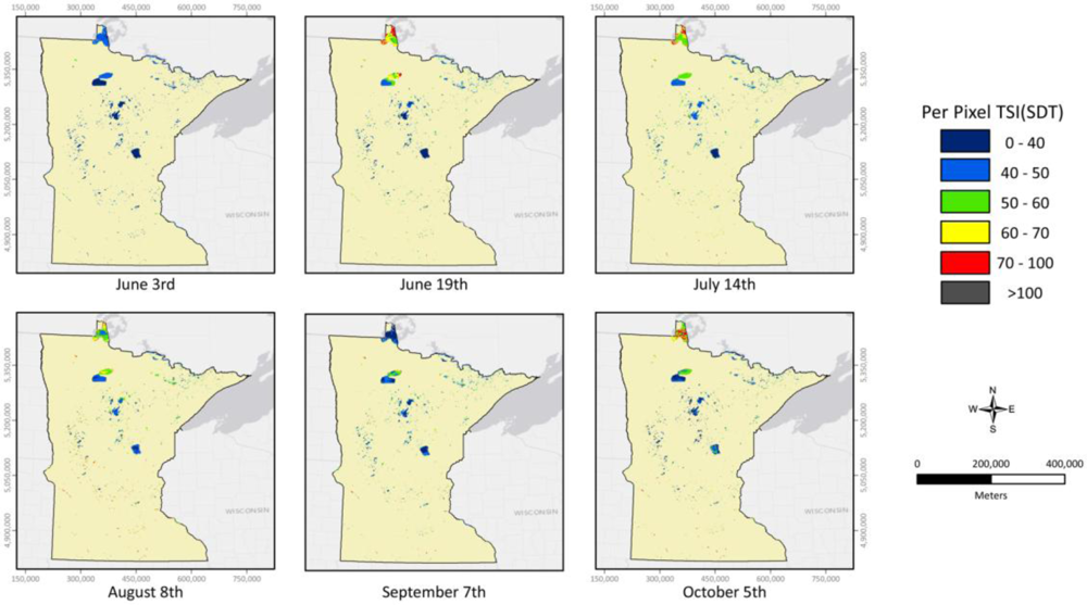
The regression equations were applied to the corresponding MODIS red and blue band layers to create per-pixel SDT layers for each image date. Water clarity maps depicting MODIS-predicted TSI (referred to as TSI(SDT)) for each date were similarly generated from the SDT layers using the TSI equations described above (Figure 1). Zonal statistics were computed to provide lake-average SDT and TSI(SDT) values for comparison to published ecoregion water quality trends.
3. Results
3.1. Within-Lake Water Clarity Variation
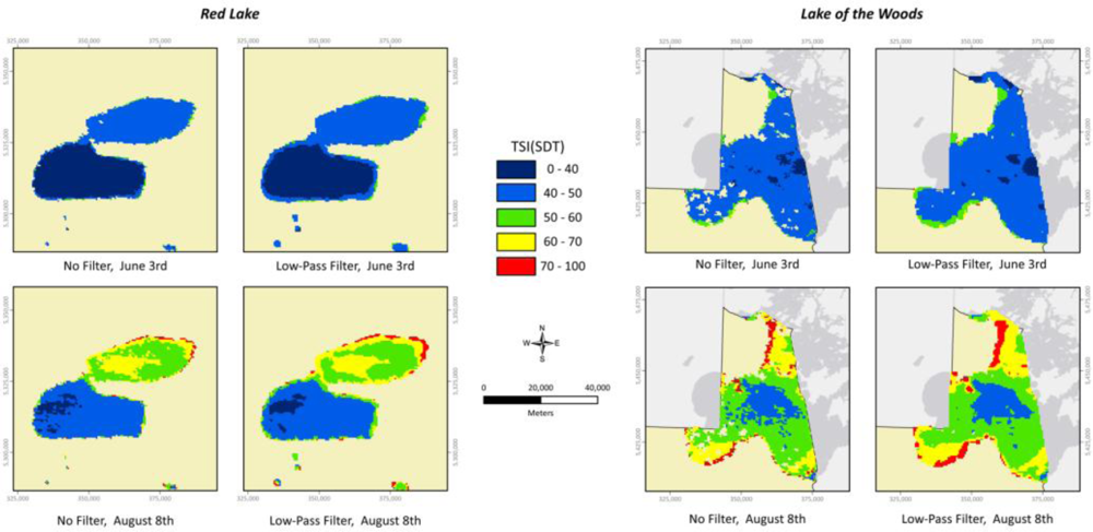
Lake water quality is not typically uniform, and variations in water quality are readily visible in water clarity estimates derived from satellite imagery as seen in Figures 1 and 2. Despite the relatively coarse MODIS spatial resolution, water clarity variations appeared around points of maximal water clarity in both Red Lake and Lake of the Woods. Red Lake in particular offers an example of a single lake with distinct bays exhibiting substantially different water clarity. The seasonal variation in water clarity exhibited by these two very large lakes is primarily due to land use pressures. Upper Red Lake is impacted by substantial agricultural drainage from the northwest, which creates algal turbidity as the growing season progresses. Lake of the Woods is impacted by runoff from urban development, agriculture, and forestry operations, which causes similar temporal variation in clarity. Spatial and temporal water clarity patterns were observed in other Minnesota lakes, though only large lakes showed internal water clarity variation.
3.2. Lake Averages by Date
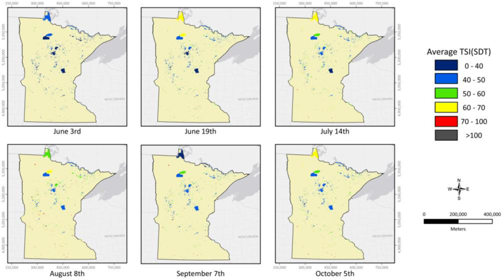
Per-pixel TSI estimates for the 434 lakes falling within the water mask (Figure 3) showed substantial spatial and temporal variability. In general, lakes with the highest water clarity estimates occurred in the north and north-east portions of Minnesota. In these portions of the state, land use impacts tend to be least. The north and north-east (“Arrowhead”) areas have much larger amounts of forests and both forested and non-forested wetlands relative to urban or agriculture. Lakes with lower TSI values typically occur in the west, south-west, and south-central portions of Minnesota. These areas are much more heavily impacted by land use practices such as agriculture and urbanization. Across the June to October temporal range of the study, water clarity in many lakes exhibited a strong downward trend. This trend is likely attributable to cessation of the spring thaw, sedimentation from agriculture fields and stream channels, increased anthropogenic nutrient inputs, and higher algal growth.
3.3. Accuracy Assessment
Accuracy assessments were conducted on the two image dates having over 40 CLMP points: 19 June (n = 50) and July 14 (n = 41). Half of the CLMP calibration points from each date were randomly selected to generate new regression equations. New SDT and TSI(SDT) layers were generated using the previously described procedures. The CLMP points not used to develop the regression for a given image date were compared against the TSI(SDT) values in the corresponding image pixels to assess the accuracy of the TSI(SDT) layer. This procedure was done twice for each scene, so that each subset of points was used both to develop the regressions and to assess them. The coefficients of determination, standard error, and range of SDT values exhibited by the point subsets are shown in Table 5.
After creation of the aforementioned validation dataset, two methods were used to assess the accuracy of the TSI(SDT) layers. First, all observed and predicted TSI(SDT) values were split into the four trophic state classes shown in Table 3. Matches between in situ measured trophic classes (calculated directly from CLMP point SDT) and predicted MODIS-derived trophic classes contributed to the trophic class accuracy (Table 6, Column 2). A second measure of the agreement between observed and predicted TSI(SDT) datasets involved quantifying the average distances in TSI(SDT) units between predicted and observed values (Table 6, Columns 3–6). This latter approach showed that overall, 18% of predicted TSI(SDT) values were within one TSI unit of their measured value, one-third were within 2 TSI, two-thirds within 5 TSI, and nearly all points fell within 10 TSI units.
3.4. Comparison of MODIS and Ground SDT Predictions
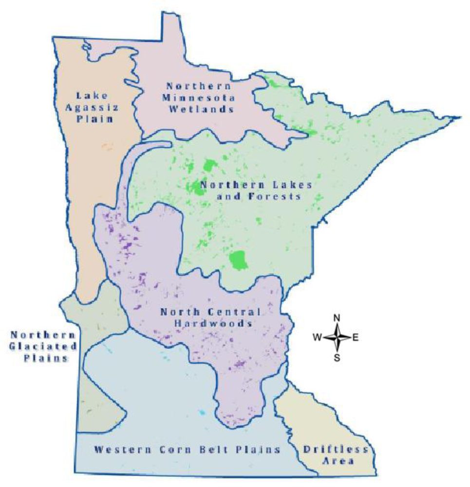
In Minnesota, MPCA hydrologists use the US EPA’s ecoregions to classify Minnesota lakes into seven categories (Figure 4) based on surrounding land use, current and/or potential vegetation, topography, hydrology, geology, and soils. Separating lakes by ecoregion allows policy makers and local water management agencies to set water quality standards for enforcement and rehabilitation purposes while keeping regulation appropriate to each region’s ecology. Ecoregions in Minnesota display different SDT patterns during the growing season [49–51].
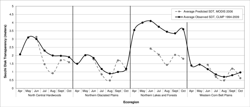
Four ecoregions in Minnesota contain 98% of the state’s lakes, while the other three ecoregions lacked sufficient in situ data for statistical analysis and were omitted from this study. Both the MODIS-predicted and observed CLMP SDT patterns exhibited the same high spring water clarity and midsummer decline (Figure 5). As expected, water clarity was at its seasonal lowest in August or September in each ecoregion [10,12].
MODIS-predicted 2006 SDT measurements were generally lower than the 25-year observed SDT average (Figure 5). Stadelmann et al. [10] noted that SDT in dry years often varies greatly from mean SDT. Since 2006 was a particularly dry year, reduced water clarity may be expected [46]. The Northern Lakes and Forests (NLF) and North Central Hardwood Forest (NCH) ecoregions were strongly affected by drought, though the influence was limited to July and August in the NCH and returned to more normal water clarity by late summer. The Western Corn Belt Plains (WCBP) ecoregion fell south of the severe drought region, and so exhibited more typical transparencies than other ecoregions.
MODIS-predicted SDT increased from early August to early September, and then decreased by early October. The October decrease in the NCH and NLF ecoregions may have corresponded to fall turnover stirring up lake sediments and causing lower SDT values, but the August to September increase in SDT, particularly such large increases (0.7 to 1.2 m), was unexpected. Temporal patterns of water clarity in Minnesota are characterized by seasonally low water transparency and minimal variation in transparency from 15 July to 15 September [10]. The CLMP’s average SDT depths collected over a 25-year period (1994–2009) showed minimal change in water clarity between August and September as well [52]. High August transparency may be due to high amounts of precipitation and flooding that occurred post-drought.
4. Discussion
4.1. Water Clarity Patterns
Both Kloiber et al. [19] and Scarpace et al. [53] acknowledged that within-lake water quality can be highly variable, but the typically used analysis procedure has been to average or normalize the values to the lake level rather than use that variation to describe local-level water quality issues or identify sources of sediment runoff. Monthly MODIS-derived SDT may provide important details on seasonal patterns for large lakes that can only otherwise be obtained through intensive monitoring programs. Differences between annual MODIS predicted SDT and multi-year averages of in situ collected SDT data, such as those presented in Figure 5, may also provide information on how large regional events such as flooding and drought effect short-term water clarity.
4.2. Regressions and Accuracy
The 3 June image’s particularly low coefficient of determination (R2) may have been due to image related factors such as haze or a high rate of change in water clarity during that time of year, since decreasing the SDT date window to within one day of satellite capture failed to improve the regression strength. Since many Landsat studies have focused on the mid-July to mid-September time period rather than examining lake clarity patterns throughout the summer, there is little other early summer research for comparison.
With the exception of 3 June, the remaining R2 values ranged from 0.51 to 0.71 and fell largely within the range observed by Kloiber et al. [12] in their multi-year Minnesota Landsat assessment. The 0.51–0.71 range is somewhat lower than those observed in other Minnesota studies (0.7–0.8 in Kloiber et al. [19] and 0.71–0.96 in Olmanson et al. [23], but higher than the 0.43 R2 value reported by Nelson et al. [16] in their Michigan study—though images of somewhat lower quality were used in the latter study [23]. Most studies reporting high R2 values used only mid-July to mid-September images, and so accounted for less variation in SDT in regression models.
Though water clarity studies often report R2 values and regression standard error, formal accuracy assessments are less common. However, as is shown in Tables 5 and 6, higher R2 values such as those observed in the 19 June-Subset 2 and 14 July-Subset 1 regressions did not necessarily result in a higher percentage of trophic class matches. Such findings suggest that R2 and standard error estimates may not be sufficient measures of accuracy for water clarity research. Those studies that do include accuracy assessments generally state the error rate relative to trophic state classifications and/or quantify the differences between predicted and measured TSI(SDT) values. Fuller and Minnerick [25] used both of these methods for a Landsat water clarity study in Michigan. The average agreement between observed and predicted trophic classes in the present study was 62%, somewhat lower than the 72% observed by Fuller and Minnerick [25]. Of their TSI(SDT) values, 42% were within 2 TSI units, 80% were within 5 TSI, and 98% fell within 10 TSI units. This study’s rates were again slightly lower, with 30% of values within 2 TSI, 67% within 5 TSI, and 93% within 10 TSI. Despite the substantial difference in spatial resolution, this study’s results compare well with those generated using Landsat imagery, in that MODIS data were suitable for predicting TSI(SDT) values similar to those of averaged in situ SDT. A limitation of this study is that each image date required a separate regression model. Attempts to create a single seasonal model for the study area using all valid in situ data were not successful. Similarly, the development of semi-analytical retrieval algorithms based on the optical properties of the many water bodies failed. We attribute these difficulties to the considerable spatial and temporal variation of clarity in the 434 studied lakes. Such variation consists of differences in the surrounding land cover/use types, physiographic influences (e.g., topography, soil type, vegetation), nutrient inputs, and size (extent and depth). Though constructing a model for each date is not ideal, the results of this study suggest that the approach can be used successfully to monitor lake clarity. We are unaware of an alternate approach, either empirical or semi-analytical, that can be used to construct a single seasonal model of water clarity for such a large number of highly variable lakes.
4.3. Bathymetry Data
The lake bathymetry data provided an efficient means by which to automatically remove areas likely to be composed of shallow water or land-lake boundaries. Using bathymetry information in this way was faster than a manual editing approach. However, while providing advantages in terms of speed, bathymetry data is not without disadvantages. First, bathymetry data may not be available for many lakes. Second, the user must select a depth threshold between deep and shallow water. This study used an empirically determined threshold of 2 m, but other values could be appropriate. Additionally, the optimal threshold may vary depending on local parameters such as lake size, depth, clarity, and depth variability. Finally, the results obtained from using bathymetry data are only as good as the accuracy of the bathymetry information itself. Validation information may not be available to aid in assessing the suitability of a given bathymetry dataset.
The results of this research suggest that future MODIS-based studies may yield stronger correlations if lake data is first separated by ecoregion, lake depth, and/or lake mixing frequency. Averaged lake TSI(SDT) values would also be more realistic if lake basins and bays were separated into smaller units based on patterns in the per-pixel SDT layers. Lakes such as Red Lake (shown in Figure 2) that exhibit significant spatial differences in water clarity may be better represented by averaging each distinct bay as a separate lake than by averaging such different values together. Such an effort would require manual editing of an existing lake boundary layer, but would only need to be completed once for the study area.
5. Conclusions
Water clarity estimates derived from calibrated MODIS scenes were demonstrated to be suitable for accurately describing the trophic states of inland lakes in Minnesota, as compared with field collected reference data. Such estimates fell with 10 TSI units of reference values, which represents good agreement. Though MODIS imagery cannot be used to observe the smaller lakes more readily resolved by Landsat imagery, MODIS is well suited to model both within-lake variation and average lake clarity on large lakes (>160 ha). This novel research suggests that MODIS’s frequent data acquisition provides an opportunity for repeated monitoring of large inland lakes, particularly when needed to track events such as sudden severe blue-green algae blooms or large-scale erosion and flooding. Further research is needed to identify image acquisition windows during the growing season and after severe events that are optimal for assessing changes in lake water clarity.
Acknowledgments
The authors gratefully acknowledge valuable assistance provided by Marvin E. Bauer and Leif G. Olmanson of the University of Minnesota. We also thank our peer reviewers and the editorial staff of Remote Sensing for their helpful comments. Funding for this research was provided by the University of Minnesota’s Grant-in-Aid program, the Department of Forest Resources, and the Agricultural Experiment Station.
References
- IPCC, Climate Change 2007: The Physical Science Basis. Contribution of Working Group I to the Fourth Assessment Report of the Intergovernmental Panel on Climate Change; Solomon, S.; Qin, D.; Manning, M.; Chen, Z.; Marquis, M.; Averyt, K.B.; Tignor, M.; Miller, H.L. (Eds.) Cambridge University Press: Cambridge, UK; p. 2007.
- Berkman, H.E.; Rabeni, C.F. Effect of siltation of stream fish communities. Environ. Biol. Fish 1987, 18, 285–294. [Google Scholar]
- Davies-Colley, R.J.; Smith, D.G. Turbidity, suspended sediment, and water clarity: A review. J. Am. Water Resour. Assoc 2001, 37, 1085–1101. [Google Scholar]
- De Robertis, A.; Ryer, C.H.; Veloza, A.; Brodeur, R.D. Differential effects of turbidity on prey consumption of piscivorous and plantivorous fish. Can. J. Fisheries Aquat. Sci 2003, 60, 1517–1526. [Google Scholar]
- Newcombe, C.P. Impact assessment model for clear water fishes exposed to excessively cloudy water. J. Am. Water Resour. Assoc 2003. [Google Scholar] [CrossRef]
- Walter, B.; Norman, R.; Brian, M.; Brian, H. The Biological Effects of Suspended and Bedded Sediment (SABS) in Aquatic Systems: A Review; Internal Report. USEPA: Washington, DC, USA, 2004. Available online: http://water.epa.gov/scitech/swguidance/standards/criteria/aqlife/pollutants/sediment/upload/2004_08_17_criteria_sediment_appendix1.pdf (accessed on 4 October 2011).
- Schwartz, J.S.; Dahle, M.; Robinson, R.B. Concentration-duration-frequency curves for stream turbidity: Possibilities for assessing biological impairment. J. Am. Water Resour. Assoc 2008, 44, 879–886. [Google Scholar]
- Lake Access. Turbidity in Lakes. Available online: http://lakeaccess.org/russ/turbidity.htm (accessed on 15 May 2012).
- Howard, D.M.; Minnesota Pollution Control Agency. Aquatic Life Water Quality Standards Draft Technical Support Document for Total Suspended Solids (Turbidity): Triennial Water Quality Standard Amendments to Minnesota Rules Chapters 7050 and 7052; Minnesota Pollution Control Agency: Saint Paul, MN, USA; p. 2011.
- Stadelmann, T.H.; Brezonik, P.L.; Kloiber, S. Seasonal patterns of chlorophyll a and Secchi disk transparency in lakes of East-Central Minnesota: Implications for design of ground- and satellite-based monitoring programs. Lake Reserv. Manag 2001, 17, 299–314. [Google Scholar]
- Minnesota Pollution Control Agency. Guide to Lake Protection and Management. Available online: http://www.pca.state.mn.us/publications/lakes-guide2-ch1-4.pdf (accessed on 15 May 2012).
- Kloiber, S.M.; Brezonik, P.L.; Bauer, M.E. Application of Landsat imagery to regional-scale assessments of lake clarity. Water Res 2002, 36, 4330–4340. [Google Scholar]
- Moore, G.K. Satellite remote sensing of water turbidity. Hydrolog. Sci.Bull 1980, 25, 407–421. [Google Scholar]
- Bukata, R.P.; Jerome, J.H.; Kondratyev, K.Y.; Pozdnaykov, D.V. Estimation of organic and inorganic matter in inland waters: Optical cross sections of Lakes Ontario and Ladoga. J. Great Lakes Res 1991, 17, 461–469. [Google Scholar]
- Bukata, R.P. Satellite Monitoring of Inland and Coastal Water Quality: Retrospection, Introspection and Future Directions; CRC Press: Boca Raton, FL, USA, 2005. [Google Scholar]
- Nelson, S.A.C.; Soranno, P.A.; Cheruvilil, K.S.; Batzli, S.A.; Skole, D.L. Regional assessment of lake water clarity using satellite remote sensing. J. Limnol 2003, 62, 27–32. [Google Scholar]
- Lathrop, R.G. Landsat thematic mapper monitoring of turbid inland water quality. Photogramm. Eng. Remote Sensing 1992, 58, 465–470. [Google Scholar]
- Cox, R.M.; Forsythe, R.D.; Vaughan, G.E.; Olmsted, L.L. Assessing water quality in the Catawba River reservoirs using Landsat Thematic Mapper satellite data. Lake Reserv. Manag 1998, 14, 405–416. [Google Scholar]
- Kloiber, S.M.; Brezonik, P.L.; Olmanson, L.G.; Bauer, M.E. A procedure for regional lake water clarity assessment using Landsat multispectral data. Remote Sens. Environ 2002, 82, 38–47. [Google Scholar]
- Menken, K.; Brezonik, P.L.; Bauer, M.E. Influence of chlorophyll and colored dissolved organic matter (CDOM) on lake reflectance spectra: Implications for measuring lake properties by remote sensing. Lake Reserv. Manag 2005, 22, 179–190. [Google Scholar]
- Lillesand, T.M; Johnson, W.L.; Deuell, R.L.; Lindstrom, O.M.; Meisner, D.E. Use of Landsat data to predict the trophic state of Minnesota lakes. Photogramm. Eng. Remote Sensing 1983, 49, 219–229. [Google Scholar]
- Olmanson, L.G.; Kloiber, S.M.; Bauer, M.E.; Brezonik, P.L. Image Processing Protocol for Regional Assessments of Lake Water Quality; Public Report Series #14; University of Minnesota: Saint Paul, MN, USA, 2001. [Google Scholar]
- Olmanson, L.G.; Bauer, M.E.; Brezonik, P.L. A 20-year Landsat water clarity census of Minnesota’s 10000 lakes. Remote Sens. Environ 2008, 112, 4086–4097. [Google Scholar]
- Peckham, S.D.; Lillesand, T.M. Detection of spatial and temporal trends in Wisconsin lake water clarity using Landsat-derived estimates of Secchi depth. Lake Reserv. Manag 2006, 22, 3331–3341. [Google Scholar]
- Fuller, L.M.; Minnerick, R.J. Predicting Water Quality by Relating Secchi-Disk Transparency and Chlorophyll A Measurements to Landsat Satellite Imagery for Michigan Inland Lakes, 2001–2006; Fact Sheet 2007–3022; US Geological Survey: Lansing, MI, USA, 2007. [Google Scholar]
- Fuller, L.M.; Jodoin, R.S.; Minnerick, R.J. Predicting Lake Trophic State by Relating Secchi-Disk Transparency Measurements to Landsat-Satellite Imagery for Michigan Inland Lakes, 2003–05 and 2007–08; Scientific Investigations Report 2011–5007; US Geological Survey: Lansing, MI, USA, 2011; p. 36. [Google Scholar]
- Binding, C.E.; Jerome, J.H.; Bukata, R.P.; Booty, W.G. Trends in water clarity of the Great Lakes from SeaWiFS and CZCS aquatic colour. J. Great Lakes Res 2007, 33, 828–841. [Google Scholar]
- Binding, C.E.; Jerome, J.H.; Booty, W.G.; Bukata, R.P. Spectral absorption properties of dissolved and particulate matter in Lake Erie. Remote Sens. Environ 2008, 112, 1702–1711. [Google Scholar]
- Binding, C.E.; Greenberg, T.A.; Jerome, J.H.; Bukata, R.P.; Letourneau, G. An assessment of MERIS algal products during an intense bloom in Lake of the Woods. J. Plankton Res 2010. [Google Scholar] [CrossRef]
- Binding, C.E.; Jerome, J.H.; Bukata, R.P.; Booty, W.G. Suspended particulate matter in Lake Erie derived from MODIS aquatic colour imagery. Int. J. Remote Sens 2010, 31, 5239–5255. [Google Scholar]
- Pozdnyakov, D.; Shuchman, R.; Korosov, A.; Hatt, C. Operational algorithm for the retrieval of water quality in the Great Lakes. Remote Sens. Environ 2005, 97, 352–370. [Google Scholar]
- Chen, Z.Q.; Hu, C.M.; Muller-Karger, F. Monitoring turbidity in Tampa Bay using MODIS. Remote Sens. Environ 2007, 109, 207–220. [Google Scholar]
- Becker, R.H.; Sultan, M.I.; Boyer, G.L.; Twiss, M.R.; Konopko, E. Mapping cyanobacterial blooms in the Great Lakes using MODIS. J. Great Lakes Res 2009, 35, 447–453. [Google Scholar]
- Werdell, P.J.; Bailey, S.W.; Franz, B.A.; Harding, L.W., Jr.; Feldman, G.C.; McClain, C.R. Regional and seasonal variability of chlorophyll a in Chesapeake Bay as observed by SeaWiFS and MODIS-Aqua. Remote Sens. Environ 2009, 113, 1319–1330. [Google Scholar]
- Horion, S.; Bergamino, N.; Stenuite, S.; Descy, J.-P.; Plisnier, P.-D.; Loiselle, S.A.; Cornet, Y. Optimized extraction of daily bio-optical time series derived from MODIS/Aqua imagery for Lake Tanganyika, Africa. Remote Sens. Environ 2010, 114, 781–791. [Google Scholar]
- Moreno-Madrinan, M.J.; Al-Hamdan, M.Z.; Rickman, D.L.; Muller-Karger, F.E. Using surface reflectance MODIS Terra product to estimate turbidity in Tampa Bay, Florida. Remote Sens 2010, 2, 2713–2728. [Google Scholar]
- Doron, M.; Babin, M.; Hembise, O.; Mangin, A.; Garnesson, P. Ocean transparency from space: Validation of algorithms estimating Secchi depth using MERIS, MODIS and SeaWiFS data. Remote Sens. Environ 2011, 115, 2986–3001. [Google Scholar]
- Miller, R.L.; Liu, C.-C.; Buonassissi, C.J.; Wu, A.M. A multi-sensor approach to examining the distribution of total suspended matter (TSM) in the Albemarle-Pamlico estuarine system, NC, USA. Remote Sens 2011, 3, 962–974. [Google Scholar]
- Olmanson, L.G.; Brezonik, P.L.; Bauer, M.E. Evaluation of medium to low resolution satellite imagery for regional lake water quality assessments. Water Resour. Res 2011, 47, W09515. [Google Scholar]
- USEPA, National Water Quality Inventory: Report to Congress, 2002 Reporting Cycle: Findings, Rivers and Streams, and Lakes, Ponds and Reservoirs; USEPA: Washington, DC, USA, 2007; Available online: http://water.epa.gov/lawsregs/guidance/cwa/305b/upload/2007_10_15_305b_2002report_report2002pt3.pdf (accessed on 4 October 2011).
- USEPA, National Water Quality Inventory: Report to Congress, 2004 Reporting Cycle: Findings; USEPA: Washington, DC, USA, 2004; Available online: http://www.epa.gov/owow/305b/2004report/report2004pt3.pdf (accessed on 4 October 2011).
- Minnesota Pollution Control Agency. Citizen Lake Monitoring Program Website. Available online: http://www.pca.state.mn.us/water/clmp.html (accessed on 15 May 2012).
- Anderson, P.; Heiskary, S. 2008 Lake Assessment Review Process Transparency Document. Available online: http://www.pca.state.mn.us/index.php/component/option,com_docman/task,doc_view/gid,8609 (accessed on 4 October 2011).
- Vermote, E.F.; Vermeulen, A. MODIS Algorithm Technical Background Document, Atmospheric Correction Algorithm: Spectral Reflectances (MOD09), Version 4.0. Available online: http://modis.gsfc.nasa.gov/data/atbd/atbd_mod08.pdf (accessed on 4 May 2012).
- Franz, B.A.; Kwiatkowska, E.J.; Meister, G.; McClain, C.R. Moderate resolution imaging spectroradiometer on terra: Limitations for ocean color applications. J. Appl. Remote Sens 2008, 2, 023525. [Google Scholar]
- State Climatology Office, DNR Waters. HydroClim Minnesota. Available online: http://climate.umn.edu/doc/journal/hc0609.htm (accessed 4 October 2011).
- Minnesota Pollution Control Agency. Citizen Lake-Monitoring Program: Instruction Manual. Available online: http://www.pca.state.mn.us/publications/wq-s1-13.pdf (accessed on 15 May 2012).
- Lake Access. TSI. Available online: http://lakeaccess.org/lakedata/datainfotsi.html (accessed on 15 May 2012).
- Heiskary, S.A.; Wilson, C.B.; Larsen, D.P. Analysis of regional patterns in lake water quality: Using ecoregions for lake management in Minnesota. Lake Reserv. Manag 1987, 3, 337–344. [Google Scholar]
- Heiskary, S.A.; Wilson, C.B. The regional nature of lake water quality across Minnesota: An analysis for improving resource management. J. Minn. Acad. Sci 1989, 55, 71–77. [Google Scholar]
- USEPA. Level III Ecoregions. Available online: http://www.epa.gov/wed/pages/ecoregions/level_iii.htm (accessed on 4 October 2011).
- Minnesota Pollution Control Agency. Lake and Water Quality. Available online: http://www.pca.state.mn.us/index.php/water/water-types-and-programs/surface-water/lakes/lakes-and-lake-monitoring-in-minnesota.html (accessed on 4 October 2011).
- Scarpace, F.L.; Holmquist, K.W.; Fisher, L.T. Landsat analysis of lake quality. Photogramm. Eng. Remote Sensing 1979, 45, 623–633. [Google Scholar]
Figure 1.
MODIS-predicted TSI(SDT) values per pixel in the statewide water mask. Significant within-lake water clarity variation is clearly visible in larger lakes. Seasonal progression in image dates is shown from left to right by row.
Figure 1.
MODIS-predicted TSI(SDT) values per pixel in the statewide water mask. Significant within-lake water clarity variation is clearly visible in larger lakes. Seasonal progression in image dates is shown from left to right by row.

Figure 2.
Within-lake TSI(SDT) variation, with and without low-pass filtering to smooth out variability in the maps. This image series includes examples from two of Minnesota’s largest lakes in MODIS images early in the growing season when lakes exhibit maximum clarity and later in the summer when lake clarity is at its seasonal low.

Figure 3.
Lake average TSI(SDT), averaged from the water pixels in each lake.

Figure 4.
US EPA ecoregion boundaries across Minnesota.

Figure 5.
Summer water clarity patterns, as predicted by MODIS imagery and observed by in-situ SDT data collected over a 25-year span. Higher Secchi depths correspond to higher water clarity. Note: 19 June MODIS predicted values were used for the “June” entry because mid-month values were assumed to be more typical than early month (3 June) values.


| 3 June | <10% Cloud and Haze |
| 19 June | <10% Cloud and Haze |
| 14 July | No Clouds or Haze |
| 8 August | <10% Cloud and Haze |
| 7 September | No Clouds or Haze |
| 5 October | No Clouds or Haze |
Table 2.
The number of Secchi disk transparency (SDT) points, the SDT point depth range, and the number of lakes used to calibrate the regressions for each MODIS image date.
| Image Date | Lake Count | SDT Point Count | SDT Range (m) |
|---|---|---|---|
| 3 June | 24 | 30 | 1.4–6.4 |
| 19 June | 35 | 50 | 1.5–8.2 |
| 14 July | 35 | 41 | 0.9–7.6 |
| 8 August | 25 | 26 | 0.8–7.9 |
| 7 September | 18 | 23 | 0.9–5.5 |
| 5 October | 21 | 22 | 0.8–7.3 |
| Lake Trophic State | Oligotrophic Lakes | Mesotrophic Lakes | Eutrophic Lakes | Hypereutrophic Lakes |
|---|---|---|---|---|
| Water Quality | Extremely High | Moderate | Poor | Extremely Poor |
| Photosynthetic Productivity (TSI) | Low (<30–40) | Intermediate (40–50) | High (50–70) | Extremely High (>70) |
| Nutrient Levels | Low | Intermediate | High | Extremely High |
| Typical Lake | Very clear, deep lakes | Seasonal algae blooms, various lake depths | Green water, shallow lakes | Green water, shallow lakes, summer blooms of blue-green algae (toxic) and surface scum |
| Secchi transparency | High | Intermediate | Low | Very low |
Table 4.
Regressions for each MODIS image date, shown with coefficient of determination and standard error.
| Image Date | Regression Equation | R2 | Standard Error |
|---|---|---|---|
| 3 June | ln(SDT) = (0.0086 × Band 3) − (0.0067 × Band 1) + 1.4451 | 0.32 | 0.31 |
| 19 June | ln(SDT) = (0.0155 × Band 3) − (0.0112 × Band 1) + 1.2812 | 0.66 | 0.26 |
| 14 July | ln(SDT) = (0.0087 × Band 3) − (0.0098 × Band 1) + 1.4751 | 0.67 | 0.33 |
| 8 August | ln(SDT) = (0.0111 × Band 3) − (0.0129 × Band 1) + 1.8579 | 0.51 | 0.48 |
| 7 September | ln(SDT) = (0.0155 × Band 3) − (0.0124 × Band 1) + 1.1711 | 0.71 | 0.27 |
| 5 October | ln(SDT) = (0.0086 × Band 3) − (0.0097 × Band 1) + 1.6895 | 0.62 | 0.36 |
Table 5.
June and July subset regressions, in which the SDT field sites available for each month were randomly split into two groups, with each group compared with regressions constructed using the other group.
| Image Date | R2 | Standard Error | Range SDT (m) |
|---|---|---|---|
| 19 June | |||
| Subset 1 (n = 25) | 0.63 | 0.28 | 1.5–8.2 |
| Subset 2 (n = 25) | 0.73 | 0.23 | 1.7–7.6 |
| 14 July | |||
| Subset 1 (n = 21) | 0.69 | 0.35 | 1.1–6.7 |
| Subset 2 (n = 20) | 0.67 | 0.32 | 0.9–7.6 |
Table 6.
Accuracy assessment of MODIS-predicted TSI(SDT), reported as percent trophic class accuracy and difference between observed and predicted TSI(SDT) values.
| Image Date | Trophic Class Accuracy | ±1 TSI | ±2 TSI | ±5 TSI | ±10 TSI |
|---|---|---|---|---|---|
| 19 June | |||||
| Subset 1 (n = 25) | 68% | 20% | 32% | 60% | 88% |
| Subset 2 (n = 25) | 64% | 16% | 24% | 68% | 92% |
| 19 June Average | 66% | 18% | 28% | 64% | 90% |
| 14 July | |||||
| Subset 1 (n = 21) | 52% | 19% | 29% | 67% | 90% |
| Subset 2 (n = 20) | 65% | 15% | 35% | 75% | 100% |
| 14 July Average | 59% | 17% | 32% | 71% | 95% |
| Overall Average | 62% | 18% | 30% | 67% | 93% |
Share and Cite
MDPI and ACS Style
Knight, J.F.; Voth, M.L. Application of MODIS Imagery for Intra-Annual Water Clarity Assessment of Minnesota Lakes. Remote Sens. 2012, 4, 2181-2198. https://doi.org/10.3390/rs4072181
AMA Style
Knight JF, Voth ML. Application of MODIS Imagery for Intra-Annual Water Clarity Assessment of Minnesota Lakes. Remote Sensing. 2012; 4(7):2181-2198. https://doi.org/10.3390/rs4072181
Chicago/Turabian StyleKnight, Joseph F., and Margaret L. Voth. 2012. "Application of MODIS Imagery for Intra-Annual Water Clarity Assessment of Minnesota Lakes" Remote Sensing 4, no. 7: 2181-2198. https://doi.org/10.3390/rs4072181