Article

An Approach to Mapping Forest Growth Stages in Queensland, Australia through Integration of ALOS PALSAR and Landsat Sensor Data

1
Institute of Geography and Earth Sciences, Aberystwyth University, Aberystwyth, Ceredigion SY23 3DB, UK
2
Queensland Herbarium, Queensland Department of Science, Information Technology, Innovation and the Arts, Brisbane Botanic Gardens Mt Coot-tha Rd Toowong, Brisbane, QLD 4066, Australia
3
Remote Sensing Centre, Queensland Department of Science, Information Technology, Innovation and the Arts, Ecosciences Precinct, 41 Boggo Road, Dutton Park, QLD 4102, Australia
4
School of Geography, Planning and Environmental Management, The University of Queensland, Brisbane, QLD 4072, Australia
5
School of Plant Biology, The University of Western Australia (M084), 35 Stirling Highway, Crawley, WA 6009, Australia
6
Tropical Research Institute (IICT), Travessa do Conde da Ribeira, 9 1300-142 Lisbon, Portugal
7
Department of Electrical Engineering, University of Southern California, Powell Hall of Engineering, 3737 Watt Way, Los Angeles, CA 90089, USA
*
Author to whom correspondence should be addressed.
Remote Sens. 2012, 4(8), 2236-2255; https://doi.org/10.3390/rs4082236
Submission received: 15 June 2012 / Revised: 24 July 2012 / Accepted: 24 July 2012 / Published: 2 August 2012
(This article belongs to the Special Issue Remote Sensing by Synthetic Aperture Radar Technology)

Abstract

:
Whilst extensive clearance of forests in the eastern Australian Brigalow Belt Bioregion (BBB) has occurred since European settlement, appropriate management of those that are regenerating can facilitate restoration of biomass (carbon) and biodiversity to levels typical of relatively undisturbed or remnant formations. However, maps of forests are different stages of regeneration are needed to facilitate restoration planning, including prevention of further re-clearing. Focusing on the Tara Downs subregion of the BBB and on forests with brigalow (Acacia harpophylla) as a component, this research establishes a method for differentiating and mapping early, intermediate and remnant growth stages from Japan Aerospace Exploration Agency (JAXA) Advanced Land Observing Satellite (ALOS) Phased-Array L-band Synthetic Aperture Radar (PALSAR) Fine Beam Dual (FBD) L-band HH- and HV-polarisation backscatter and Landsat-derived Foliage Projective Cover (FPC). Using inventory data collected from 74 plots, located in the Tara Downs subregion, forests were assigned to one of three regrowth stages based on their height and cover relative to that of undisturbed stands. The image data were then segmented into objects with each assigned to a growth stage by comparing the distributions of L-band HV and HH polarisation backscatter and FPC to that of reference distributions using a z-test. Comparison with independent assessments of growth stage, based on time-series analysis of aerial photography and SPOT images, established an overall accuracy of >70%, with this increasing to 90% when intermediate regrowth was excluded and only early-stage regrowth and remnant classes were considered. The proposed method can be adapted to respond to amendments to user-definitions of growth stage and, as regional mosaics of ALOS PALSAR and Landsat FPC are available for Queensland, has application across the state.

1. Introduction

Within the Brigalow Belt Bioregion (BBB) of Queensland and northern New South Wales, Australia, vegetated ecosystems with brigalow (Acacia harpophylla, F. Muell. ex Benth.) as a dominant, co-dominant (e.g., with belah; Casuarina cristata) or sub-dominant species were once widespread. However, since European settlement, the extent of forests regarded as remnant or relatively undisturbed has been reduced to <10% of their former range. As a result, all of the 12 Regional Ecosystems (REs) within the BBB with brigalow as a component are considered endangered [1]. Nevertheless, whilst clearing has been extensive, forests have also regenerated, particularly from the 1950s onwards, resulting in many approaching maturity (herein referred to as intermediate regrowth). Forests at the earliest stage of regrowth (typically <15 years) have also become more widespread following a substantial rise in clearance rates from the mid-1990s and early 2000s and subsequent restrictions on vegetation clearance following the Vegetation Management Act (VMA; [2]), which aimed to phase out the broad scale clearing of remnant vegetation by the end of 2006, and a moratorium on clearing of regrowth vegetation in 2009. The extent of forest clearance was also so large that many landholders were unable to retain the land in agriculture.
The regeneration of forests with brigalow has been unwelcome by many, largely because the potential for stocking and establishing crops and pastures is compromised [3]. However, the importance of regrowth is becoming increasingly recognised as it represents the primary mechanism for restoring endangered and vulnerable regional ecosystems, including those containing brigalow [4,5]. Ecosystems with brigalow as a component also support stocks of biomass and biomass accumulation rates that are often higher compared to woody vegetation in similar climatic zones [5]. Hence, these systems offer significant potential for sequestering carbon [4] and, through increased diversification of habitat structures, restoring biodiversity [6,7]. However, appropriate management strategies (e.g., thinning [5,8], weed control) need to be put in place to encourage recovery of the brigalow ecosystems and minimise potentially irreparable damage to ecosystem function. The implementation of such strategies requires knowledge of the spatial distribution of forests at different stages of structural development, particularly when prioritising for biodiversity values.
To estimate the age and extent of regrowing vegetation, time-series of remote sensing data (e.g., historical aerial photography [6] or satellite data [9]) have previously been used. For example, time-series of Landsat-derived Foliage Projected Cover (FPC) data, which are available annually from 1988 [10], have been exploited to map regrowth (e.g., [4,8]), although only on land cleared within the last 25 years. However, estimates of forest age derived from remote sensing data may be compromised by gaps in the time-series (e.g., due to cloud cover) and do not always provide a consistent indicator of growth stage, particularly as the structural development of forests varies as a function of, for example, clearing histories, soils and climate. As an alternative, stages of structural development may be considered. However, discrimination using optical data alone is difficult as derived measures (e.g., Normalised Difference Vegetation Index; NDVI [11] or FPC [12]) for regrowing stands rapidly approach that of undisturbed forest as the canopy cover increases, making discrimination between mature forests and the earlier stages of regeneration difficult. By contrast, active sensors such as Light Detection and Ranging (LiDAR) and Synthetic Aperture Radar (SAR) data, particularly when acquired at longer wavelengths (i.e., L- (∼25 cm) and P-band (∼70 cm)), provide more information on the woody structure of vegetation which takes longer to recover following disturbance. Such sensors can be used to retrieve structural parameters (e.g., height from LiDAR or SAR interferometry [1316]) or estimate biomass (e.g., [1719]), which can be related to regrowth stage. Alternatively, classification approaches may be used to estimate regrowth stage directly from remote sensing data (e.g., [20]) although these rely on differences in the spectral and/or scattering characteristics of each. As an approach to mapping brigalow regrowth, Lucas et al. [12] proposed the combination of L-band SAR and Landsat-derived FPC, with capability demonstrated for a small area (near Injune in central southeast Queensland) using polarimetric airborne SAR (AIRSAR) data.
The launch of the Japan Aerospace Exploration Agency (JAXA) Advanced Land Observing Satellite (ALOS) Phased-Array L-band SAR (PALSAR) in 2006 offered an opportunity for forest mapping across wider areas, particularly given that dual polarisation (HH and HV) mosaics were subsequently made available for larger regions, including Australia and Central Africa [21]. Furthermore, as these datasets were progressively analysed, the benefits of using a combination of optical and PALSAR data rather than either alone became increasingly evident (e.g., for forest/non-forest discrimination; [22]). The availability of ALOS PALSAR data across the BBB also provided the opportunity to evaluate the combination of FPC and L-band SAR for discriminating and mapping brigalow regrowth proposed by Lucas et al. [12], which was the focus of this study. More specifically, the aims were to establish whether:
  • In addition to early-stage regrowth, remnant (mature) and intermediate stages with brigalow as a component could be differentiated using ALOS PALSAR data in combination with Landsat-derived FPC.
  • Acceptable accuracies for mapping regrowth extent and progressive stages of structural development could be achieved, with potential application across the entire BBB.
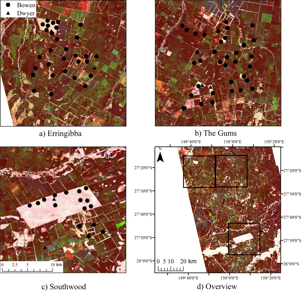
The paper is structured as follows. The introduction has provided a background to the study whilst Section 2 describes the study area which is located within the Tara Downs subregion of the BBB. Section 3 outlines the field and remote sensing data available for the study. Following an overview of the structural characteristics of forests dominated by brigalow and at different stages of structural development, Section 4 outlines the methods used to define growth stages, first from field-based measurements and subsequently from the ALOS PALSAR and Landsat FPC data. The maps of regrowth stage together with estimates of classification accuracy are then provided in Section 5 The approach to classifying regrowth stage using these combined datasets is then discussed in Section 6 and the study is concluded in Section 7.

2. Study Site

The study focused on an area of the Tara Downs subregion, located in the Western Darling Downs (27°16′S, 149°40′E to 27°52′S, 150°13′E) and contained within the southern Brigalow Belt. The subregion incorporates Southwood National Park, at 7,300 ha the largest remnant brigalow forest within the region [6]. Over 90% of the previously forested land has been converted to pasture and cereal crops and the remaining forests are typically located in narrow strips within a highly fragmented landscape. Forests with brigalow as a component are largely associated with Regional Ecosystem (RE) 11.4.3, although other REs include 11.4.7, 11.4.10, 11.3.1 and 11.9.5 [23]. A description of each RE is provided in Table 1.

3. Available Data

3.1. Field Data

Within the Tara Downs subregion, field data had been collected by Bowen et al. [6] and Dwyer et al. [7] between 2005 and 2007. In the latter case, only eight plots were located within the study area with the remainder distributed throughout the BBB. The locations of field plots are illustrated in Figure 1. Bowen et al. [6] measured stands of brigalow and belah at 82 sites, all within RE 11.4.3. The sites were located at Erringibaa (31; Figure 1(a)), The Gums (35; Figure 1(b)) and Southwood National Park (16; Figure 1(c)) respectively, with patch area within contiguous brigalow communities ranging from 2.2 to 2,600 ha. At each site, 4 × 50 m transects were positioned from 25–75 m and 125–175 m along a 200 m transect although, where stands were limited in area or dimension, the transect length was reduced to <50 m. Within each transect, the diameter at breast height (DBH) of all live and dead trees (1.5 m in height and not branching from the base) was recorded. Shrubs (including brigalow) <1.5 m in height were counted. The start and end distance of crowns (both trees and shrubs) that directly intersected the mid-line of the transect (above or below the measuring tape) were also recorded to allow subsequent estimation of canopy cover (%). At 10 m intervals along each 50 m transect, the height of trees was measured, with separate measurements recorded for emergents, the canopy, sub-canopy, low trees and both tall and low shrubs. Only those plots for which canopy measurements ware available were considered. Sampling was conducted during two survey periods from September 2005 to February 2006 and June to August 2006. Dwyer et al. [7] collected data from 55 sites where brigalow was dominant or co-dominant within the regenerating forest community, with eight located within the Tara Downs subregion, all of which were within within RE 11.4.3. At each site, data were collected from up to four 50 × 4 m transects (at least 50 m apart), with the transect width depending upon the density of stems. Within each transect, the diameter of each stem (including those associated with multi-stemmed individuals) was measured at the base and for all stems >2 cm. As with Bowen et al. [6], canopy, shrub and ground cover were recorded at 2 m intervals along each transect using the point intercept method as well as the height of canopy trees. Sampling was undertaken between September and November 2007, with this commencing in the south of the study area and progressing north.

3.2. Remote Sensing Data

For sites associated with field data and located within the Tara Downs, two ALOS PALSAR scenes were acquired on 26 September 2008 in Fine Beam Dual (FBD) mode; HH- and HV-polarisation, with a look angle of 34.3°. These data were provided as part of the JAXA Kyoto and Carbon (K&C) Initiative in level 1.0 format and were processed using the GAMMA Remote Sensing and Consulting AG (GAMMA) software package [24,25]. Data were processed to single-look complex (SLC) using the GAMMA Modular SAR Processor (MSP; [24]). Georeferencing to an UTM coordinate system, and resampling to a 12.5 m ground resolution, was undertaken using the GAMMA DIFF & GEO package [25], following the method described in Armston et al. [26]. For initial positioning, orbital data and topographic information from a 30 m resolution SRTM-derived Digital Elevation Model (DEM; [27]) were used. For each scene, a subset of the DEM was taken and resampled to 12.5 m using a bilinear interpolation. Positioning was refined using Ground Control Points (GCPs) generated initially from SAR data simulated from the DEM and subsequently, from the panchromatic band of Landsat ETM+ data (resampled from 15 m to 12.5 m spatial resolution). A RMSE of < 1 pixel was obtained in both range and azimuth. Finally, using the SRTM-derived DEM, topographic normalisation of the data was undertaken by first adjusting for distortions in pixel area as a function of slope and then correcting to a reference value associated with the incidence angle at mid-swath for flat terrain [28].
For the study area, Landsat FPC data were generated as part of the Statewide Landcover and Trees Study (SLATS) program and using standardised procedures outlined by Danaher et al. [29] and Armston et al. [10]. FPC is the percentage of ground area covered by the vertical projection of photosynthetic vegetation and is measured in the field using point-transect intercepts. FPC is calculated from Landsat bands 2–7 and Vapour Pressure Deficit (VPD) data using a multiple linear regression model [10]. Based on cross-validation and comparison with independent LiDAR-derived estimates of FPC, the regression model provided an adjusted R2 of 0.80 and RMSE of <10%. Trend analysis for time-series FPC estimates were used to separate woody from herbaceous FPC and produce annual FPC estimates. Composites of Landsat derived FPC and ALOS PALSAR HH and HV data are shown in Figure 1.

4. Methods

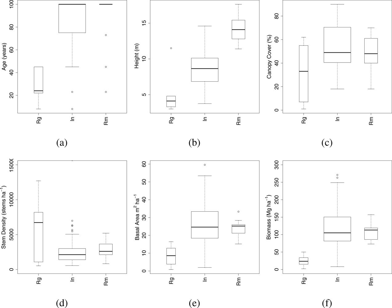
4.1. Structural Characteristics of Regrowth Stages

For classification, three stages of regrowth (early, intermediate and mature or remnant) were targeted. Remnant vegetation may be described using, for example, age, floristic characteristics and/or structural attributes. In Queensland, regenerating vegetation is considered remnant once it has attained 70% of the height and 50% of the Canopy Cover (CC) relative to that of the undisturbed stratum, with this defined as one that shows no evidence of extensive mechanical or chemical disturbance and is similar in terms of plant species composition [30]. The cover and height of the undisturbed (remnant) stratum is defined through the use of reference, or Core Vegetation (CORVEG) sites, information on which is contained within the Queensland Herbarium’s ecological site database. For other forests to be associated with a reference site, they have to be on the same landform (i.e., described by soil type and geology; [30]).
Within the Tara Downs study area, the majority of brigalow regrowth was classified as RE 11.4.3. Therefore, only plots within this RE were considered when developing an approach to differentiating regrowth stages. Based on biocondition reports [31], the reference height (href) and CC (CCref) for this RE were set to 24 m and 70% respectively. Regrowth stage was defined relative to these and forests were considered to be remnant if they supported at least 70% of the height (0.7href) and 50% of the CC (0.5CCref) of these reference sites. An existing definition of early-stage and intermediate regrowth was not available. Therefore, values of 0.3href and 0.3CCref were defined for early-stage regrowth, with the intermediate growth stage considered to lie between early stage and remnant vegetation.
On this basis, the 74 available field plots within RE 11.4.3 were separated into early-stage (6), intermediate (13) and remnant (55), with this based on their measured canopy cover and maximum height relative to that of the reference values. For each field plot, a prior indication of age class and structure was obtained through reference to field measurements and associated field-based classifications, with the latter based on interviews with landholders, and estimates of forest age generated through time-series comparison of aerial photography and satellite sensor data. In terms of estimated age (Figure 2(a)), all three stages of growth were separated (most plots classified as remnant were assigned an age of 100 years, with this corresponding to no record of clearing). Of the structural attributes considered, height (Figure 2(b)) provided a better indicator of the stage of development as regrowth stands rapidly attain a canopy cover that exceeds 40% and typically remains at or above this level up to maturity (Figure 2(c)). Early-stage regrowth was characterised by a high density of stems of small diameter, with these collectively supporting a canopy cover that approached that of intermediate regrowth and remnant forest (Figure 2(d)). Thereafter, stem density progressively decreased being least within the remnant forests. Basal area (BA; Figure 2(e)) and biomass (Figure 2(f)) were similar for intermediate and remnant vegetation, with a greater variation observed for intermediate regrowth.

4.2. Characterising Regrowth from Remote Sensing Data

To investigate relationships with field-based estimates of stand structure, Landsat-derived FPC and ALOS PALSAR backscatter were extracted from the locations associated with the site rather than the transect locations. These were selected as the greater area enabled averaging over a larger number of pixels to reduce random noise (e.g., that associated with speckle in the SAR data). Typically, values were extracted from areas greater than ∼50 pixels, with these varying with the size of the polygons associated with each plot.
Using the extracted data, the significance of differences between the L-band HH and HV backscatter and Landsat FPC data distributions for each growth stage was determined using a two-sample Welch t-test [32], with the normality of distributions confirmed using a Kolmogorov–Smirnov test [33]. The t-test showed the HH- and HV-polarisation backscatter of early stage regrowth to be significantly different from both the intermediate and remnant classes in all channels (p < 0.01) but the difference between the intermediate and remnant stages was less significant (p < 0.05) for both HH- and HV-polarisation data (∼39° incidence angle). Differences between FPC for intermediate and remnant classes were not found to be significant.
Differences in L-band backscatter observed for the different stages of regrowth were attributed to changes in scattering mechanism, with these linked to the structural development of the forest. In the earliest stages of regrowth, stems of high density are often of insufficient size to evoke a strong response at L-band [12]. Hence, ground scattering away from the sensor dominated, with this leading to a low backscatter return at both HH- and HV- polarisation. However, as the stands developed, stems become sufficiently large for double-bounce scattering to occur, with this leading to a larger response, particularly at HH-polarisation. The increasing amount of woody material in the canopy also leads to an increase in volume scattering and an associated HV-response. Within the more advanced stages of growth (primarily remnant), the comparatively greater amount of trunk and branch material results in an HH and HV backscatter (resulting primarily from double-bounce and volume scattering respectively) that is collectively greater than that observed within the younger counterparts. These observed differences in scattering mechanisms provided a basis for the discrimination and classification of regrowth stage.

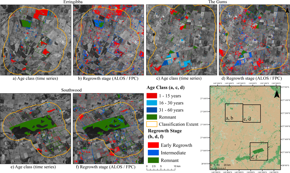
4.3. Approach to Regrowth Mapping

To map the different stages of regrowth across two images acquired over the Tara Downs subregion, an object-based approach was implemented. Objects were generated using a “multi-resolution” segmentation algorithm within eCognition [34], with equal weighting given to the ALOS PALSAR FBD and Landsat FPC data. Prior to segmentation, a 5 × 5 Lee filter [35] was applied to the HH and HV data to reduce speckle, and pixel values were expressed in dB. Visual comparison with aerial photography suggested that the combination of Lee-filtered SAR data and FPC generated segments that were broadly representative of the distribution of different forest types and non-forest. The segmentation was also undertaken such that the majority of objects contained more than 30 pixels.. The unfiltered data (in linear units) were retained at the object level to ensure correct averaging.
Once segmented, the distributions of L-band HH and HV and Landsat FPC data for each object were compared to reference distributions associated with each of the three stages of regrowth, as determined previously through reference to field data. As objects typically contained more than 30 pixels, the significance of difference between the object and reference distributions in each of the three channels was established using a z-test rather than a t-test, for computational simplicity. The z-score for each object was defined as:
z i , d = σ ¯ i , d σ ¯ o b , d SE i , d 2 + SE o b , d 2
where σ̄i,d denotes the mean value for class (i) in channel d and σ̄ob,d the mean value of the object in the same channel. The standard error on the mean (SEi,d for the class and SEob,d for the object) is given as:
SE d = υ d N
where vd is the standard deviation on the mean and N is the sample size, taken as the number of plots for the class or pixels within the object. The z-test allows each object to be assigned a class based on the significance of difference from reference distributions. Whilst supervised pixel-based classifiers, such as maximum-likelihood, also rely on finding the difference of each pixel to a test class and may be applied on an object basis, the use of a z-test allows the standard error of each object to be included in the classification, thereby accounting for object size and within-object variance. The classification can also be performed sequentially, such that objects in between already-assigned classes may be assigned to an appropriate transitional class (such as intermediate) rather than being left unclassified. Different thresholds of the resulting z-scores can also be used to determine the assignment of objects to a regrowth stage, with these based on, for example, knowledge of microwave scattering processes or ecology.
The approach to classification of the regrowth stages based on significant difference was evaluated for forests associated with RE 11.4.3 as the majority of field data had been collected from this RE. First, the extent of forests, regardless of their growth stage, was mapped by applying an FPC threshold of 9%, thereby allowing separation from non-forest (as used in [20]). A z-test was performed between the distributions of each object and the reference, such that zi,d was calculated for each channel (d) to give the difference of the object mean compared to that of regrowth (denoted zRg,d), intermediate (zIn,d) and remnant (zRm,d). The following rules were then used to assign each object to one of three classes with these being:
  • Early-stage The backscatter of the object was not significantly greater than that of early-stage regrowth at HH- and HV-polarisation (zRg,HH < 2∩zRg,HV < 2), with this corresponding to the area shaded red in Figure 3.
  • Remnant The backscatter of the object was not significantly less than that of remnant vegetation at HH- and HV-polarisation (zRm,HH > −2 ∩ zRm,HV > −2), with this corresponding to the area shaded green in Figure 3.
  • Intermediate Assigned to all objects not classified as regrowth or remnant, with this corresponding to the area shaded blue in Figure 3.
The distribution of backscatter values within each class is shown in Figure 3. Whilst there is an overlap between classes, errors within the intermediate class were considered acceptable as long as the remnant and early stage vegetation were classified correctly. The identification of remnant forest is particularly important as these represent the most intact and mature ecosystems with the highest carbon and often biodiversity values. Early-stage regrowth represent forests that can potentially be preserved into the future but which are arguably the most vulnerable because of their relative ease of clearance compared to older forests.
To evaluate the approach to classification using z-scores, with respect to existing classifications, a map of regrowth stages was also generated using the maximum-likelihood classification. Although a number of techniques exist for classifying remote sensing data, the maximum-likelihood classification was chosen as it is a well established technique and also includes the variance of the training samples. To enable comparison with the z-scores technique, the classification was applied at the object level, using the same objects used for the z-scores classification. For each object, the likelihood for a class (gi) was calculated using [36]:
g i = ln | C i | ( σ ¯ o b σ ¯ i ) t C i 1 ( σ ¯ o b σ ¯ i )
where σ̄ob is the vector of mean FPC and HH- and HV-polarisation backscatter for each object, σ̄i is the mean vector for the comparison regrowth stage and Ci, is the covariance matrix for the regrowth stage. Both σ̄i and Ci were estimated using values extracted from field plots (as with the significance classification). Each object was assigned the class with the maximum-likelihood.

5. Results

The classifications of regrowth stages for Erringibba, the Gums and Southwood are provided in Figure 4. In each case, the maps are compared with a classification generated by [6] through time-series comparison of aerial photography and SPOT High Resolution Geometric (HRG) data and with reference to field survey and landholder interviews. As the last image in the time-series used by [6] was acquired in 2005, the maps were updated by (a) only considering polygons with an average FPC in 2009 of >9% and (b) adding three more years to the age of regrowth and reclassifying areas into the age groups of <15 years, 15–30 years, 30–60 year and remnant, as defined by [6]. The adjusted classification is shown in Figure 4.

5.1. Validation

To assess the accuracy of the classification, the adjusted forest age class map of [6] was used. For comparison, the age classes of 15–30 and 30–60 years were together assigned to an intermediate regrowth class whilst the early regrowth forests were associated with forests estimated to be up to 15 years of age. All forests older than 60 years were assumed to be remnant. Both classes were compared within intersecting areas. To account for the differences in polygon sizes the area of the intersect was used rather than a count of each class. Confusion matrices for both the significance-based and maximum-likelihood classifications (Table 2) confirmed overall accuracies of 72% and 73% respectively. In both cases, the low overall accuracy was attributable to early regrowth forests being classified as 16–60 year old regrowth and remnant (>60 year old) forests being classified as 16–60 year old regrowth forest. When the forests mapped by Bowen et al. [6] were re-classified into young (< 30 years) and old regrowth / mature forest (>30 years) and compared to early-stage and remnant classes, the classification accuracy using both the significance-based and maximum likelihood classification increased to 90%.
The age class map derived from the time-series of aerial photography and satellite data [6] was not a classification of structural forms. Therefore, some of the errors in the classification were attributed to the variability in the structure of forests because of natural and anthropogenic influences (e.g., soil type, disturbance regimes). To provide some insight into this variability, the proportion of each growth stage within each year following clearing is given in Figure 5. In general, a higher percentage of areas classified as early regrowth were associated with the younger forests whilst those classified as intermediate and remnant forests were associated with the older regrowth and mature forest. Within the field data used for training the classification, a wide range of age classes was observed for both intermediate (8–100 years) and remnant forest (23–100 years), indicating the variability of ages within a single structural class.

6. Discussion

Many approaches to defining and mapping of growth stage have been developed, both from a ground and earth observation perspective. Even so, in each case, the difficulty in defining the stage of growth increases with the structural heterogeneity of the forests. For example, within natural forests where natural succession occurs in response to disturbance regimes or natural dieback, individual trees at various stages of growth occur and hence a discrete growth stage often cannot be assigned. However, where plantations occur or forests are establishing on cleared land, relatively homogeneous even-aged stands of forests are more common and their age can be estimated through reference to, for example, measures of structure (e.g., height or biomass; [37]), planting records or time-series of satellite sensor data (e.g., [9]). However, forests of similar age can be very different in terms of their structure and accumulated biomass, partly because of influencing factors such as local growth conditions as a function of soils, climate and topography or natural or human-induced events and processes (e.g., fire, drought or prior land use history). Forests dominated by brigalow and regrowing on land cleared previously for agriculture are a case in point, as these may remain as a low stature (typically <5 m) and structurally similar form (e.g., in terms of height and cover) over periods exceeding forty years, as individuals do not have the resources to out-compete others in what is often a high-density forest. Hence, practices such as restoration thinning are needed for succession to proceed [5]. For other brigalow forests, growth is less restricted and gains in height over the same period are greater. For these reasons, and as highlighted in this study, definitions of regrowth stage need to consider the structural development of the forests with this based on relative or actual differences in, for example, retrieved cover, height, density and/or biomass relative to that of undisturbed mature (or remnant) forest of the same community composition and occurring on the same landform (with similar soils, geology and topography).
Defining growth stage relative to the mature state requires identification and measurement of these forests for different ecosystems. Within Queensland, the structural development of stands is determined by considering field measures of height and cover relative to undisturbed stands. The approach adopted in this study mirrors this method to classify available field data but with a new definition of the early regrowth stage included (i.e., 30% of height and cover relative to undisturbed stands) and intermediate stages defined as the transition between the early-stage and remnant vegetation. Whilst set in this study, the 30% threshold can also be amended depending upon user-definitions of regrowth stage, with this being one of the benefits of the approach developed here.
The identification of reference sites is an essential component of the method and allows the mapping of growth stage to be progressively refined as more field data become available and a better understanding of the structural changes that occur as the forests regenerate and their manifestation within the remote sensing data is obtained. The study therefore advocates the establishment of reference sites and associated measurements across the range of REs occurring within the BBB but also other bioregions throughout Queensland. A particular advantage of the approach is that there is no requirement to establish empirical relationships between the ALOS PALSAR L-band SAR data and biophysical attributes (e.g., biomass) when defining growth stage. Instead, the HH and HV response is assumed to effectively summarise the relative amounts and characteristics of plant material (as a function of their size, density, geometry and moisture content) which can then be used subsequently to facilitate discrimination of regrowth stage, particularly if the additional information from the FPC layer is integrated.
The approach to mapping the three stages of brigalow regrowth is also based on an understanding of microwave interaction with different structural elements of the forests and particularly differences in the scattering mechanisms that occur. As forests regenerate on previously cleared land, there is a progression from ground scattering away from the sensor to double-bounce scattering at HH polarisation from the stems as these attain a size that is sufficient to evoke a response. The corresponding increase in volume scattering at HV-polarisation also reflects the increase in the size and density of plant (woody) material within the canopy. Within the remnant forests, the canopy cover is typically towards the maximum attainable by the stand and the biomass level is above that at which saturation of the HH and HV backscatter typically occurs, with this reflecting the high contributions from double-bounce and volume scattering. Hence, these forests collectively exhibit a high backscatter at both polarisations and also FPC. Forests at intermediate stages of growth are associated with increasing HH and HV backscatter and FPC as these transition to the remnant state. The response of these forests is more variable compared to the early regrowth and remnant forests and hence when only the latter were considered, the accuracies of classification were greater.
The statistical significance-based classification, using a z-test, represents an improvement on simple thresholding (e.g., [12]) and the benefits of a rule-based sequential classification are maintained. Compared to the significance-based classification, slightly higher but comparable levels of accuracy were observed when a maximum-likelihood classification algorithm was applied. The strong performance of this algorithm was attributed, in part, to the classification being performed at the object level, which reduced some of the noise present compared to when applied at the pixel level and also the relative simplicity of the rule-based approach to growth stage classification.
For this study, only a single RE was considered (11.4.3) whereas within the BBB, 12 REs with brigalow as a component occur. For several of these, different reference values for height and cover have been defined [31] and hence, in principal, different reference values of FPC and both L-band HH and HV data are needed. Furthermore, within a single RE, variations in the structure of undisturbed stands may occur, as in the case of RE 11.4.7 and 11.9.5, where the median canopy height for remnant stands varies from 16–25 m and 14–18 m across a rainfall and temperature gradient from the western interior to the eastern coastal margins. Consideration therefore needs to be given to climate and also soil gradients as well as local variations in, for example, slope, aspect and elevation.
In summary, the method presented is well suited to mapping the different growth stages of forests where brigalow is a component in that:
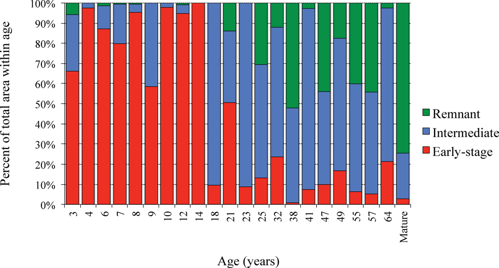
  • Regenerating forests may remain “locked-up” for many decades before events (e.g., fire or thinning) allow structural development to occur; hence, older forests may have similar characteristics as young regrowth which leads to age being an unreliable indicator of growth stage.
  • Reference distributions for each channel can be adapted depending on the users definition of growth stage.
  • The thresholds chosen for the z-scores can be varied to reduce commission or omission errors, based on mapping requirements. Whilst the same is true of backscatter thresholds, the use of z-scores considers the probability that the object is part of the same reference distribution.

7. Summary and Conclusions

Since European settlement, the extent of forests with brigalow as a component has been reduced such that only 10% are currently regarded as remnant, with these often being fragmented. The diverse history of land use throughout the Brigalow Belt Bioregion (BBB) has resulted in forests at various stages of regeneration, with these typically establishing on abandoned agricultural land. Focusing on the Tara Downs subregion of the BBB, this study has demonstrated that three stages of regrowth can be discriminated by considering differences in the Advanced Land Observing Satellite (ALOS) Phased-Array L-band Synthetic Aperture Radar (PALSAR) L-band HH and HV backscatter and Landsat Foliage Projective Cover (FPC) distributions extracted from objects defined from the image data relative to those from known areas of remnant forest. Early-stage regrowth forests were similarly discriminated, with all remaining areas associated with intermediate stages of regrowth.
The method represents an advancement on previous techniques for mapping brigalow regrowth that have been based solely on the use of Landsat FPC data, with these acquired in a single year or over several years (e.g., [8]), as the L-band SAR data allows information on the woody component of regrowth to be incorporated into the classification. The method proposed also represents an improvement on previous studies [12,20] that have combined L-band SAR and FPC through the use of simple thresholds. Although these studies also utilised knowledge of scattering mechanisms to differentiate one or several regrowth stages, the method developed here instead used field data to identify these stages and generate reference distributions for FPC, L-band HH and HV data. The distribution of backscatter values, within an image object, was compared to these reference distributions using a z-test, hence the probability that an object is part of the same reference distribution, and thus the same regrowth stage, was considered. These reference distributions can be adapted depending on the users’ definitions of growth stage and available field data. Accuracies in the classification exceeded 70% when the three stages of regrowth were considered, with this increasing to 90% when only two were mapped. The levels of accuracy were comparable to those generated using an object-based maximum-likelihood classification, although the proposed method was more easily implemented and interpretable.
The approach to mapping has been demonstrated for the Tara Downs subregion. However, the technique has application for regrowth mapping throughout the BBB and indeed Queensland given the availability of statewide FPC and ALOS PALSAR dual polarimetric mosaics (at 25 m spatial resolution). However, for wider application, consideration needs to be given to differences in the structure of remnant forests within and between REs, as this will influence the distribution of L-band HH and HV backscatter and FPC. The maps generated are anticipated to provide new opportunities for quantifying the carbon content and biodiversity of forests, including remnant, and also establishing the potential of regrowth for restoring both values under a range of scenarios, including no active management and restoration thinning [5].

Acknowledgments

The authors would like to thank the Japan Aerospace Exploration Agency (JAXA) Kyoto and Carbon (K&C) Initiative for providing the ALOS PALSAR FBD data used in this research. Definiens AG is also thanked for the use of eCognition in this research. D. Clewley was funded through a Natural Environment Research Council (NERC) PhD studentship. The three anonymous reviewers are also thanked for their comments and suggestions on the paper.

References

  1. Accad, A.; Nelder, V.; Wilson, B.; Niehus, R.E. Remnant Vegetation in Queensland: Analysis of Remnant Vegetation 1997–1999–2000–2001–2003–2005, Including Regional Ecosystem Information; Technical Report; Queensland Herbarium: Brisbane, QLD, Australia, 2008. [Google Scholar]
  2. VMA. Vegetation Management and Other Legislation Amendment Act; The Office of the Queensland Parliamentary Counsel: Brisbane, QLD, Australia, 2004; pp. 1–67. [Google Scholar]
  3. Chandler, T.; Buckley, Y.; Dwyer, J. Restoration potential of Brigalow regrowth: Insights from a cross-sectional study in southern Queensland. Ecol. Manag. Restor 2007, 8, 218–221. [Google Scholar]
  4. Fensham, R.; Guymer, G. Carbon accumulation through ecosystem recovery. Environ. Sci. Policy 2009, 12, 367–372. [Google Scholar]
  5. Dwyer, J.; Fensham, R.; Buckley, Y.M. Restoration thinning accelerates structural development and carbon sequestration in an endangered Australian ecosystem. J. Appl. Ecol 2010, 47, 681–691. [Google Scholar]
  6. Bowen, M.E.; McAlpine, C.; Seabrook, L.; House, A.; Smith, G. The age and amount of regrowth forest in fragmented brigalow landscapes are both important for woodland dependent birds. Biol. Conserv 2009, 142, 3051–3059. [Google Scholar]
  7. Dwyer, J.; Fensham, R.; Butler, D. Carbon for conservation: Assessing the potential for win–win investment in an extensive Australian regrowth ecosystem. Agr. Ecosyst. Environ 2009, 134, 1–7. [Google Scholar]
  8. Butler, D.W. Planning iterative investment for landscape restoration: Choice of biodiversity indicator makes a difference. Biol. Conserv 2009, 142, 2202–2216. [Google Scholar]
  9. Prates-Clark, C.; Lucas, R.M.; dos Santos, J.R. Implications of land-use history for forest regeneration in the Brazilian Amazon. Can. J. Remote Sens 2009, 35, 534–553. [Google Scholar]
  10. Armston, J.D.; Denham, R.J.; Danaher, T.J.; Scarth, P.F.; Moffiet, T.N. Prediction and validation of foliage projective cover from Landsat-5 TM and Landsat-7 ETM+ imagery. J. Appl. Remote Sens 2009, 3, 1–28. [Google Scholar]
  11. Tanase, M.; de la Riva, J.; Santoro, M.; Pérez-Cabello, F.; Kasischke, E. Sensitivity of SAR data to post-fire forest regrowth in Mediterranean and boreal forests. Remote Sens. Environ 2011, 115, 2075–2085. [Google Scholar]
  12. Lucas, R.M.; Cronin, N.; Moghaddam, M.; Lee, A.; Armston, J.D.; Bunting, P.J.; Witte, C. Integration of radar and Landsat-derived foliage projected cover for woody regrowth mapping, Queensland, Australia. Remote Sens. Environ 2006, 100, 388–406. [Google Scholar]
  13. Naesset, E.; Bjerknes, K. Estimating tree heights and number of stems in young forest stands using airborne laser scanner data. Remote Sens. Environ 2001, 78, 328–340. [Google Scholar]
  14. Magnussen, S.; Wulder, M.A. Post-fire canopy height recovery in Canada’s boreal forests using Airborne Laser Scanner (ALS). Remote Sens 2012, 4, 1600–1616. [Google Scholar]
  15. Treuhaft, R.; Siqueira, P.R. Vertical structure of vegetated land surfaces from interferometric and polarimetric radar. Radio Sci 2000, 35, 141–177. [Google Scholar]
  16. Perko, R.; Raggam, H.; Deutscher, J.; Gutjahr, K.; Schardt, M. Forest assessment using high resolution SAR data in X-band. Remote Sens 2011, 3, 792–815. [Google Scholar]
  17. Carreiras, J.; Vasconcelos, M. Understanding the relationship between aboveground biomass and ALOS PALSAR data in the forests of Guinea-Bissau (West Africa). Remote Sens. Environ 2012, 121, 426–442. [Google Scholar]
  18. Lucas, R.M.; Cronin, N.; Lee, A.; Moghaddam, M.; Witte, C.; Tickle, P. Empirical relationships between AIRSAR backscatter and LiDAR-derived forest biomass, Queensland, Australia. Remote Sens. Environ 2006, 100, 407–425. [Google Scholar]
  19. Gama, F.F.; dos Santos, J.R.; Mura, J.C. Eucalyptus biomass and volume estimation using interferometric and polarimetric SAR data. Remote Sens 2010, 2, 939–956. [Google Scholar]
  20. Accad, A.; Lucas, R.M.; Pollock, A.; Armston, J.D.; Bowen, M.E.; McAlpine, C.; Dwyer, J. Mapping the Extent and Growth Stage of Woody Regrowth Following Clearing Through Integration of ALOS PALSAR and Landsat-Derived Foliage Projected Cover. Proceedings of 15th Australasian Remote Sensing and Photogrammetry Conference (ARSPC), Alice Springs, Australia, 13–17 September 2010.
  21. Shimada, M.; Ohtaki, T. Generating large-scale high-quality SAR mosaic datasets: Application to PALSAR data for global monitoring. IEEE J. Sel. Top. Appl. Earth Obs 2010, 3, 637–656. [Google Scholar]
  22. Lehmann, E.; Caccetta, P.; Zhou, Z. Forest Discrimination Analysis of Combined Landsat and ALOS-PALSAR Data. Proceedings of International Symposium on Remote Sensing of Environment, Sydney, Australia, 10–15 April 2011.
  23. Queensland Herbarium. Regional Ecosystem Description Database (REDD). A Database Describing Regional Ecosystems; Environmental Protection Agency: Brisbane, Australia, 2011. Available online: http://www.derm.qld.gov.au/redd (accessed on 4 January 2012).
  24. Wegmuller, U.; Werner, C.; Strozzi, T. SAR Interferometric and Differential Interferometric Processing Chain. Proceedings of 1998 IEEE International Geoscience and Remote Sensing Symposium, Seattle, WA, USA, 6–10 July 1998; 2, pp. 1106–1108.
  25. Wegmuller, U. Automated Terrain Corrected SAR Geocoding. Proceedings of IEEE 1999 International Geoscience and Remote Sensing Symposium, Hamburg, Germany, 28 June–2 July 1999; pp. 1712–1714.
  26. Armston, J.D.; Carreiras, J.; Lucas, R.M.; Shimada, M. ALOS PALSAR Backscatter Mosaics for Queensland Australia: The Impact of Surface Moisture and Incidence Angle. Proceedings of 15th Australasian Remote Sensing and Photogrammetry Conference (ARSPC), Alice Springs, Australia, 13–17 September 2010; pp. 1–15.
  27. Geoscience Australia (GA). 1 Second SRTM Derived Digital Elevation Model (DEM) Version 1.0.; GA: Canberra, ACT, Australia, 2009. [Google Scholar]
  28. Castel, T.; Beaudoin, A.; Stach, N.; Stussi, N.; Le Toan, T.; Durand, P. Sensitivity of space-borne SAR data to forest parameters over sloping terrain. Theory and experiment. Int. J. Remote Sens 2001, 22, 2351–2376. [Google Scholar]
  29. Danaher, T.; Scarth, P.; Armston, J.; Collett, L.; Kitchen, J.; Gillingham, S. Remote Sensing of Tree-Grass Systems—The Eastern Australian Woodlands. In Ecosystem Function in Savannas: Measurement and Modeling at Landscape to Global Scales; Hill, M., Hanan, N., Eds.; CRC Press: Boca Raton, FL, USA, 2010; pp. 175–194. [Google Scholar]
  30. Neldner, V.; Wilson, B.; Thompson, E.; Dillewaard, H. Methodology for Survey and Mapping of Regional Ecosystems and Vegetation Communities in Queensland; Technical Report; Queensland Herbarium, Environmental Protection Agency: Brisbane, QLD, Australia, 2005. [Google Scholar]
  31. Eyre, T.; Kelly, A.; Neldner, V. Methodology for the Establishment and Survey of Reference Sites for BioCondition (Version 2); Technical Report; Biodiversity and Ecological Sciences Unit, Department of Environment and Resource Management (DERM): Brisbane, QLD, Australia, 2011. [Google Scholar]
  32. Welch, B. The generalization of students problem when several different population variances are involved. Biometrika 1947, 34, 28–35. [Google Scholar]
  33. R Core Development Team. R: A Language and Environment for Statistical Computing; R Team: Vienna, Austria, 2011. [Google Scholar]
  34. Trimble. eCognition Developer 8. Available online: http://www.ecognition.com/ (accessed on 28 January 2012).
  35. Lee, J. Digital image-enhancement and noise filtering by use of local statistics. IEEE Trans. Pattern Anal. Machine Intell 1980, 2, 165–168. [Google Scholar]
  36. Richards, J.; Jia, X. Remote Sensing Digital Image Analysis: An Introduction; Springer: Berlin/Heidelberg, Germany, 2006. [Google Scholar]
  37. The National Committee on Soil and Terrain. Australian Soil and Land Survey Field Handbook, 3rd ed; CSIRO Publishing: Collingwood, VIC, Australia, 2009. [Google Scholar]
Figure 1. The location of transects inventoried by Bowen et al. [6] and Dwyer et al. [7]. Data were collected from three key areas within the Tara Downs subregion; (a) Erringibba, (b) The Gums and (c) Southwood. An overview of the subregion is given in (d). The background image is a composite of Landsat FPC (red) and ALOS PALSAR HH- (green) and HV-polarisation (blue) data from 2008. Areas of regrowth, with a high value of FPC but low values of L-band HH and HV, appear red whilst mature forest (as in Southwood National Park) appears white because of the comparatively higher values in all three channels. PALSAR image © JAXA/METI.
Remotesensing 04 02236f1
Figure 2. The distribution of (a) age, (b) median canopy height, (c) canopy cover and (d) stem density, (e) basal area and (f) biomass for field plots classified into three stages of regrowth (early-stage (Rg), intermediate (In) and remnant (Rm)) based on height and canopy cover relative to those of undisturbed stands.
Remotesensing 04 02236f2
Figure 3. Normalised field plot density for HH- and HV- polarisation backscatter and FPC within each stage of regrowth (solid lines). The shaded areas represent areas corresponding to a z-score of 2, calculated using Equation (1), and assuming the same standard error for each object and reference data for early stage and remnant regrowth. The shaded blue area represents objects that have a z-score > 2 for early stage regrowth and < 2 for remnant, and which are assigned to the intermediate regrowth stage. No significant differences between intermediate and remnant forests were observed when using FPC data, and hence these were combined.
Remotesensing 04 02236f3
Figure 4. Maps of regrowth stage for three key areas in the Tara Downs sub-region; Erringibba (a, b), The Gums (c, d) and Southwood (e, f). Regrowth stages were assigned through (a, c, e) time-series comparison of aerial photography and high resolution satellite data [6] and (b, d, f) using a combination of ALOS PALSAR and Landsat-derived FPC data for Eringibba, the classifications only woody vegetation, defined as having an FPC > 9%, was considered.
Remotesensing 04 02236f4
Figure 5. The proportion of early and intermediate regrowth and remnant stages, as generated from the significance-based classification (using z-scores) within different age classes, expressed as percentage of the total area within the age class. The majority of forests less than 15 years were classified as early-stage regrowth whilst the mature forests were classified as remnant. Forests aged at between 18 and 64 years contained a mixture of intermediate and remnant classes.
Remotesensing 04 02236f5
Table 1. Description of Regional Ecosystems (REs) for which field data were available [23].
REDescription
11.4.3A. harpophylla and/or C. cristata shrubby open-forest on Cainozoic clay plains
11.4.7Eucalyptus populnea with A. harpophylla and/or C. cristata open-forest to woodland on Cainozoic clay plains
11.4.10E. populnea or E. woollsiana, A. harpophylla, C. cristata open-forest to woodland on margins of Cainozoic clay plains
11.3.1A. harpophylla and/or C. cristata open-forest on alluvial plains
11.9.5A. harpophylla and/or C. cristata open-forest on fine-grained sedimentary rocks
Table 2. Validation of regrowth stage classification derived from ALOS PALSAR FBD data and Landsat derived FPC compared to the age class map of [6], derived from manual interpretation of time series of aerial photography and SPOT HRG data. Data were classified using (a) the maximum-likelihood classification and (b) the significance-based classification (using a z-test), with both applied at the object level. Values are expressed as percentage of the total intersect area between the two classifications, to account for different polygon sizes.
(a) Maximum-likelihood classification

Age Class

Classification0–15 years16–60 years>60 yearsUser

Regrowth7.65.11.553.3%
Intermediate1.413.315.643.8%
Remnant0.02.852.594.9%

Producer83.7%62.8%75.4%73.4%

(b) Significance-based classification

Age Class

Classification0–15 years16–60 years>60 yearsUser

Regrowth7.85.82.050.3%
Intermediate1.212.316.141.6%
Remnant0.13.151.794.3%

Producer86.0%58.2%74.1%71.8%

