Article

Advanced Spaceborne Thermal Emission and Reflection Radometer (ASTER) Enhanced Vegetation Index (EVI) Products from Global Earth Observation (GEO) Grid: An Assessment Using Moderate Resolution Imaging Spectroradiometer (MODIS) for Synergistic Applications

1
Geological Survey of Japan, National Institute of Advanced Industrial Science and Technology, 1-1-1-C7, Higashi, Tsukuba 305-8567, Japan
2
Department of Natural Resources and Environmental Management, University of Hawaii at Manoa,1910 East-West Road, Sherman 101, Honolulu, HI 96822, USA
*
Author to whom correspondence should be addressed.
Remote Sens. 2012, 4(8), 2277-2293; https://doi.org/10.3390/rs4082277
Submission received: 10 June 2012 / Revised: 21 June 2012 / Accepted: 23 July 2012 / Published: 3 August 2012

Abstract

:
We assessed the compatibility of three Advanced Spaceborne Thermal Emission and Reflection Radometer (ASTER) based Enhanced Vegetation Index (EVI) products generated in the GEO Grid system to Moderate Resolution Imaging Spectroradiometer (MODIS) EVI. The three products were two forms of the two-band EVI with ASTER red and NIR bands but without a blue band and the original, three-band EVI computed with ASTER red and NIR, and MODIS blue reflectances. Our assessment results showed good compatibilities of all the three ASTER EVI products with MODIS EVI, suggesting potential for synergistic applications of multi-resolution EVI.

1. Introduction

Satellite remote sensing is considered to be one critical component in developing and improving our understanding of the Earth’s system. Numerous studies have shown the utility of satellite remote sensing in ecosystem dynamics studies in relation to climate change, including monitoring of ecosystem disturbances, biodiversity assessments, and carbon cycle modeling (e.g., [13]). In these studies, satellite remote sensing was often used in combination with a network of point-based ground measurements for their regional and temporal extrapolations.
Since 2005, the Global Earth Observation Grid (GEO Grid) project has been developing and providing a grid technology-based e-Science infrastructure to facilitate conducting Earth system studies [4]. GEO Grid is being equipped with a large amount of both ground observational and satellite remote sensing data, and new advanced algorithms are being added for effective processing, integration, and assimilation of these data to generate higher-level products for the Earth system science.
Recently, a GEO Grid subsystem for the radiometric calibration and atmospheric correction of Advanced Spaceborne Thermal Emission and Reflection Radometer (ASTER) and Moderate Resolution Imaging Spectroradiometer (MODIS) was developed [5]. Launched in December 1999, both ASTER and MODIS are research facility instruments onboard the National Aeronautics and Space Administration (NASA) Earth Observing System (EOS) Terra satellite platform [6,7]. Whereas MODIS is designed to provide long-term global observations every 1–2 days at moderate resolution (250 m–1 km), ASTER works as the “zoom lens” and provides the highest spatial resolution (15 m–60 m) surface spectral reflectance, temperature, and emissivity data of all the Terra instruments. Synergistic application of ASTER and MODIS is useful for effectively integrating ground-based measurements to regional to global scale MODIS measurements by using ASTER data as a medium for scaling up the ground measurements. Since the development of the subsystem, there have been more than 27,000 downloads of ASTER and/or MODIS products generated by the subsystem.
The Normalized Difference Vegetation Index (NDVI) has been the most popular index for detecting vegetation abundance from satellite images. This index uses red and NIR reflectances, and NOAA AVHRR NDVI products have widely been used to understand long-term global vegetation changes. However, it is known that the NDVI has the demerits of being impacted by atmospheric and soil background brightness variations [8]. The NDVI also has the disadvantage of saturation in high biomass area [8]. The Enhanced Vegetation Index (EVI) was developed to optimize the vegetation signal with improved sensitivity in high biomass regions and improved vegetation monitoring through a de-coupling of the canopy background signal and a reduction in aerosol influences [8]:
EVI = G ρ NIR ρ red ρ NIR + C 1 ρ red C 2 ρ blue + L
where ρNIR, ρred, and ρblue are the atmospherically corrected reflectances (totally or partially for molecular scattering, and water vapor and ozone absorptions) for the NIR, red, and blue spectral bands, L is the canopy background adjustment factor that addresses nonlinear, differential NIR and red radiant transfer through a canopy, and C1 and C2 are the coefficients of the aerosol resistance term, which uses the blue band to correct for aerosol influences in the red band. In the MODIS EVI algorithm, the coefficients of L = 1, C1 = 6, C2 = 7.5, and G = 2.5 are adopted [8,9]. Recent studies confirm superiority of relationships between EVI and biophysical parameters, which include leaf area index (LAI), the fraction of absorbed photosynthetically-active radiation (fAPAR)) [8,10,11], and gross primary production (GPP) [1214]. If a 15-m resolution EVI product from ASTER red and NIR reflectances can be derived and made available, it should be very useful to scale up ground-based data to moderate resolution satellite data such as MODIS. Indeed, one frequent request from the GEO Grid system users is the provision of an ASTER EVI product that can be used in conjunction with the EVI from MODIS. The EVI is one of the two vegetation indices contained in the MODIS standard vegetation index products (MOD13 and MYD13 series) [8].
There are, however, issues with producing the EVI from ASTER data. The ASTER sensor does not have a blue band and, hence, the EVI equation (Equation (1)) is not simply applicable to ASTER data. Recently, two-band EVIs without a blue band have been proposed, of which compatibility to the original three-band EVI have been demonstrated for the MODIS sensor [15,16]. These two-band EVIs without a blue band could be computed from ASTER data. However, the ASTER sensor characteristics differ from those of MODIS. In particular, differences in sensor spectral bandpasses between ASTER and MODIS red and near-infrared (NIR) bands can lead to systematic differences in their reflectance values (Figure 1) (e.g., [1719]). Thus, even when a two-band EVI is computed from ASTER data, the compatibility of ASTER EVI to MODIS EVI needs to be examined and evaluated for their synergistic applications.
In this study, we developed a new module, i.e., vegetation index module, to the GEO Grid subsystem (called the ASTER Grid system), which generates ASTER EVIs. We incorporated the two forms of two-band EVI found in [15,16] into the module. Likewise, we also developed an algorithm to compute the original three-band EVI using ASTER red and NIR bands and MODIS blue band. Thus, the performance and compatibility of these three ASTER EVI products from the GEO Grid with MODIS EVI were assessed. In the reminder of this paper, we first describe the developed algorithm to generate the GEO Grid ASTER EVI products in Section 2. In Section 3, we describe the methodology used to assess the ASTER EVI products, followed by results (Section 4). Conclusions and discussions of this study are presented in Section 5.

2. GEO Grid ASTER EVI Products

The developed GEO Grid ASTER EVI product generation algorithm consists of three modules: The radiometric calibration, atmospheric correction, and vegetation index modules. We describe the first two modules in Section 2.1, and then the vegetation index module, including the equations and theoretical backgrounds of the EVI, in Section 2.2.
In the GEO Grid system, this algorithm has been incorporated into the ASTER Grid system and can be executed via the ASTER Grid portal, a web-based interface for searching and ordering ASTER products on the GEO Grid system. Details of the ASTER Grid system and portal can be found in [4].

2.1. Radiometric Calibration and Atmospheric Correction Modules

The ASTER Grid system stores all of Level 0 (L0) ASTER scenes acquired since its launch in December 1999 on its cluster system which is mounted as a single storage volume by Gfarm [4]. Newly acquired ASTER scenes are automatically pushed to the ASTER Grid system from the National Aeronautics and Space Administration (NASA) Earth Observation System Data and Operations System (EDOS) [4]. One of the characteristics of this system is that researchers contracted with the GEO Grid committee can implement their own algorithms into this system.
Upon a user’s request, selected L0 ASTER scenes are radiometrically and geometrically rectified into Level 3A (L3A) orthorectified radiance scenes. The radiometric calibration module is built into this processing, which converts rectified digital numbers (DN) to top-of-the-atmosphere (TOA) reflectances [2123].
ρ ASTER , b TOA = π [ ( D N ASTER , b * 1 ) × C b ] F 0 , b cos θ / d 2
and
d = 1 0.1672 cos [ 0.9856 ( DOY 4 ) π 180 ]
where
ρ ASTER , b TOA
TOA reflectance for ASTER band b;
D N ASTER , b *
rectified DN for ASTER band b;
Cb
unit conversion coefficient (UCC) for ASTER band b [W·m−2·sr−1·μm−1·DN−1];
F0,b
exoatmospheric solar irradiance for ASTER band b [W·m−2·μm−1];
θs
solar zenith angle for the ASTER scene being processed;
d
Earth-Sun distance in astronomical unit;
DOY
day of year for the ASTER scene being processed.
The square bracket in the numerator of Equation (2) converts D N ASTER , B * to the at-sensor radiance [20]. Changes in the radiometric response of the sensor since launch as well as detector-to-detector relative response differences are taken into account when deriving D N ASTER , b *, and, thus, Cb’s are held constant over time [19]. The ASTER Grid system uses the onboard calibration for the radiometric rectification by default, but other calibration methods developed by ASTER vicarious calibration groups [24,25] have also been incorporated into the system, which are selectable upon ordering via the ASTER Grid portal. In this study, the onboard calibration was used to rectify ASTER data. The solar model (F0,b in Equation (2)) adopted in this radiometric calibration module is based on the World Radiation Center (WRC) model [26].
When the user requests atmospheric correction via the ASTER Grid portal, the atmospheric correction module is activated and processes the orthorectified, radiometerically calibrated L3A ASTER scenes. Currently, the atmospheric correction module can correct for the effects of molecular scattering, and ozone and water vapor absorptions. With the subscript b omitted for simplicity, the following equation is used for this partial correction [27,28]:
ρ ASTER ac = ρ * 1 + S R ( τ R ( Z ) ρ * )
and
ρ * = ρ ASTER , b TOA T g O 3 ( θ s , θ v , U O 3 ) ρ R A ( θ s , θ v , ϕ s v , τ R ( Z ) ) T R ( θ s , τ R ( Z ) ) T R ( θ v , τ R ( Z ) ) T g H 2 O ( θ s , θ v , U H 2 O )
where
ρ ASTER ac
atmospherically-corrected reflectance;
TgO3, TgH2O
gaseous transmittances for ozone and water vapor, respectively;
UO3, UH2O
total amounts for ozone [cm-atm] and water vapor [g·cm−2];
ρ R A
intrinsic reflectance (normalized path radiance) for molecular atmosphere;
TR, TR
downward and upward transmittances for molecular atmosphere, respectively;
SR
spherical albedo for molecular atmosphere;
τR
molecular atmosphere optical depth;
z
ground elevation above sea level for the ASTER scene;
θs
solar zenith angle at the ASTER scene acquisition time;
θv
view zenith angle for the ASTER scene;
ϕs−v
relative azimuth angle or the difference between the solar and view azimuth angles.
The ASTER Grid atmospheric correction module requires three inputs, from which to compute the atmospheric parameters in Equations (4) and (5) to obtain ρ ASTER , b ac: (1) ozone concentration, (2) column water vapor, and (3) ground elevation for the adjustment of surface pressure. The module completely relies on outside sources for the two required atmospheric information since the ASTER sensor was not designed to retrieve atmospheric information [29]. The module obtains ozone concentration information from global daily gridded total ozone data products derived by the TOMS-V8 total ozone algorithm from either Earth Probe Total Ozone Mapping Spectrometer (EP TOMS) or Ozone Monitoring Instrument (OMI) onboard the Aura platform [30], depending on the acquisition dates of ASTER scenes to be processed. Column water vapor contents are acquired from the MODIS daily atmosphere product (MOD08_D3) [31]. These EPTOMS, OMI, and MODIS global daily gridded products are stored on-line on the GEO Grid system and, thus, ozone and water vapor information can be obtained near instantaneously upon the execution of the atmospheric correction module. As for ASTER data, newly generated OMI and MODIS global daily atmospheric products are automatically pushed to the GEO Grid system from NASA Goddard Space Flight Center. Ground elevation information are, in contrast, obtained internally from the ASTER Digital Elevation Model (DEM) product, which is included in “ASTER Data BETA” data generated by the GEO Grid system [4].

2.2. Vegetation Index Module

The main issue in computing the EVI from ASTER is the fact that the ASTER sensor does not have a blue band, that is, Equation (1) is not directly applicable to ASTER spectral data. Therefore, three EVI algorithms have been programmed into the ASTER Grid EVI module, which are the MODIS Backup EVI [15], the two-band EVI without a blue band (EVI2) [16], and a coupled ASTER-MODIS EVI.

2.2.1. MODIS Backup EVI (EVIB)

The MODIS VI products appear to be significantly affected by the presence of snow such that EVI values increase largely while NDVI values are reduced [8]. When this is detected, the MODIS VI algorithm switches to a backup EVI equation that is a Soil-Adjusted Vegetation Index (SAVI)-like equation, but its coefficients adjusted for this backup index to have nearly the same dynamic range as the EVI [15]. Since this backup EVI only requires red and NIR reflectances as the inputs, it can directly be computed with ASTER spectral bands. The equation takes the form [15]:
EVI B = 2.5 ρ ASTER , NIR ρ ASTER , red ρ ASTER , NIR + ρ ASTER , red + 1

2.2.2. EVI2—Two-Band EVI (EVIP)

Recently, another two-band EVI, or EVI2, was proposed, which had been optimized to produce equivalent index values with the original three-band EVI for good observations, i.e., good quality pixels that contain no cloud or snow and are atmospherically-corrected over low aerosol quantity [16]. This EVI2 can also be computed with the ASTER red and NIR bands:
EVI P = 2.5 ρ ASTER , NIR ρ ASTER , red ρ ASTER , NIR + 2.4 ρ ASTER , red + 1

2.2.3. Combined ASTER-MODIS EVI (EVIC)

As described previously, the ASTER and MODIS sensors are onboard the same Terra platform. Therefore, there are always MODIS data that were obtained simultaneously with ASTER image acquisitions. Although their spatial resolutions are considerably different, the MODIS blue band could be used with the ASTER red and NIR bands to compute the EVI:
EVI C = 2.5 ρ ASTER , NIR ρ ASTER , red ρ ASTER , NIR + 6 ρ ASTER , red 7.5 ρ MODIS , bule + 1

3. Materials and Methods

The performance and compatibility of the GEO Grid ASTER EVI products with MODIS EVI were assessed over a subset of the FLUXNET validation sites ( http://www.fluxnet.ornl.gov/) that covered a wide range of land cover conditions (Table 1, Figure 2). ASTER EVI products were generated for these sites and their surrounding areas for the summer of 2007 or 2008 using the ASTER Grid system described in Section 2. MODIS L1B calibrated TOA reflectance data (MOD02HKM) acquired over these areas simultaneously with ASTER were retrieved from the GEO Grid system and processed into atmospherically corrected EVI images using the same ASTER Grid algorithm, but adjusted for MODIS spectral bands.
All the ASTER and MODIS scenes were reprojected onto the same geographic projection with the nearest neighbor method. Six 3 km-by-3 km extraction widows were manually located on each of these reprojected ASTER-MODIS scene pairs. The 2007 International Geosphere-Biosphere Programme (IGBP) land cover information from the MODIS Land Cover product (MCD12Q1, Collection 5) were used to assure each of the extraction windows was of uniform land cover, whereas the reprojected ASTER images were used to ensure that each extraction window area was cloud- and cloud shadow-free (Figure 3).
After the extraction, ASTER pixel reflectances were spatially aggregated into MODIS 500 m resolution with a square point spread function (PSF) (without MODIS PSF) and also with MODIS PSF [32]. For the former, we used the following equation;
ρ ¯ ASTER = 1 n x y ρ ASTER , 15 m ( x , y )
whereas the following was used for the latter:
ρ ¯ ASTER = x y PSF MODIS ( x , y ) ρ ASTER , 15 m ( x , y ) x y PSF MODIS ( x , y )
where x and y are the pixel and line numbers, respectively, within the extraction window, n is the number of extracted pixels (n = x × y), ρASTER,15m(x, y) is the 15 m ASTER reflectance pixel located at (x, y), and PSFMODIS(x, y) is the MODIS PSF weight at (x, y). These aggregated, 500 m ASTER pixels and also the extracted MODIS 500 m pixels were averaged over a 2-by-2 moving window in order to reduce mis-registration errors between these two sensor data. This resulted in 9 ASTER-MODIS 1 km pixel pairs produced from each 3 km-by-3 km extraction window.
The three ASTER EVIs and MODIS EVI were computed from 1 km surface reflectances (Equation 12(a,d)). We also derived ASTER NDVI and MODSI NDVI (Equation 11(a,b)) in order to compare their relationship with those between ASTER EVIs and MODIS EVI:
NDVI ASTER = ρ ¯ ASTER , NIR ρ ¯ ASTER , red ρ ¯ ASTER , NIR + ρ ¯ ASTER , red
NDVI MODIS = ρ MODIS , NIR ρ NODIS , red ρ MODIS , NIR + ρ NODIS , red
EVI B = 2.5 ρ ¯ ASTER , NIR ρ ¯ ASTER , red ρ ¯ ASTER , NIR + ρ ¯ ASTER , red + 1
EVI P = 2.5 ρ ¯ ASTER , NIR ρ ¯ ASTER , red ρ ¯ ASTER , NIR + 2.4 ρ ¯ ASTER , red + 1
EVI C = 2.5 ρ ¯ ASTER , NIR ρ ¯ ASTER , red ρ ¯ ASTER , NIR + 6.0 ρ ¯ ASTER , red 7.5 ρ MODIS , blue + 1
EVI MODIS = 2.5 ρ MODIS , NIR ρ NODIS , red ρ MODIS , NIR + 6.0 ρ NODIS , red 7.5 ρ MODIS , blue + 1
ASTER vs. MODIS EVI and NDVI relationships were analyzed by three means. First, ASTER EVIs were plotted and regressed against MODIS EVI to examine overall trends in their relationships. The simple linear model used in previous studies [33,34] were also found reasonable based on our preliminary analysis of this dataset:
NDVI ASTER = β 0 + β 1 × NDVI MODIS + ɛ 0
EVI ASTER = β 2 + β 3 × EVI MODIS + ɛ 1
where ɛ0 and ɛ1 are the unexplained error terms and EVIASTER is either EVIB, EVIP, or EVIC.
Second, differences (D) and relative differences (RD) of VIs between ASTER and MODIS were computed to analyze land cover dependencies of ASTER vs. MODIS relationships:
D NDVI = NDVI ASTER NDVI MODIS
RD NDVI = NDVI ASTER NDVI MODIS NDVI MODIS
D EVI = EVI ASTER EVI MODIS
RD EVI = EVI ASTER EVI MODIS EVI MODIS
We also examined the impact of aggregation methods by comparing ASTER VIs computed from aggregated reflectances with MODIS PSF ( NDVI ¯ PSF and EVI ¯ PSF) to those without MODIS PSF ( NDVI ¯ and EVI ¯).
D NDVI = NDVI ¯ PSF NDVI ¯
RD NDVI = NDVI ¯ PSF NDVI ¯ NDVI ¯
D EVI = EVI ¯ PSF EVI ¯
RD NDVI = EVI ¯ PSF EVI ¯ EVI ¯
Finally, overall differences between ASTER and MODIS VIs were assessed with root mean square errors (RMSE):
RMSE NDVI = 1 n i = 0 n ( NDVI MODIS , i NDVI MODIS , i ) 2
RMSE EVI = 1 n i = 0 n ( EVI MODIS , i EVI MODIS , i ) 2
where n is the sample size, and NDVI′MODIS,i and EVI′MODIS,i are the predicted “MODIS-like” values from ASTER NDVI and EVIs, respectably, using the linear regression equations derived in the first analysis (Equations 13(a,b)).

4. Results and Discussion

In Figure 4, NDVI, EVIB, EVIP, and EVIC derived from ASTER reflectances aggregated without MODIS PSF, and their differences (DNDVI and DEVI) and relative errors (RDNDVI and RDEVI) from the MODIS counterparts are plotted. The NDVI and all the three ASTER EVIs showed a good correlation with MODIS. R2 values were very high (0.997) for all the three ASTER EVIs. An R2 value for ASTER NDVI was slightly lower (0.987) than those for ASTER EVIs. ASTER NDVI and EVIs were consistently lower than MODIS NDVI and EVI, with the slope estimates all being less than one. Considering that the aggregation method did not have any impacts on ASTER VI values as mentioned later, these results would be caused by the difference between ASTER and MODIS relative spectral responses. The intercept of EVIB was close to zero. On the other hand, the intercepts of NDVI, EVIP, and EVIC were negative. Among them, the slope for the NDVI relationship (0.968) was the closest to one, whereas it had a larger intercept than the EVI relationships. The differences and relative errors of the NDVI and three EVIs were, on average, all less than zero (negatively large errors), and showed almost negative value, which means all ASTER NDVI and EVIs were less than MODIS NDVI and EVI (Figure 4). Both the differences and relative errors of EVIB on evergreen needle-leaf forest, barren or sparsely vegetated, and urban and built-up land cover area, were very close to zero. On the other hand, the NDVI had larger difference and relative error for evergreen needle-leaf forest than for the other land cover types. The relative differences between ASTER and MODIS red reflectance ((ρASTER,redρMODIS,red)/ρMODIS,red) were much larger positive values than the others. This indicates that ASTER NDVI over evergreen needle-leaf forest was much lower than the ASTER-MODIS NDVI regression line.
Figure 5 shows scatterplots of NDVI, EVIB, EVIP, and EVIC derived from ASTER reflectances aggregated with MODIS PSF (Equation (10)), and their differences (DNDVI, DEVI) and relative errors (RDNDVI, RDEVI) from the MODIS counterparts. Trends depicted in these scatterplots agreed to those obtained with aggregated ASTER reflectances without MODIS PSF, except for EVIC. All R2 values were the same as the above results without MODIS PSF. This indicates that the differences of ASTER and MODIS EVI depend on the differences not of the aggregation methods, but of the spectral bandpasses in this study. However, the slope of EVIC (0.913) with MODIS PSF was slightly closer to EVIB than the slope of EVIC without MODIS PSF (0.932). ASTER NDVI with MODIS PSF was mostly the same as that without MODIS PSF. The differences and relative errors for EVIB were the closest to zero for the land cover types of urban and built-up, barren and sparsely vegetated, and evergreen needle-leaf forest, which were lower than MODIS EVI with or without MODIS PSF. Therefore, EVIB had the best compatibility with MODIS EVI for all the land cover types examined in this study.
Figure 6 are ASTER NDVI and EVIs aggregated without MODIS PSF (Equation (9)) vs. those aggregated with MODIS PSF (Equation10), and the differences (DNDVI and DEVI) and relative errors (RDNDVI and RDEVI) plotted against ASTER NDVI and EVIs without MODIS PSF (Equations (16a17b)). The slopes and intercepts of these relationships were nearly one and zero, respectively. NDVI values over croplands, deciduous needle-leaf forest, evergreen broad-leaf forest, and evergreen needle-leaf forest, were higher than EVI values, but NDVI differences and relative errors were almost same as those of EVIs. These results indicated that the aggregation method did not have any impacts on ASTER VI values for the extracted pixels in these selected land cover types.
Table 2 compares RMSE values amongst ASTER NDVI and EVIs. In case of those aggregated without MODIS PSF, RMSE for EVIB, EVIP, and EVIC were all the same (0.018). Aggregated ASTER EVIs with MODIS PSF also had the same RMSE values of 0.019. These RMSE values were slightly higher than those for EVIs aggregated with MODIS PSF, but the magnitudes of the differences can be considered negligible. RMSE for NDVI without MODIS PSF (0.046) and with MODIS PSF (0.046) were larger than those for ASTER EVIs with or without MODIS PSF. This was mainly caused by NDVI values over evergreen needle-leaf forest. It could be said that it was difficult to have enough accuracy because reflectances over evergreen needle-leaf forest were lower than reflectances over other land cover types in ASTER NIR, MODIS red and NIR bands (Table 3).

5. Conclusions

In this paper, the performance of GEO Grid ASTER EVI products was evaluated by comparing their values to those of MODIS EVI over the seven FLUXNET sites covering a wide range of land cover types. ASTER NDVI and three forms of ASTER EVI were evaluated: the MODIS EVI backup algorithm (EVIB), the two-band EVI without a blue band (EVIP), and the three-band EVI with MODIS blue reflectance (EVIC). We also evaluated the impact of aggregation methods on ASTER NDVI and EVI values.
We found that all the three EVIs showed equally good compatibility with MODIS EVI (RMSE between three ASTER EVIs and original MODIS EVI are 0.018 to 0.019 with or without MODIS PSF.). ASTER EVIs (EVIB, EVI, EVIC) were systematically smaller than MODIS EVI (approximately less than 0.1 VI units), which was attributed to their sensor band pass differences. There was no great difference among EVIB, EVI or EVIC (the maximum difference of 0.025 EVI units), but EVIB had the best performance in this study, especially for land cover types with low MODIS EVI values (Urban and built-up, Barren or sparsely vegetated, Evergreen needle-leaf forest). However, similar investigations should be made over more various land cover types. RMSEs of ASTER EVIs were nearly the same, and quality of ASTER EVIs and MODIS EVI depended on surface reflectance. The results of comparisons between ASTER NDVI and MODIS NDVI were very similar to those between ASTER EVIs and MODIS EVI, and we found larger RMSE for the NDVI than the EVIs. The ASTER NDVI over evergreen needle-leaf forest, which had lower reflectances in VNIR region, had the impact on the results of RMSE. It was felt that ASTER EVIs had better compatibilities to MODIS than NDVI.
We are currently upgrading the atmospheric correction module to include the corrections of tropospheric aerosol effects and topographic effects. We also plan to improve compatibility of ASTER EVIs to MODIS EVI by considering both their spectral and spatial differences and to address the dispersion of pixels for each land cover type. “MODIS-like” ASTER EVIs have the potential to contribute to the estimation of biophysical parameters across different spatial scales.

Acknowledgments

This research used ASTER Data beta processed by the AIST GEO Grid from ASTER Data owned by the Ministry of Economy, Trade and Industry. We are grateful to Koki IWAO (Information technology Research Institute, National Advanced Industrial Science and Technology) for his help in selecting the FLUXNET sites used in this study.

References

  1. Potter, C.; Tan, P.N.; Kumar, V.; Kucharik, C.; Klooster, S.; Genovese, V.; Cohen, W.; Healey, S. Recent history of large-scale ecosystem disturbances in North America derived from the AVHRR satellite record. Ecosystems 2005, 8, 808–824. [Google Scholar]
  2. Fuller, R.M.; Groom, G.B.; Mugisha, S.; Ipulet, P.; Pomeroy, D.; Katende, A.; Bailey, R.; Ogutu-Ohwayo, R. The integration of field survey and remote sensing for biodiversity assessment: A case study in the tropical forests and wetlands of Sango Bay, Uganda. Biol. Conserv 1998, 86, 379–391. [Google Scholar]
  3. Running, S. Climate change: Ecosystem disturbance, carbon, and climate. Science 2008, 321, 652. [Google Scholar]
  4. Sekiguchi, S.; Tanaka, Y.; Kojima, I.; Yamamoto, N.; Yokoyama, S.; Tanimura, Y.; Nakamura, R.; Iwao, K.; Tsuchida, S. Design principles and it overviews of the GEO grid. IEEE Syst. J 2008, 2, 374–389. [Google Scholar]
  5. Yamamoto, H.; Tsuchida, S.; Yoshioka, H. A Study on ASTER/MODIS Radiometric and Atmospheric Correction. Proceeding of 2008 IEEE International Geoscience & Remote Sensing Symposium, Boston, MA, USA, 8–11 July 2008; 4, pp. 1352–1355.
  6. Yamaguchi, Y.; Kahle, A.; Tsu, H.; Kawakami, T.; Pniel, M. Overview of advanced spaceborne thermal emission and reflectionradiometer (ASTER). IEEE Trans. Geosci. Remote Sens 1998, 36, 1062–1071. [Google Scholar]
  7. Justice, C.; Townshend, J.; Vermote, E.; Masuoka, E.; Wolfe, R.; Saleous, N.; Roy, D.; Morisette, J. An overview of MODIS Land data processing and product status. Remote Sens. Environ 2002, 83, 3–15. [Google Scholar]
  8. Huete, A.; Didan, K.; Miura, T.; Rodriguez, E.; Gao, X.; Ferreira, L. Overview of the radiometric and biophysical performance of the MODIS vegetation indices. Remote Sens. Environ 2002, 83, 195–213. [Google Scholar]
  9. Huete, A.; Liu, H.; Batchily, K.; Van Leeuwen, W. A comparison of vegetation indices over a global set of TM images for EOS-MODIS. Remote Sens. Environ 1997, 59, 440–451. [Google Scholar]
  10. Gao, X.; Huete, A.; Ni, W.; Miura, T. Optical-biophysical relationships of vegetation spectra without background contamination. Remote Sens. Environ 2000, 74, 609–620. [Google Scholar]
  11. Zhu, H.; Li, Y.; Luo, T. MODIS-Based Distribution of Leaf Area Index of Grass Land of Gonghe Basin in Qinghai-Tibetan Plateau. Proceeding of 2005 IEEE International Geoscience and Remote Sensing Symposium IGARSS’05, Seoul, Korea, 25–29 July 2005; 5, pp. 3143–3145.
  12. Sims, D.; Rahman, A.; Cordova, V.; El-Masri, B.; Baldocchi, D.; Flanagan, L.; Goldstein, A.; Hollinger, D.; Misson, L.; Monson, R.; et al. On the use of MODIS EVI to assess gross primary productivity of North American ecosystems. J. Geophys. Res 2006. [Google Scholar] [CrossRef]
  13. Ichii, K.; Hashimoto, H.; White, M.; Potter, C.; Hutyra, L.; Huete, A.; Mynenu, R.; Nemani, R. Constraining rooting depths in tropical rainforests using satellite data and ecosystem modeling for accurate simulation of gross primary production seasonality. Glob. Change Biol 2007, 13, 67–77. [Google Scholar]
  14. Sims, D.; Rahman, A.; Cordova, V.; El-Masri, B.; Baldocchi, D.; Bolstad, P.; Flanagan, L.; Goldstein, A.; Hollinger, D.; Misson, L.; et al. A new model of gross primary productivity for North American ecosystems based solely on the enhanced vegetation index and land surface temperature from MODIS. Remote Sens. Environ 2008, 112, 1633–1646. [Google Scholar]
  15. Didan, K.; Huete, A. MODIS Vegetation Index Product Series Collection 5 Change Summary. Available online: http://landweb.nascom.nasa.gov/QA_WWW/forPage/MOD13_VI_C5_Changes_Document_06_28_06.pdf (accessed on 1 August 2012).
  16. Jiang, Z.; Huete, A.; Didan, K.; Miura, T. Development of a two-band enhanced vegetation index without a blue band. Remote Sens. Environ 2008, 112, 3833–3845. [Google Scholar]
  17. Trishchenko, A.; Cihlar, J.; Li, Z. Effects of spectral response function on surface reflectance and NDVI measured with moderate resolution satellite sensors. Remote Sens. Environ 2002, 81, 1–18. [Google Scholar]
  18. Steven, M.; Malthus, T.; Baret, F.; Xu, H.; Chopping, M. Intercalibration of vegetation indices from different sensor systems. Remote Sens. Environ 2003, 88, 412–422. [Google Scholar]
  19. Miura, T.; Huete, A.; Yoshioka, H. An empirical investigation of cross-sensor relationships of NDVI and red/near-infrared reflectance using EO-1 Hyperion data. Remote Sens. Environ 2006, 100, 223–236. [Google Scholar]
  20. Baldridge, A.; Hook, S.; Grove, C.; Rivera, G. The ASTER spectral library version 2.0. Remote Sens. Environ 2009, 113, 711–715. [Google Scholar]
  21. Abrams, M.; Hook, S.; Ramachandran, B. ASTER User Handbook Version 2; NASA/Jet Propulsion Laboratory: Pasadena, CA, USA, 2008. Available online: http://asterweb.jpl.nasa.gov/content/03_data/04_Documents/aster_user_guide_v2.pdf (accessed on 1 August 2012).
  22. Williams, D. Data Products. Landsat 7 Science Data Users Handbook; Chapter 11;. NASA/Goddard Space Flight Center: Greenbelt, MD, USA, 2009. Available online: http://landsathandbook.gsfc.nasa.gov/pdfs/Landsat7_Handbook.pdf (accessed on 12 August 2012).
  23. European Space Agency (ESA). Earth Observation Quality Control: Landsat Frequently Asked Questions. Available online: http://earth.esa.int/pub/ESA_DOC/landsat_FAQ/ (accessed on 12 August 2009).
  24. Remote Sensing Group, College of Optical Science, University of Arizona. Data Products, ASTER. Available online: http://www.optics.arizona.edu/rsg/data.php?content=aster (accessed on 12 August 2009).
  25. Tsuchida, S. ASTER VNIR-SWIR Quick Conversion Based on the AIST Vicarious and Cross Calibration of April 2000–Dec. 2004. Available online: http://staff.aist.go.jp/s.tsuchida/aster/cal/fc/index.html (accessed on 12 August 2009).
  26. Tsuchida, S. Extraterrestrial Solar Spectral Irradiance. Available online: http://staff.aist.go.jp/s.tsuchida/aster/cal/info/solar/index.html (accessed on 12 August 2009).
  27. Tanré, D.; Holben, B.; Kaufman, Y. Atmospheric correction against algorithm for NOAA-AVHRR products: Theory and application. IEEE Trans. Geosci. Remote Sens 1992, 30, 231–248. [Google Scholar]
  28. Vermote, E.; Tanré, D.; Deuze, J.; Herman, M.; Morcrette, J. Second simulation of the satellite signal in the solar spectrum, 6S: An overview. IEEE Trans. Geosci. Remote Sens 1997, 35, 675–686. [Google Scholar]
  29. Thome, K.; Palluconi, F.; Takashima, T.; Masuda, K. Atmospheric correction of ASTER. IEEE Trans. Geosci. Remote Sens 1998, 36, 1199–1211. [Google Scholar]
  30. Bhartia, P. OMI Algorithm Theoretical Basis Document; Version 2.0; Bhartia, P.K., Ed.; NASA Goddard Space Flight Center: Greenbelt, MD, USA, 2001; Volume II, OMI-ATBD-02. [Google Scholar]
  31. King, M.; Menzel, W.; Kaufman, Y.; Tanré, D.; Gao, B.; Platnick, S.; Ackerman, S.; Remer, L.; Pincus, R.; Hubanks, P. Cloud and aerosol properties, precipitable water, and profiles of temperature and water vapor from MODIS. IEEE Trans. Geosci. Remote Sens 2003, 41, 442–458. [Google Scholar]
  32. Wolfe, R.E.; Nishihama, M.; Fleig, A.J.; Kuyper, J.A.; Roy, D.P.; Storey, J.C.; Patt, F.S. Achieving sub-pixel geolocation accuracy in support of MODIS land science. Remote Sens. Environ 2002, 83, 31–49. [Google Scholar]
  33. Jiang, Z.; Huete, A.; Kim, Y.; Didan, K. 2-band enhanced vegetation index without a blue band and its application to AVHRR data. Proc. SPIE 2007, 6679, 667905. [Google Scholar]
  34. Miura, T.; Yoshioka, H.; Fujiwara, K.; Yamamoto, H. Inter-comparison of ASTER and MODIS surface reflectance and vegetation index products for synergistic applications to natural resource monitoring. Sensors 2008, 8, 2480–2499. [Google Scholar]
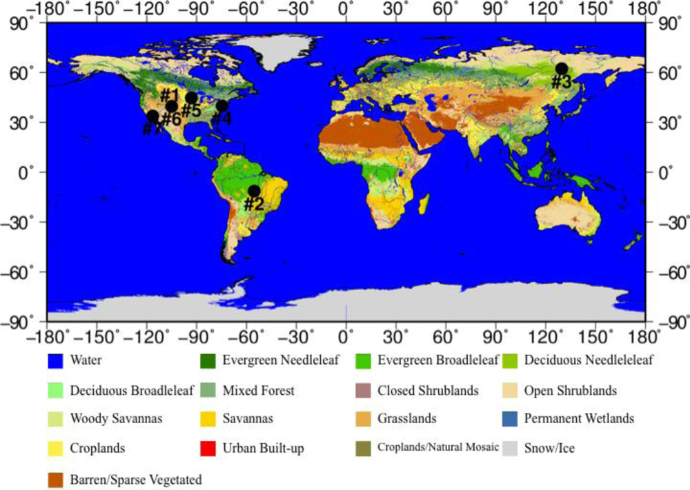
Figure 1. Normalized spectral response functions of select Advanced Spaceborne Thermal Emission and Reflection Radometer (ASTER) and Moderate Resolution Imaging Spectroradiometer (MODIS) bands. The sample reflectance spectra of vegetation and soils in the figure are obtained from the ASTER spectral library [20].
Remotesensing 04 02277f1
Figure 2. FLUXNET sites used in ASTER and MODIS Enhanced Vegetation Index (EVI) compatibility analysis mapped on MODIS 2007 International Geosphere-Biosphere Programme (IGBP) land cover data (MCD12Q1, Collection 5). The numbers in this figure correspond to those in Table 1.
Remotesensing 04 02277f2
Figure 3. Example of MODIS (a) and ASTER (b) pixel extractions. This area is classified as Deciduous Needle-leaf forest (Yakutsk, Russia) on MODIS 2007 IGBP. Each red box in (b) corresponds to a 3 km-by-3 km extraction area, that is, a 201-by-201 pixel area on ASTER and a 6-by-6 pixel area on MODIS.
Remotesensing 04 02277f3
Figure 4. Scatterplots of MODIS vs. ASTER VIs with ASTER reflectances aggregated without MODIS PSF. (a) ASTER Normalized Difference Vegetation Index (NDVI) vs. MODIS NDVI, (b) ASTER EVIB vs. MODIS EVI, (c) ASTER EVIP vs. MODIS EVI, (d) ASTER EVIC vs. MODIS EVI, (e) DNDVI vs. MODIS NDVI, (f) DEVIB vs. MODIS EVI, (g) DEVIP vs. MODIS EVI, (h) DEVIC vs. MODIS EVI, (i) RDNDVI vs. MODIS NDVI, (j) RDEVIB vs. MODIS EVI, (k) RDEVIP vs. MODIS EVI, (l) RDEVIC vs. MODIS EVI.
Remotesensing 04 02277f4
Figure 5. Same as Figure 4, but with ASTER reflectances aggregated with MODIS PSF. (a) ASTER NDVI vs. MODIS NDVI, (b) ASTER EVIB vs. MODIS EVI, (c) ASTER EVIP vs. MODIS EVI, (d) ASTER EVIC vs. MODIS EVI, (e) DNDVI vs. MODIS NDVI, (f) DEVIB vs. MODIS EVI, (g) DEVIP vs. MODIS EVI, (h) DEVIC vs. MODIS EVI, (i) RDNDVI vs. MODIS NDVI, (j) RDEVIB vs. MODIS EVI, (k) RDEVIP vs. MODIS EVI, (l) RDEVIC vs. MODIS EVI.
Remotesensing 04 02277f5
Figure 6. Scatterplots of ASTER NDVI and EVI aggregated with vs. without MODIS square point spread function (PSF). (a) ASTER NDVI by aggregation method without MODIS PSF vs. aggregation with MODIS PSF, (b) EVIB without MODIS PSF vs. aggregation with MODIS PSF, (c) EVIP without MODIS PSF vs. aggregation with MODIS PSF, (d) EVIC without MODIS PSF vs. aggregation with MODIS PSF, (e) ASTER NDVI without MODIS PSF vs. DNDVI, (f) ASTER EVIB without MODIS PSF vs. DEVIB, (g) ASTER EVIP without MODIS PSF vs. DEVIP, (h) ASTER EVIC without MODIS PSF vs. DEVIC, (i) ASTER NDVI without MODIS PSF vs. RDNDVI, (j) ASTER EVIB without MODIS PSF vs. RDEVIB, (k) ASTER EVIP without MODIS PSF vs. RDEVIP, (l) ASTER EVIC without MODIS PSF vs. RDEVIC.
Remotesensing 04 02277f6
Table 1. FLUXNET sites used in ASTER and MODIS EVI compatibility analysis.
No.Site NameLongitude, Latitude [Decimal Degrees]Land Cover Type 1Image Acquisition Date
1Niwot Ridge, CO, USAN40.033, W105.546Evergreen Needle-leaf forest2007.08.08
2Sinop-Mato Grosso, BrazilS11.412, W55.325Evergreen Broad-leaf forest2008.07.26
3Yakutsk, RussiaN62.241, E129.651Deciduous Needle-leaf forest2008.06.02
4Silas Little Experimental Forest, NJ, USAN39.914, W74.596Deciduous Broad-leaf forest2007.06.09
5Rosemount, MN, USAN44.722, W93.089Croplands2007.06.20
6South Denver, CO, USAN39.659, W105.013Urban and built-up2007.09.25
7Sonoran Desert, CA, USAN33.817, W116.373Barren or sparsely vegetated2007.09.12
1These land cover types were obtained from the 2007 International Geosphere-Biosphere Programme (IGBP) land cover type information from the MODIS standard, 1 km yearly land cover product (MCD12Q1, Collection 5).
Table 2. RMSE of ASTER NDVI/EVIs against MODIS NDVI/EVI.
NDVIEVIBEVIPEVIC
Aggregated without MODIS PSF0.0460.0180.0180.018
Aggregated with MODIS PSF0.0460.0190.0190.019
Table 3. Average of MODIS and ASTER reflectances with or without MODIS PSF for each band and each land cover type.
MODIS BlueMODIS RedMODIS NIRASTER Red without MODIS PSFASTER Red with MODIS PSFASTER NIR without MODIS PSFASTER NIR with MODIS PSF
Deciduous Broad-leaf0.0220.0270.4670.0370.0370.4520.449
Open Shrubland0.0750.1550.2090.1800.1770.2260.222
Deciduous Needle-leaf0.0320.0370.2350.0500.0500.2330.231
Evergreen Needle-leaf0.0060.0330.1610.0610.0600.1760.175
Evergreen Broad-leaf0.0160.0230.2870.0340.0340.2610.260

