Global Navigation Satellite Systems Reflectometry as a Remote Sensing Tool for Agriculture

Abstract

The use of Global Navigation Satellite Systems (GNSS) signals for remote sensing applications, generally referred to as GNSS-Reflectometry (GNSS-R), is gaining increasing interest among the scientific community as a remote sensing tool for land applications. This paper describes a long term experimental campaign in which an extensive dataset of GNSS-R polarimetric measurements was acquired over a crop field from a ground-based stationary platform. Ground truth ancillary data were also continuously recorded during the whole experimental campaign. The duration of the campaign allowed to cover a full crop growing season, and as a consequence of seasonal rains on the experimental area, data could be recorded over a wide variety of soil conditions. This enabled a study on the effects of different land bio-geophysical parameters on GNSS scattered signals. It is shown that significant power variations in the measured GNSS reflected signals can be detected for different soil moisture and vegetation development conditions. In this work we also propose a technique based on the combination of the reflected signal’s polarizations in order to improve the integrity of the observables with respect to nuisance parameters such as soil roughness.

1. Introduction

Several active and passive remote sensing techniques, such as monostatic radars and microwave radiometers, have been proposed to measure key land parameters like soil moisture and vegetation biomass over wide areas. As it is well known, soil moisture is a key parameter in the surface hydrological cycle, which is essential for the understanding of the interaction between land surfaces and the atmosphere. Vegetation biomass plays a crucial role in the carbon cycle through the processes of carbon uptake and respiration. It is therefore a variable of paramount importance for global climate modeling and greenhouse emission inventories.

Despite the recognized importance of these parameters, providing the resolution and precision required by most climatological model remains a challenge. Global Navigation Satellite System Reflectometry (GNSS-R) could potentially overcome these limitations, since the use of GNSS signals as sources of opportunity would allow for very dense multistatic radar measurements at L-Band. Such measurements have been previously shown—both theoretically and experimentally—to be sensitive to soil moisture and vegetation parameters [1–9]. Nevertheless, in order to obtain precise soil moisture and vegetation biomass estimates, several aspects still need to be studied in depth.

The LEiMON project (Land Monitoring with Navigation Signals) is an activity promoted and funded by the European Space Agency (ESA) to gain a deeper understanding on the mechanisms regulating the interaction between land surface parameters such as soil moisture content (SMC), soil surface roughness and vegetation biomass, and the scattered GNSS signal characteristics. The work presented in this paper is the result of a combined effort of several partners: Starlab Barcelona (Spain); the Institute of Applied Physics-National Research Council (IFAC-CNR, Italy); and the Centre for Microwave remote sensing (CETEM, Italy).

In the following section, the basis for obtaining of soil reflectivity estimates with GNSS-R are shown. The third section describes the LEiMON long term experimental campaign, during which continuous polarimetric measurements of GNSS scattered signals and ground-truth data were recorded. The fourth section deals with the data analysis and discusses the effects of land bio-geophysical parameters on GNSS-R signals. Finally, conclusions and recommendations are provided in the fifth section.

2. Soil Reflectivity Measurements with GNSS-R Signals

Remote sensing of soil bio-geophysical parameters with GNSS-R relies on the variability of the soil dielectric properties associated to soil moisture and vegetation. This turns into changes of the effective soil reflectivity that can be measured by comparing the received power of the direct and reflected GNSS signals. Following the formulation proposed in previous works, such as [10,11], for a given time t, the signal from a transmitting GNSS satellite located at R⃗_t observed by a receiver at R⃗_r can be expressed as

$$u_d({\overrightarrow{R}}_r,t)=\sqrt{\frac{P_t{G}_t}{4\pi }}\sqrt{\frac{G_r{\lambda }^2}{4\pi }}a\left(t-\frac{R_d}{c}\right)\frac{e^{-jk{R}_d}}{R_d}{e}^{-j2\pi (f_c+f_D)t}$$

(1)

where P_t and G_t stand for the transmitted power and GNSS satellite antenna gain, respectively; G_r is the receiver antenna gain in the direction of the transmitting satellite; a(t) represents the modulating PRN code; f_c is the GNSS carrier frequency; k is the associated wavenumber (2π/λ); f_D is the Doppler frequency shift originated due to the relative velocity of transmitter and receiver; and R_d is the distance between transmitter and receiver, defined as |R⃗_t − R⃗_r|. The previous equation can also be used to express the field reflected from a perfectly flat surface; in such a case it can be considered that the actual source can be replaced by a mirrored one below the surface, assuming it as a punctual source at a distance R_0,sp + R_sp

$$u_{r,\text{sp}}({\overrightarrow{R}}_r,t)=\sqrt{\frac{P_t{G}_t}{4\pi }}\sqrt{\frac{G_r{\lambda }^2}{4\pi }}{ℛ}_{\text{sp}}a\left(t-\frac{R_{0,\text{sp}}+R_{\text{sp}}}{c}\right)\frac{e^{-jk(R_{0,\text{sp}}+R_{\text{sp}})}}{R_{0,\text{sp}}+R_{\text{sp}}}{e}^{-j2\pi (f_c+f_{D,\text{sp}})t}$$

(2)

where R_0,sp and R_sp are the distances from transmitter and receiver to the specular point, and $ℛ$_sp is the Fresnel reflection coefficient at the specular point.

For a rough surface, under the Kirchoff Approximation the reflected field can be expressed more generally as the superposition of all scattered fields from each single point on the surface. The final scattered field as observed by the receiver yields

$$u_r({\overrightarrow{R}}_r,t)=\frac{i\sqrt{P_t{G}_t}}{4\pi }\underset{s}{\int }\sqrt{\frac{G_r(\overrightarrow{\rho }){\lambda }^2}{4\pi }}ℛ(\overrightarrow{\rho })a\left(t-\frac{R_0(\overrightarrow{\rho })+R(\overrightarrow{\rho })}{c}\right)\frac{e^{-jk(R_0(\overrightarrow{\rho })+R(\overrightarrow{\rho }))}}{R_0(\overrightarrow{\rho })R(\overrightarrow{\rho })}{e}^{-i2\pi (f_c+f_D(\overrightarrow{\rho }))t}(\overrightarrow{q}\cdot \widehat{N})d\overrightarrow{\rho }$$

(3)

where G_r is the receiver antenna gain. P_t and G_t can be considered constant for all the scattering surface. q⃗ is the scattering vector defined as q⃗ = k(m̂ − n̂), where k is the wavenumber, N̂ is the vector normal to the local tangent plane, and q⃗ corresponds to the bisecting vector of the incident and scattered fields defining the plane that would specularly reflect the incident wave in the direction of the receiver.

Comparing Equations (1) and (2), it can be readily seen that in the case of low altitude receivers, soil reflectivity estimates could be obtained from the ratio of the reflected and direct fields, u_r,sp and u_d. However, the final scattered field is a combination of the coherent and incoherent scattering components, represented by Equations (2) and (3), respectively. The former is generated in the specular scattering direction and has a constant value driven by the Fresnel reflection coefficients. The latter has an omnidirectional nature and its amplitude has a random behavior that can be described by a two dimensional Gaussian distribution. For moderately rough surfaces (as it is the case for most terrain surfaces at L-band), a temporal averaging can be applied to the received signals as a means to mitigate the uncertainty of the incoherent component. Due to the ground-based configuration of the LEiMON experiment, a long coherent averaging could be performed for this purpose. Nonetheless, as will shown in Section 4, in some cases the incoherent scattering component could not be completely removed, leading to artifacts in the data.

In order to detect GNSS signals, the direct and reflected fields need to be cross-correlated with the PRN code replica for a given delay offset, τ, and a frequency shift with respect to the carrier, f. The correlation can be expressed as

$$Y(\tau ,f)=\frac{1}{T_i}{\int }_{T_i}{u}_{d,r}a(t-\tau ){\text{e}}^{i(f_c+f)t}dt$$

(4)

with T_i being the coherent integration time. For the direct signal, when the correlation is maximum, the PRN codes of both incoming signal and replica are aligned, i.e., τ corresponds to the signal propagation delay from transmitter to receiver, and f matches the Doppler shift due to the relative velocity between the GNSS satellite and receiver.

The estimated co- and cross-polarization reflection coefficients, Γ_LR and Γ_RR, can be defined as the ratio of the direct and reflected waveforms measured at different polarizations, $Y_{L,R}^{d,r}(\tau ,f)$, where L and R stand for left and right hand circular polarizations, respectively. For ground based receivers, the direct and reflected Doppler frequency shifts can be considered to be the same, thus the dependency with f can be dropped out for the sake of clarity. Applying the variable change τ′ = τ − R_d, it can be written that:

$$\begin{array}{l}{\mathrm{\Gamma }}_{LR}=\frac{{\left|\langle Y_L^r(\mathrm{\Delta }\tau )\rangle \right|}^2}{{\left|\langle Y_R^d(0)\rangle \right|}^2}\\ {\mathrm{\Gamma }}_{RR}=\frac{{\left|\langle Y_R^r(\mathrm{\Delta }\tau )\rangle \right|}^2}{{\left|\langle Y_R^d(0)\rangle \right|}^2}\end{array}$$

(5)

where 〈·〉 denotes the averaging operator along time. Δτ is the delay difference between the direct and reflected paths. In the case of ground-based or low altitude receivers this could be calculated with the simple equation c Δτ =2 h cos θ, with θ being the incidence angle. By selecting τ′=0 and τ′=Δτ for the direct and reflected waveforms, respectively, it is ensured that the waveforms’ peaks are selected.

3. LEiMON Experimental Campaign

The LEiMON Experimental Campaign was carried out on an agricultural area near Florence, along the Pesa River, Italy (43.673^°N, 11.128^°E), from March to September 2009. In this time period, an entire crop growing season was covered, and due to the seasonal rains, a high variability of soil moisture content was observed. In order to obtain different soil roughness conditions, the field was worked in different ways over the campaign. Throughout the experimental campaign, both GNSS-R data and ancillary data were continuously acquired. The next subsections describe the GNSS-R instrument used and the experimental campaign execution.

3.1. The GNSS-R Instrument

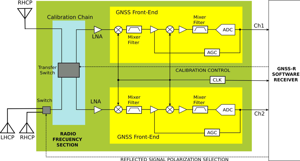
The GNSS-R instrument used for the LEiMON experimental campaign was designed and developed at Starlab Barcelona during the ESA project SAM (An Innovative Microwave System for Soil Moisture Monitoring), and upgraded during the LEiMON project. The final block diagram of the instrument can be seen in Figure 1.

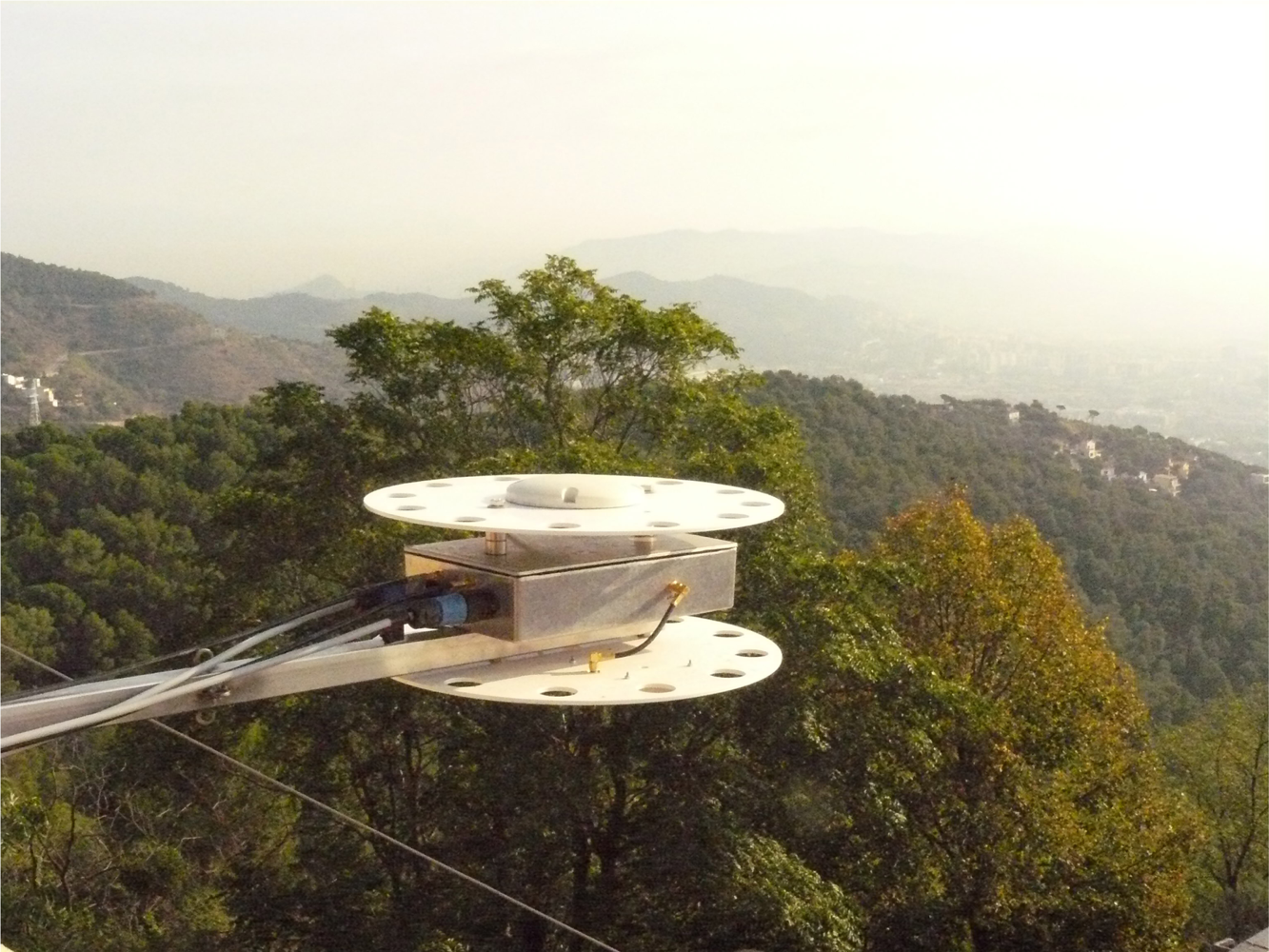
The SAM instrument features an up-looking GPS L1 right hand circular polarized (RHCP) antenna for the reception of the direct signal, and two down-looking antennas: a left hand circular polarized (LHCP) and a RHCP. The antenna rig of the GNSS-R instrument is shown in Figure 2. Both down-looking antennas share a common receiving channel and the operative antenna is selected at each time by a radio-frequency switch. A calibration chain was introduced for relative calibration of the two receiving channels. The GPS signals are digitized by off-the-shelf GNSS front ends, which work together using a common reference clock. The bitstreams are then transmitted to a software receiver that acquires and tracks the signals from the different GNSS satellites in view, and records the direct and reflected complex waveforms. In a final stage the time series of the waveforms peaks are extracted, and the reflectivity components Γ_LR and Γ_RR are calculated.

3.2. Experimental Campaign Execution

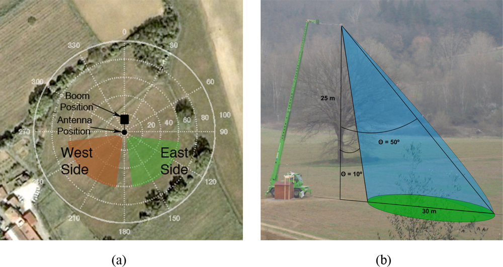
The GNSS-R instrument was installed in the center of a crop field on a hydraulic boom at a height of 25 m. An aerial view of the experimental test site is shown in Figure 3(a). The boom and antenna positions are depicted in the image. In order to procure the highest possible variability of soil conditions during the campaign, the experimental field was split up along a north-south line from the position of the receiver, dividing the experimental field in two halves, as shown in the figure. These will be referred from now on as the East and West field. These two sides of the field were worked in different ways, and had different soil conditions depending on the period of the campaign. The works performed on each of the fields are described in

Table 1. Summary of the most important field works performed during the experimental campaign.

Date	Works on East Field	Works on West Field
24–27 March	Plowed	Plowed
28 March	Harrowed	Rolled
3 May	Plowed	Plowed
5 May	Sorghum seeding	Plowed
10 May	-	Sunflower seeding
19 June	Sorghum re-seeding	-
4 August	Sorghum cut	-
23 August	Sorghum cut	Sunflower harvesting

.

The field works started towards the end of March. First, both fields were prepared with a general plowing. After that, the East field was harrowed, while the West field was rolled, obtaining two different soil roughness conditions: the East field was rougher, with a surface height standard deviation (σ_z) of 3 cm, whereas for the West field it was 1.8 cm. On early May, both fields were plowed again in order to prepare them for seeding. Sorghum and sunflower were the two selected crops for assessing the effect of different types of vegetation on GNSS-R signals. The former was seeded on the East field, and the latter on the West field. Unfortunately, due to adverse weather conditions, the sorghum did not sprout. A second seeding was carried out in mid-June. Despite this additional effort, due to the very late seeding the sorghum did not sprout. On the contrary, the sunflower grew up to 1.5 m and reached a plant water content of 7 kg/m² on its maximum development stage. On 23 August, the sunflower was harvested and the biomass was removed from the field. The campaign lasted until mid-September, during which time both fields remained bare.

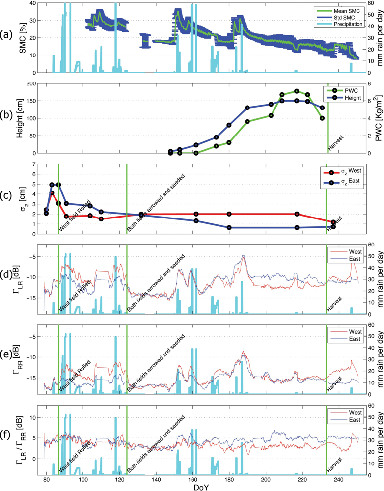
The ground truth and ancillary data comprised continuous soil moisture measurements, surface roughness, plant development parameters. In addition, a meteorological station was installed on the site in order to record several meteorological parameters such as daily rain, external air temperature, humidity, wind speed and air pressure. Soil moisture measurements of the first 10 cm of soil were continuously registered by six frequency domain reflectometry (FDR) probes DELTA-T SM 200 installed on the field and uniformly distributed over the field. These probes measure the volumetric soil moisture by responding to changes in the apparent dielectric constant of moist soil. A hand-held time domain reflectometry (TDR) probe IMKO TRIME DataPilot and soil gravimetric measurements were used to calibrate the FDR probes. As no significant differences were observed between the probes in the East and West sides, the calibrated FDR probe signals were averaged together in order to obtain a general SMC value for the whole experimental site. The averaged SMC for the whole experimental campaign and its associated standard deviation are represented together with the daily precipitation in Figure 4(a). Vegetation parameters such as plant density, leaf and stalk dimensions, number of leaves per plant, plant water content and moisture were measured periodically on a weekly basis following standard measuring procedures as described in [12]. The sunflower height and plant water content are shown in Figure 4(b). Surface roughness was measured using a 2 m long needle profilometer with a sampling interval of 0.8 cm. Three contiguous profiles were acquired for each measurement in order to diminish the effect of possible irregularities in the terrain in the reconstruction of the surface roughness profile. The achieved profiles were then digitized and re-sampled at a constant interval in order to calculate the height standard deviation σ_z, and the correlation length l_c. The East and West surface roughness for the whole campaign are depicted in Figure 4(c).

4. Data Analysis

Two types of data analysis were performed on the GNSS-R data. In the first one, the temporal evolution of the GNSS-R signals were compared to the ground-truth data. The second analysis deals with the spatial distribution of GNSS-R signals and their dependency with incidence angle, together with a quantitative determination of the GNSS-R signals’ sensitivity to soil moisture and vegetation.

4.1. GNSS Reflected Signals Active Scattering Areas

As mentioned in the previous section, the experimental test site was divided in two halves: the East and West fields. The GPS satellites’ azimuth angle was used to assign the reflectivity measurements obtained for each individual satellite to its corresponding side of the field. Thus, satellites with an azimuth angle between 100^° and 270^° were assigned to the East field, and satellites with azimuth between 190^° and 260^° to the West field, as depicted in Figure 3(a). A 20^° azimuth gap was allowed between both field sides to avoid mixed-pixel effects on the reflected signals. In addition, only reflectivity measurements obtained from satellites with an incidence angle between 10^° and 50^° were considered in order to avoid undesired reflections. The lower limit is set so that multipath signals from the boom structure could be avoided, whereas the upper limit corresponds to the beam-width of the receiving antenna. In Figure 3(b) a sketch is provided in order to illustrate this situation.

4.2. GNSS-R Signal Temporal Data Analysis

For the temporal analysis, the GPS satellites in view during each data take were averaged together in order to obtain the time series of the Γ_LR and Γ_RR reflectivity coefficients. Despite the fact that the reflectivity coefficients change with incidence angle, this analysis was carried out in order to identify temporal trends on the data, and to establish qualitative relationship among the geo-physical parameters and the GNSS-R signals. A one-day moving average was applied to the time series in order to reduce the intrinsic measurement noise.

Figure 4(d–f) displays the time series for the measured reflectivity coefficients Γ_LR, Γ_RR, and the ratio of both, respectively. Superimposed on the graphs, the daily accumulation of rain (in mm) and the most significant field works have also been represented.

As can be seen from the plots, Γ_LR and Γ_RR experience remarkable increases directly related to rain events, producing power variations of up to 7 dB in the Γ_LR coefficient. In addition, it can be observed that the obtained reflectivity coefficients follow the general trend of the SMC measured with the FDR probes, shown in Figure 4(a). Nonetheless, there are some discrepancies between the soil moisture probe data and the estimated reflectivity coefficients. A remarkable increase in the GNSS-R signals can be observed between DoY 170 and 175. This is related to light rain events that took place on those days. However, the average SMC measured by the probes does not experience a significant variation. The same situation is evidenced for a light rain event that occurred on DoY 217. These results were linked to the fact that GNSS-R signals are sensitive to the soil moisture in the first centimeters of soil, whereas the FDR probes obtain the soil moisture measurements at 10 cm from the surface, which might not suffer any variation in case of small rain events.

The effect of roughness is also clearly visible in the two reflection coefficients. In the beginning of the campaign, both reflectivity coefficients followed the same behavior, since the soil conditions were the same in both sides of the field. However, after the field works on 28 March, day of the year (DoY) 87, the East and West sides of the field had different soil roughness conditions: 3 cm in the case of the East field and 1.8 cm for the West field. As a result, a 3 dB difference between the West (smooth) and East (rough) fields could be observed in the Γ_LR and Γ_RR reflectivity coefficients. After the second plowing event, when both fields were prepared for seeding (3 to 5 May), DoY 123–125, the roughness of both fields was again homogenized, and therefore the difference in the power of the signals coming from both sides of the field disappeared.

In the beginning of June, DoY 150, the difference between the East and West sides started to increase for Γ_LR, reaching its maximum by late July, DoY 210. This observation was linked to the attenuation introduced by the developing sunflowers on the West field, Figure 4(b), while the East field remained bare or scarcely vegetated. After the harvest, around 20 August, DoY 232, this difference is reduced.

In the case of the RHCP signal, no significant difference between the bare and vegetated sides of the field could be observed. A possible explanation for this is that volume scattering was produced by the sunflower canopy as the GNSS signals traversed the vegetation layer. This incoherent scattering component would compensate for the signal attenuation produced by vegetation. After harvest, an important increase on the Γ_RR component on the west side was observed. This effect could be linked to the removal of biomass from the field, thus eliminating the attenuation produced by vegetation. However, vertical sunflower stalks were left on the West field, which could still depolarize the impinging signal by a volume scattering effect. The combination of these two effects could have led to the increase in the Γ_RR component.

Regarding the ratio of the two reflectivity components, it can be observed that it is moderately sensitive to rain events, with about 3 dB difference between wet and dry soil moisture conditions. A remarkable aspect is that, unlike Γ_LR and Γ_RR, variations in roughness conditions are not detected by this observable, as can be seen in Figure 4(f); despite the soil roughness difference between the East and West field between late March and early May, DoY 87–123, the Γ_LR over Γ_RR ratio does not present any appreciable difference, which could make this observable suitable for roughness-independent soil moisture remote sensing. This result confirms the hypothesis initially proposed in [13], where it is shown that for moderately rough surfaces the ratio of two orthogonal polarizations does not depend on the surface roughness.

4.3. Sensitivity Determination of GNSS-R Signals to Soil Bio-Geophysical Parameters

In order to assess the sensitivity of GNSS-R signals to soil parameters, four different periods of the campaign were selected for their stable conditions and high diversity of bio-geophysical parameters.

Table 2. Selected time periods for the estimation of the sensitivity of GNSS-R signals to land bio-geophysical parameters.

Period	Dates	DoY	SMC	Roughness	Vegetation
1	8–10 April	98–100	30%	East σz =3.0 cm, West σz =2.0 cm	East bare, West bare
2	20–23 May	140–143	17%	East σz =2.0 cm, West σz =2.0 cm	East bare, West bare
3	28–30 June	179–181	17%	East σz =0.7 cm, West σz =2.0 cm	East bare, West SF (45 cm)
4	18–20 July	199–201	20%	East σz =0.7 cm, West σz =2.0 cm	East bare, West SF (135 cm)

summarizes the most relevant soil conditions for these periods.

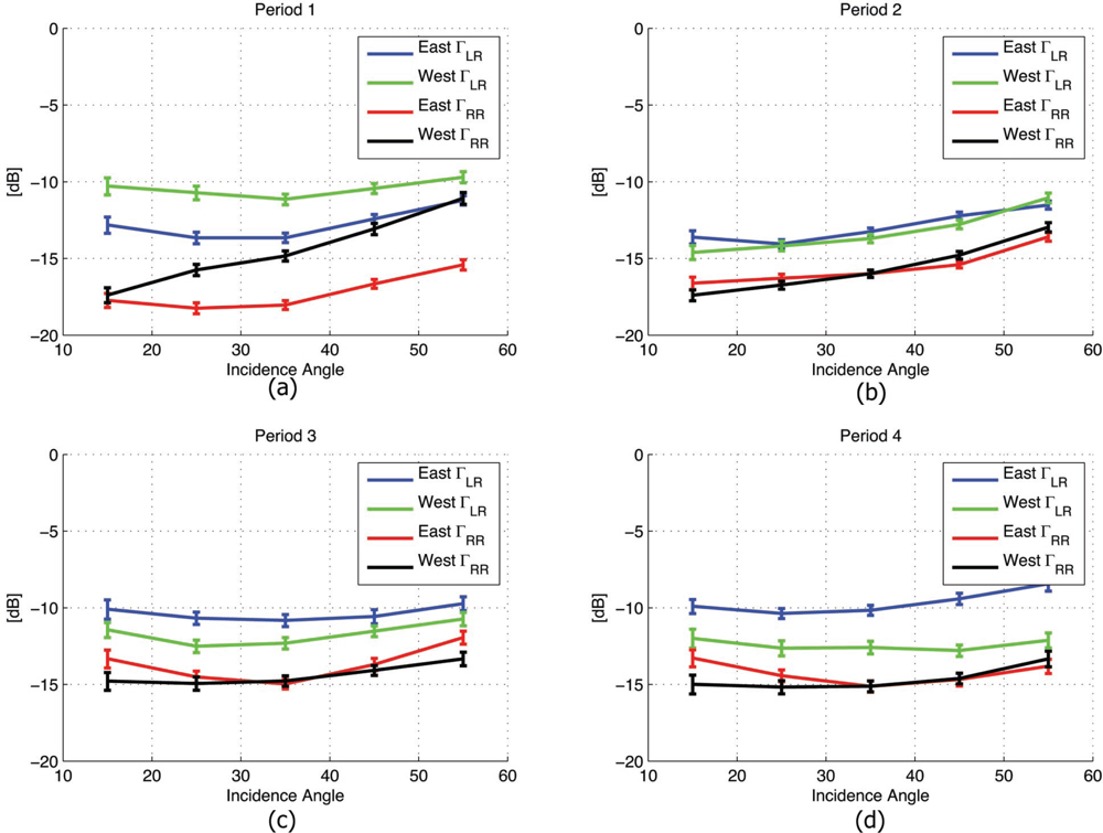
As in the temporal data analysis, the signals were separated among the East and West fields. The dependency with the incidence angle was also considered in order to compare the data with the scattering models. Figure 5 provides the mean values of the measured Γ_LR and Γ_RR for both fields and their associated measurement uncertainty. From this figure, the effect on the GNSS-R signals of soil surface roughness, SMC, and vegetation PWC can be determined. For soil roughness, in Period 1 (Figure 5(a)), signals coming from the East field are lower than those of the West field by an average of 2.3 dB due to the difference in surface height standard deviation. Regarding SMC, on Period 1 (wet, SMC = 30%) and on Period 2 (dry, SMC = 17%) for the West field (similar soil roughness conditions) Γ_LR presents a difference of 3.5 dB between wet and dry soil moisture conditions. Finally, for vegetation PWC observing the bottom panels on Figure 5, corresponding to Periods 3 and 4, an increasing difference in Γ_LR between the East (bare) and the West field (vegetated) can be observed. This difference reaches 2 dB when vegetation approaches its maximum development stage in Period 4 due to the attenuation effect of the vegetation layer.

In order to determine quantitative indicators (sensitivity and correlation coefficient) of the relation between GNSS-R signals and land bio-geophysical parameters, the averaged values calculated for Γ_LR, Γ_RR and the ratio of both were compared to the soil moisture FDR probes mean values and to the in situ plant-related measurements. This sensitivity analysis was done over a dataset of 25 periods of 3 days, each distributed over the whole duration of the campaign in which the land conditions were considered stable. For the analysis of soil moisture sensitivity, the selected period was from early April to early June (DoY 90–150). During this period a complete soil moisture cycle is covered and very stable surface roughness conditions are ensured in the West field. On the East field the soil roughness variation is high and therefore the coupled effect on the signal of SMC and roughness is observed. For the analysis of the vegetation development, the PWC was considered, as it is the main parameter representing the biomass. For this analysis the period corresponding to the whole sunflower’s development cycle was selected, i.e., between mid-June and early August (DoY 165–210). Similar to the temporal signal analysis, the GNSS-R data were separated among the East and West fields and averaged over a range of incidence angles from 20^° to 40^°. This allows to reduce uncertainty in the measurements and it does not affect the final results, since, as can be observed in Figure 5, the reflectivity coefficients does not change remarkably in this incidence angle range.

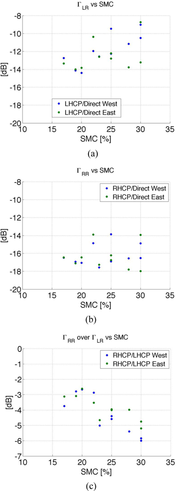
Figure 6 gathers the scatter plots of the measured reflection coefficients vs. SMC. The sensitivity of the measured reflection coefficients with respect to soil moisture was obtained by fitting a linear model to the data. For Γ_LR, Figure 6(a), the sensitivity was determined to be 0.3 dB/SMC(%) for the West field, with a Pearson correlation coefficient of 0.76. For the East field the sensitivity and correlation coefficient decrease due to changes in surface roughness conditions. For the Γ_RR coefficient, both sensitivity and correlation with respect to soil moisture are very low. However, it was found that the ratio Γ_RR over Γ_LR presents a high correlation coefficient with soil moisture content, 0.84, even for varying surface roughness. The sensitivity of both reflectivity coefficients ratio yields 0.2 dB/SMC(%). This fact alone demonstrates the value of GNSS-R polarimetric observations for land applications.

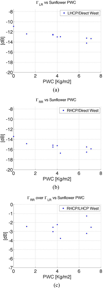
The results for the PWC sensitivity analysis are shown in Figure 7. The correlation coefficient for both Γ_LR and Γ_RR reflection coefficients yields 0.8. In this case the sensitivity for both polarizations equals 0.3 dB/(Kg/m²), which suggests an attenuation effect of the vegetation biomass to the GNSS reflected signals. Unlike for SMC, the ratio of the reflection coefficients for both polarizations does not present a clear correlation with the PWC.

4.4. GNSS-R Data Analysis Further Considerations

Apart from the effect of land bio-geophysical parameters on GNSS scattered signals, some other remarkable features can also be observed in the data. The first one is the increase of Γ_LR with incidence angle, although it is expected from Fresnel reflection theory that this parameter decreases to zero at grazing incidences. This effect is linked to a polarization mismatch between the incident wave and the GNSS receiving antenna [14,15], which was also observed during the SAM project. The reflection coefficients are given in an orthogonal plane to the direction of propagation of the reflected wave; however, this is not a general case, and therefore their effective polarization and reflectivity are modified by the projection of the polarization vector of the reflected wave to the antenna plane.

A second noticeable aspect is the difference between the Γ_RR and the Γ_LR reflection coefficients. While theoretical models predict a difference between 10 and 20 dB, in some particular situations, the maximum difference measured for the reflection coefficients was around 7 dB. The cause of that was linked to three possible aspects. Firstly, the limited sensitivity of the receiver, which is estimated to be around a reflectivity value of −20 dB, could have prevented the acquisition of the entire dynamic range of the RHCP reflected signal, thus introducing a bias on the measured RR coefficient. Secondly, note the limited cross-polarization isolation of the receiving antennas. The GPS antennas used in the campaign were characterized in an anechoic chamber, and the cross-polarization isolation at boresight was determined to be −17 dB for both LHCP and RHCP down-looking antennas. This has an influence in the determination of the absolute value of Γ_RR, but it is not expected to affect the general conclusions of this work. And thirdly, note the aforementioned ellipticity of the impinging GNSS signals. As stated in the GPS Interface Specifications Document (ICD-200-D), the ellipticity of GPS incident waves should not exceed 1.2 dB in the whole field of view of the GPS satellites. However, this is a non-negligible ellipticity factor that should be measured and accounted for in order to perform precise GNSS-R polarimetric measurements.

5. Conclusions and Future Work

The work presented in this paper demonstrates the capabilities of GNSS-R polarimetric observations as a remote sensing tool for agricultural applications from ground-based receivers. The extensive dataset, gathered during an on-ground experimental campaign conducted for 6 months on an agricultural field, allowed to compare the recorded GNSS-R signals with bio-geophysical processes, and to determine the effect of surface roughness, soil moisture content (SMC), and plant water content (PWC) on the GNSS-R reflected signals.

Significant power variations in the measured reflection coefficients could be detected for different soil moisture and vegetation development stages. For stable soil roughness conditions, the estimated left-right reflection coefficient, Γ_LR, presents a sensitivity to soil moisture of 0.3 dB/SMC(%) with a correlation coefficient of 0.76, whereas the right-right reflection coefficient, Γ_RR, has very low sensitivity and correlation values. Changes in the soil roughness severely affect the reflected GNSS signal power, decorrelating Γ_LR from soil moisture observations. In spite of this, it was demonstrated that the ratio between both reflection coefficients is scarcely affected by soil roughness variations; with a sensitivity of 0.2 dB/SMC(%) and a correlation coefficient of 0.84 with respect to SMC, this parameter could therefore represent an optimum observable for soil moisture remote sensing. Regarding the sensitivity to vegetation characteristics, it was observed that Γ_LR and Γ_RR present a significant response to PWC (correlation coefficient 0.8, sensitivity 0.3 dB/(Kg/m²)). The ratio of both reflection coefficients is not sensitive to the presence of vegetation, indicating an attenuation effect of vegetation on the GNSS reflected signal.

The authors have identified that in order to be able to perform precise GNSS-R polarimetric measurements, some other relevant aspects should be addressed. Firstly, the receiver’s sensitivity as well as the cross-polarization isolation characteristics of the receiving antennas should be improved in order to allow to measure the whole dynamic range of the Γ_RR reflection coefficient. Secondly, an additional radio-frequency channel should be introduced to measure the direct LHCP polarization, and therefore achieve a better knowledge of the polarization ellipticity of incident GNSS signals.

Future work will concentrate on the upgrade of the GNSS-R instrument according to these recommendations, the development of algorithms for simultaneous soil moisture content and vegetation PWC retrieval, and the assessment of the potentialities of this technology for soil moisture and vegetation biomass monitoring from space-borne platforms employing the simulator developed during the LEiMON project.