Overcoming Limitations with Landsat Imagery for Mapping of Peat Swamp Forests in Sundaland
by
 ,
,
Lahiru S. Wijedasa
1,2,3,*, 
Sean Sloan
4,
Dimitrios G. Michelakis
5 and
Gopalasamy R. Clements
3,4,6 1
Singapore Botanic Gardens, 1, Cluny Road, Singapore 259569, Singapore
2
Royal Botanic Garden Edinburgh, 20a Inverleith Row, Edinburgh EH3 5LR, UK
3
Rimba, 18E Kampung Basung, Kuala Berang 21700, Terengganu, Malaysia
4
Centre for Tropical Environmental and Sustainability Science and School of Marine and Tropical Biology, James Cook University, Cairns, QLD 4870, Australia
5
School of Geosciences, University of Edinburgh, Geography Building, Drummond Street, Edinburgh EH8 9XP, UK
6
Center for Malaysian Indigenous Studies, University Malaya, 50603 Kuala Lumpur, Malaysia
*
Author to whom correspondence should be addressed.
Remote Sens. 2012, 4(9), 2595-2618; https://doi.org/10.3390/rs4092595
Submission received: 11 July 2012
/
Revised: 3 September 2012
/
Accepted: 4 September 2012
/
Published: 10 September 2012
(This article belongs to the Special Issue Remote Sensing of Biological Diversity)
Abstract
:Landsat can be used to map tropical forest cover at 15–60 m resolution, which is helpful for detecting small but important perturbations in increasingly fragmented forests. However, among the remaining Landsat satellites, Landsat-5 no longer has global coverage and, since 2003, a mechanical fault in the Scan-Line Corrector (SLC-Off) of the Landsat-7 satellite resulted in a 22–25% data loss in each image. Such issues challenge the use of Landsat for wall-to-wall mapping of tropical forests, and encourage the use of alternative, spatially coarser imagery such as MODIS. Here, we describe and test an alternative method of post-classification compositing of Landsat images for mapping over 20.5 million hectares of peat swamp forest in the biodiversity hotspot of Sundaland. In order to reduce missing data to levels comparable to those prior to the SLC-Off error, we found that, for a combination of Landsat-5 images and SLC-off Landsat-7 images used to create a 2005 composite, 86% of the 58 scenes required one or two images, while 14% required three or more images. For a 2010 composite made using only SLC-Off Landsat-7 images, 64% of the scenes required one or two images and 36% required four or more images. Missing-data levels due to cloud cover and shadows in the pre SLC-Off composites (7.8% and 10.3% for 1990 and 2000 enhanced GeoCover mosaics) are comparable to the post SLC-Off composites (8.2% and 8.3% in the 2005 and 2010 composites). The area-weighted producer’s accuracy for our 2000, 2005 and 2010 composites were 77%, 85% and 86% respectively. Overall, these results show that missing-data levels, classification accuracy, and geographic coverage of Landsat composites are comparable across a 20-year period despite the SLC-Off error since 2003. Correspondingly, Landsat still provides an appreciable utility for monitoring tropical forests, particularly in Sundaland’s rapidly disappearing peat swamp forests.
1. Introduction
Peat swamp forests are of tremendous conservation importance because of their high levels of species endemism [1], as well as their ability to store huge volumes of carbon as organic peat below ground [2,3]. These ecosystems are disappearing rapidly due to forest conversion and fires, which have contributed significantly to global carbon emissions [4,5]. At current deforestation rates, peat swamp forests in Southeast Asia may disappear by 2030 [6]. Conservation planners urgently require reliable and up-to-date spatial baselines for such threatened ecosystems [7]. Satellite imagery arguably provides the best means to map and monitor large swathes of tropical forests [8]. Most remote sensing studies mapping peat swamp forests across Southeast Asia have favored the use of 250-m MODIS imagery [6,9–13]. However, we argue that, with proper treatment, finer-scale Landsat imagery can provide an alternative perspective on this highly fragmented forest type.
With global coverage, medium spatial resolution (30–80 m), and the largest historical archive of regularly-acquired, freely available space-based Earth observations [14], Landsat imagery has proven an invaluable resource for monitoring tropical forests [15–18]. Unfortunately, several issues with Landsat may discourage their use for contemporary tropical forest monitoring [14]. First, from the outset, Landsat has been blighted by persistent cloud cover at tropical latitudes [19], more so than other optical sensors because of its 16–18 day revisit period. In Central Sumatra, Nezry et al. [20] calculated the probability of acquiring either a Landsat MSS, Landsat TM or SPOT-HRV image with <70% cloud cover in a given year at only 26%. Second, the Landsat-5 satellite, one of two remaining in service, no longer has global coverage due to an insufficient number and distribution of ground receiving stations [14]. Third, the Landsat-7 satellite sensor suffered a hardware failure in its scan line corrector (SLC) in 2003, resulting in the loss of ∼22–25% data in each scene [21–23]. The missing areas due to the SLC-Off error appear as parallel stripes of no-data values on either side of an unaffected 22-km swath in the centre of the scene (Figure 1(a,b)), where the stripes range from one 30-m pixel near the scene centre to fourteen 30-m pixels (i.e., 420 m) near the scene edge (Figure 1(d)) [21,22,24].
Unsurprisingly, estimates of peat swamp forest extent and loss across Southeast Asia have favored the use of MODIS imagery [6,9–13], which has a faster revisit period (i.e., more cloud-free views), no missing-data issues, a wider field-of-view, but a more moderate spatial resolution (250 m) than Landsat. The role of Landsat imagery in such studies has largely been to calibrate and/or assess MODIS signals [6], or to yield spatially-coarsened pre-MODIS mosaics as referents for modern-day MODIS estimates [6,18,25]. It is highly plausible that the SLC-Off issue is a major factor in the decision to use MODIS rather than Landsat for large-area mapping.
Despite its limitations, Landsat imagery has attractive qualities in the context of monitoring regional changes to forest habitat and biodiversity [26–30]. Its relatively high spatial resolution discriminates intact, disturbed, and regenerating forests in heterogeneous landscapes more accurately than coarser imagery [18,31,32], and better detects smaller forest fragments as well as smaller-scale perturbations important for conservation planning (e.g., illegal roads, logging roads [32,33]). As such, given its long historical record (1970s–present, depending on location), Landsat is well-positioned to track changes to habitat quality at decadal intervals—an important point considering the accruement of ‘extinction momentum’ with declines in habitat integrity and connectivity [34]. Such qualities are particularly attractive for monitoring peat-forest loss in Sundaland. Therein, highly biodiverse peat swamp forests [1] have been reduced to less than half their original extent [6], and are increasingly being fragmented. In effect, peat swamp forest fragments are assuming higher conservation priority in proportion to their rapidly shrinking and fragmented distribution, and thus require spatial monitoring that is both geographically extensive and fine-grained.
Compositing of Landsat images provides a means of addressing data gaps related to sensor error (SLC-Off) and cloud cover [10,14,23,35,36]. By combining multiple images for each scene, areas missing in one image can be ‘filled’ with valid values of coincident images of a similar acquisition date. The exact position of the stripes of missing-data varies between Landsat images, ranging from no overlap to almost complete overlap in SLC-Off error (Figure 1). This variation in position also accounts for variation in the number of images needed to reduce missing data in each scene to generally acceptable levels. Figure 1 illustrates that, in the absence of cloud cover, 2 to 4 images per scene may be sufficient to reduce missing-data areas to nil. Further, while the SLC-Off missing-data areas are greatest at scene edges, there is also a 30-km wide swath at the edge that overlaps the adjacent scene (Figure 1(a,d)), allowing the missing data in the swath to be more easily reduced when compositing scenes into a regional mosaic. Wulder et al. [14,23] provide a synopsis of common compositing methods used for Landsat, which may entail complex spatio-statistical interpolations and normalizations to composite spectral values, yet they cannot overcome seasonal spectral discrepancies within a scene composed of images from different seasons. Where land-cover change is rapid—as it is in the case of peat swamp forest loss—there is also a risk that the spectral composite may inadvertently incorporate such changes [37]. Simpler approaches to compositing have a corresponding appeal.
Here, we describe and test a method of post-classification compositing of Landsat imagery to facilitate multi-decadal monitoring of peat swamp forest cover in Sundaland. Specifically, we classify, composite, and mosaic 238 Landsat images over 58 scenes for 2005 and 2010, and compare the classification accuracy and missing-data extent of these products to our classified 1990 and 2000 GeoCover products composited with an additional 22 and 18 Landsat images, respectively. We illustrate the effect of image compositing using three test scenes, and quantify the missing-data areas owing to SLC-Off and cloud cover separately in these scenes. Finally, we make comparisons between Landsat- and a MODIS-derived classification of peat swamp forest cover to illustrate differences having implications for biodiversity monitoring.
2. Study Area
The study area of Sundaland is defined as the original extent (i.e., prior to anthropogenic land-cover change) of peat swamp forest in Peninsular Malaysia, Sumatra, and Borneo. This extent spans some 20.3 million hectares and 58 Landsat scenes (Figure 2). The study area contains one of the world’s greatest concentrations of peat swamp forests, which in turn host high levels of biodiversity and endemism [1] and store huge volumes of below-ground carbon—55 Gt alone for Indonesia [2,3,5]. Since 1990 an accelerating ascent of oil-palm plantations has driven widespread conversion of peat swamp forests, particularly in Sumatra, where only 28% of original peat-forest cover remains [6].
3. Methods
Our methods are summarized as follows. First, to delimit the study area, a map of original peat swamp forest extent was made based on soil and vegetation maps. Second, 268 Landsat images and 24 tiles for the GeoCover products covering the study area in Sundaland were classified for four time stamps circa 1990, 2000, 2005 and 2010. Third, contemporaneous classified images were composited to yield regional peat swamp forest cover maps for each time stamp. Fourth, an independent reference dataset was compiled, and the accuracy and coverage of the regional composite mosaic maps were assessed against it. To study the effect of compositing on the reduction of missing-data areas due to cloud/shadow and the SLC-Off issue separately, the percent decline in missing-data area was measured for three scenes of the 2010 mosaic. These scenes were selected based on similar proportion of study area per scene and to be from the same general region of the study area. To compare the minimum patch size observed using our Landsat mosaics and a comparable MODIS mosaic, we extracted patches of primary peat swamp cover from our 2000 Landsat mosaic and the 2000 MODIS mosaic of Miettinen et al. [11] and compare their patch-size frequency distributions.
3.1. Original Peat Swamp Forest Cover Map
We define the study area as the original extent of peat swamp forest cover prior to anthropogenic land-use change. We estimated this area based on historical soil maps, vegetation maps, topographical data and satellite imagery. To account for peat swamp areas cleared prior to 1990, we initially defined the original extent of peat swamp forest as that of peat soil areas according to historical soil maps [38–43]. As peat swamp forests are by definition found on permanently-inundated soils of at least half a meter in depth and with a loss of mass on ignition greater than 65–75% [44–47], a soil class apparent in soil maps, our initial delimitation of original extent was plausible. As a soil map for Brunei was not available, we used a Brunei vegetation map [48] to approximate original peat swamp forest cover extent therein.
Despite the fact that permanently inundated peat soils of depths >0.5 m are only known to support peat swamp forest [45,47,49–52], our initial estimate alone may still overestimate original peat swamp forest extent. We therefore refined this initial estimate by excluding from it all non-peat-swamp-forest primary vegetation types (e.g., freshwater’ swamp, mangrove and dipterocarp forests) delimited in historic vegetation maps [48,49,53–55] or visually identified in Landsat TM false-color composites (RGB 247) of the 1990 Landsat GeoCover product [56]. It was noted that vegetation maps, particularly those created using a combination of aerial photographs and ground truthing, appeared to have a higher accuracy than the soil maps when compared with our visual interpretations of the 1990 GeoCover product. We therefore assumed that a primary non-peat swamp forest vegetation type located on peat soil according to the soil maps was most probably an error in the soil map. Finally, given the requirement of flat topography for peat swamp forest, we similarly excluded from the initial estimate all areas with relatively closely packed contour lines which were indicative of hilly terrain according to SRTM data [57]. The final estimated extent of original peat swamp forest is shown in Figure 2.
3.2. Satellite Imagery
In total, 268 Landsat images and 24 GeoCover tiles for circa 1990, 2000, 2005 and 2010 were downloaded, classified, and composited into regional mosaics spanning the 58 scenes of the study area. All images in the Landsat GeoCover dataset [56] from January 1985 till December 2010 were considered. We accepted all images having mostly cloud free views of peat swamp forest areas, regardless of the overall cloud cover of the image, which occasionally reached 90%. Figure 2a and 2b illustrates the number of images used per scene for the 2005 and 2010 composites.
At the time of analysis (December 2010), only a limited number of Landsat images for 1990 and 2000 were publicly available. Therefore, we used the 1990 and 2000 Landsat GeoCover products [56] (12 mosaicked tiles of multiple composited Landsat images) for these years. The documentation for these GeoCover mosaics did not specify the number of images composited per scene. We therefore estimate this by counting the images per scene used in the 2005 mosaic, for those scenes for which no SLC-Off images were included (n = 32 scenes). To these 1990 and 2000 mosaics we added 22 and 18 further images respectively to fill data gaps due to cloud and shadow. The range of image acquisition years in the final, composited mosaics are 1989–1991, 1999–2001, 2004–2006 and 2009–2010.
3.3. Image Classification
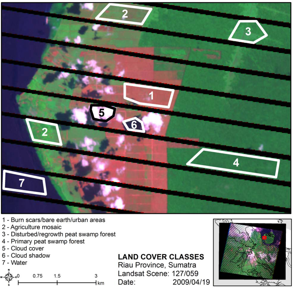
We adopted a maximum-likelihood supervised classification approach to classify individual, images into five land covers (Table 1 and Figure 3): primary peat swamp forest, disturbed/re-growth peat swamp forests, agriculture mosaic, bare earth/urban areas/burn scars, and missing data (includes water, cloud shadow, and SLC-Off errors). The categories used were based on a review of previous studies [58], field visits in Peninsular Malaysia and visual study of satellite images over all the years of interest.
Training data was obtained by digitizing polygons on the basis of visual analysis of each Landsat image separately. Red (band 7)–blue (band 4) spectral plots (i.e., xy plot) of the Landsat images were used to verify the land cover classes of the training sites. A minimum of four polygons per land cover class were delimited across a given image. The absolute area of training polygons varied in accordance to the extent of the study area in each image. Where available, we used high-resolution IKONOS and Quickbird imagery available in Google Earth to verify the class of training polygons. It was observed that there was general agreeability between initial interpretations of training polygons classes created using Landsat and those verified via Google Earth. As the GeoCover mosaics are composites of multiple unclassified satellite images, the same land cover type sometimes has different spectral properties across the same scene. To overcome this artifact, sections of such scenes were classified separately using training data corresponding to the respective sections, and the classified sections were then composited.
For 1990, 2000, 2005 and 2010 alike, only bands 2 (green), 4 (near-infrared), and 7 (mid-infrared) were submitted to classification. This ensured that the data for 2005 and 2010 were consistent with that for 1990 and 2000, as the GeoCover datasets for 1990 and 2000 are based on these bands only. These three bands retain much of the spectral variation of tropical vegetation covers captured by the full suite of Landsat bands [16,59].
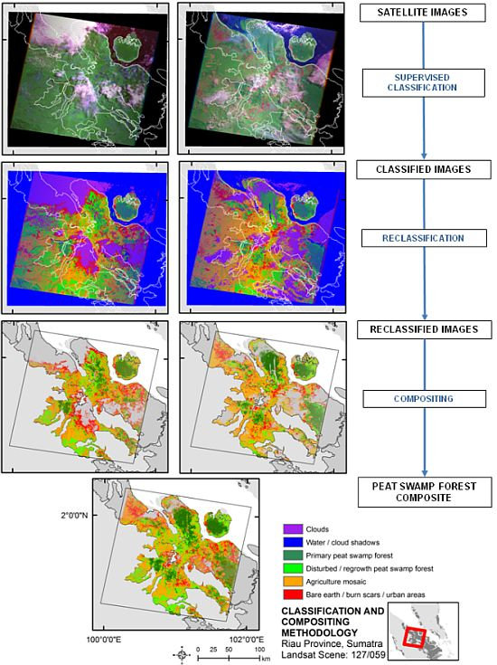
3.4. Map Compositing
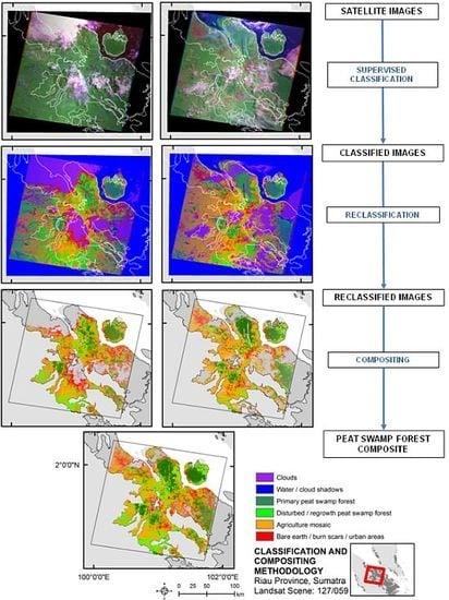
Subsequent to classification, we used a two-step method in ArcMap (Version 9.3) to composite images for 1990, 2000, 2005 and 2010 (Figure 4). First, the land-cover classes in the classified images were assigned the following numerical values, in descending order of disturbance level: 4: primary peat swamp forest, 3: plantation/re-growth, 2: agriculture mosaic, 1: bare earth/urban areas/burn scars, 0: water/cloud shadows/clouds and missing data. For a given scene in 1990, 2000, 2005 and 2010 separately, resultant images were then composited into a single image whereby a given pixel adopted the highest numerical value (and thus corresponding land-cover class) of all coincident pixels. In this way, data gaps in one image due to cloud cover or the SLC-Off errors were filled with data from other cotemporaneous images, where present. As our compositing method uses a ‘maximum’ mosaic operator (i.e., output cell value of the overlapping areas will be the maximum value of the overlapping cells), it prioritizes a ‘forest’ classification over all potential land cover. It therefore partially overlooks the deforestation that occurred between the earliest and latest acquisition dates of the images of a given scene for a given mosaic year, and similarly conservatively estimates forest loss between mosaic years.
Post-classification processing of the composited images was carried out using the majority filter tool in ArcGIS (Version 9.3) using a 3 × 3 kernel This tool serves to reduce ‘speckle’, e.g., isolated pixels of a given class that are probably cases of classification error.
3.5. Accuracy Assessment
Classification accuracy for the composite-image mosaics of 2000, 2005 and 2010 were estimated on a per pixel basis using reference datasets of 662, 741, and 841 randomly generated points for each mosaic, respectively. The points from these reference datasets were randomly sampled in those areas within the original extent of peat swamp forest (defined in Section 3.1) and covered by very high spatial resolution satellite imagery available in Google Earth (e.g., Quickbird, IKONOS) for one of the following periods: 1999–2001, 2004–2006, and 2009–2010 (Figure 5). Independent reference datasets were used for each composite-image mosaic as there was limited overlap in historic imagery available in Google Earth. As high spatial resolution images for ∼1990 were not available in Google Earth, we could not assess the accuracy of the 1990 composite mosaic. However, we expect its accuracy to be comparable to that of later mosaics, given that it was produced with the same data and methods. Similar methods have been used by Miettinen et al. [60] for estimating the accuracy of classifications of plantations on peatlands. In the confusion matrixes of Tables 2–4 we weighted overall classification accuracies based on the proportion of total area accounted for by each land-cover class. This was done to account for the fact that certain land covers have greater proportional areas in the composites. This approach for accuracy assessment is commonly applied to remote sensing products whose land-cover classes have widely varying areas [61].
The land cover of the reference points were visually interpreted in Google Earth as being either peat swamp forests, disturbed/re-growth peat swamp forest, agriculture mosaic, burnt/bare/urban, or undetermined. Points labeled as ‘undetermined’ were those for which the land cover could not be determined due to missing data caused by cloud cover, cloud shadows or the SLC-Off error in either the reference imagery or the composite mosaics. These points were excluded from the accuracy assessment. Thus, although 1,000 reference points were originally sampled for each 2000, 2005, and 2010 mosaics separately, differences in the number of undetermined points for each resulted in slight differences in the number of points used to assess classification accuracies. Tables 2–4 present the results of the comparison of the composite mosaics and the reference data.
3.6. Missing Data
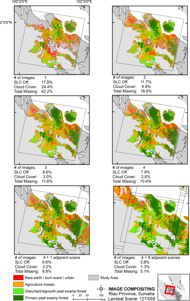
To examine the effect of our image-compositing method on reducing SLC-Off errors and cloud cover, we selected three scenes from the 2010 mosaic which utilized 2, 4 and 6 images (126/060, 127/059 and 124/060). The scenes chosen had similar proportions of study area and were selected to be in the same region (i.e., east coast of Sumatra) of the study area. We compared the extent of missing data due to SLC-Off and cloud cover separately in the original images and after compositing.
4. Results
4.1. Images Needed Per Composite Scene
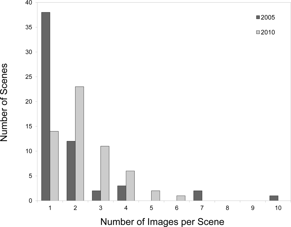
The total number of Landsat images required per scene for the 2005 and 2010 composite mosaics was higher for 2010 mosaic (105 and 133 images, respectively). On average, 1.8 and 2.3 images per scene were required for the 2005 and 2010 composite mosaics respectively to reduce missing data to a level comparable to that of the enhanced 1990 and 2000 mosaics (Figure 6; see Section 4.2). For the 2005 composite made using a combination of Landsat-5 and SLC-off Landsat-7 images (45 and 60 images, respectively), 86% of the scenes required one or two images, while 14% of the scenes required three or more images. In the 2010 composite made using only SLC-Off Landsat-7 images, 64% of the scenes required one or two images and 36% of the scenes required three or more images. The principal reason for this shift in number of images needed per scene, was the availability of 45 Landsat-5 images in the 2005 composite mosaic, while none were available for the 2010 composite mosaic at the time of this study (December 2010).
It is notable that, for the 2010 composite mosaic, the fourteen scenes that required only one image had relatively little remaining peat swamp cover. Indeed, there was a significant positive correlation (Pearson’s r = 0.43; p < 0.001; n = 58 scenes) between the area of remaining peat swamp forest in a given scene and the number of images required of the composite of that scene, notwithstanding spatial variation in cloud cover. This is in keeping with our argument that SLC-Off Landsat imagery retains a utility for monitoring the smaller, fragmented patches of South East Asian peat swamp forests.
As mentioned, the exact number of images composited into a given scene of the 1990 or 2000 mosaics is unknown. Therefore, we estimated the number of images per scene for these mosaics by considering the subset of 32 scenes of the 2005 composite mosaic composed using only of Landsat-5 imagery (i.e., lacking the SLC-Off error). For these 32 scenes, only 1 scene needed 2 images; all other scenes needed only a single image to attain missing-data areas to levels similar to those of the enhanced GeoCover 1990 and 2000 mosaics.
4.2. Extent of Missing Data
For the enhanced 1990 and 2000 composite mosaics, 7.8% and 10.3% of the study area (i.e., original extent of peat swamp forest cover) had missing information due to cloud cover and shadows. In comparison, for the 2005 and 2010 composite mosaics incorporating Landsat-7 SLC-Off images, 8.2% and 8.3% of the study area had missing information due to cloud, shadow, and the SLC-Off error. As such, the extent of missing data is effectively similar across the four composite mosaics, in spite of the SLC-Off problem inherent to Landsat-7 imagery since 2003.
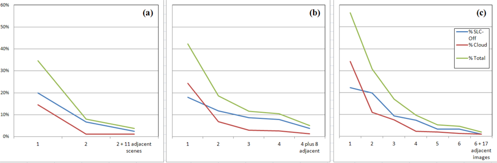
The rate of missing-data reduction per image composited is highly non-linear and exhibits differences for missing-data due to cloud cover versus that due to the SLC-Off error (Figure 7(a–c), Figure 8). Generally, missing-data areas due to cloud cover are reduced much faster per image composited than missing-data areas due to the SLC-Off error. Correspondingly, while cloud cover in a given scene may decline to ∼10% of the study area when only two images are composited, three or four images may generally be required to reduce the total missing-data area to this level (Figure 7, Figure 8). Put differently, most of the initial reduction in missing-data area is relatively large and largely due to declines in cloud cover, and thereafter most reductions will be relatively moderate and largely due to declines in the SLC-error area. Our observations indicate that once a composite scene includes 3 or 4 images and thus attains ∼≥90% coverage of its study area, the additional absolute reduction in missing data upon the inclusion of adjacent, partially overlapping images is relatively moderate, although not insignificant. However, where a regional mosaic of composite scenes is ultimately desired, such gains in spatial coverage are effectively ‘free’ and therefore worth pursuing. Efficiencies in terms of cumulative missing-data reduction per images composited may conceivably be increased across multiple scenes if adjacent images were included in a given composite at the approximate point at which the rate of total-error reduction were expected to flatten a priori (e.g., after compositing the 3rd image in Figure 7(b) or 5th image in Figure 7(c)).
4.3. Error Estimation
The area-weighted overall accuracy of the 2000, 2005 and 2010 composite mosaics ranged from 77% to 86% (Tables 2–4). The producer’s accuracy was generally high for all land-cover classes, ranging from 79 to 96% for the 2005 mosaic and 71–97% for the 2010 mosaic. For the 2000 mosaic a low producer’s accuracy of 56% for the agriculture mosaic class was observed, and probably attributable to the appreciable heterogeneity of the land-use types inherent to this land-cover class. With the exception of the disturbed/regrowth peat swamp forest class, all classes had user’s accuracy ranging from 68 to 86% for 2000, 74 to 88% for 2005 and 79 to 99% for the 2010 mosaic. The disturbed/re-growth peat swamp forest class had lower user’s accuracies of 53–59%, possibly due to: (1) the chronological difference in acquisition years of Landsat imagery (2009–2010) and Quickbird imagery (2011); (2) seasonal variation in fire activity [62]; (3) inter-annual variation in agricultural clearing and fallowing, being cyclic practices widespread in the region; and (4) the transient nature of this land-cover class, which is frequently converted to agriculture mosaic (on this latter point, see in Tables 2–4 the majority of commission errors due to mis-classification of the agriculture mosaic class as disturbed/regrowth peat swamp forest as well as a drop in the proportion of disturbed/regrowth peat swamp forest class and corresponding increase in the agriculture mosaic class).
5. Discussion
By 2013, the Landsat Data Continuity Mission intends to launch a new satellite with improved spatial coverage and revisit periods [14]. It is therefore prudent to explore the utility of existing Landsat imagery for monitoring long-term changes to peat swamp forest area and biodiversity. We have demonstrated a method of compositing classified Landsat images into an accurate regional mosaic that fully utilizes images blighted by cloud cover and SLC-off errors and which produces estimates that are comparable over time. Further, our approach carries certain advantages compared to other, largely pre-classification approaches to Landsat-image composition [14,23,36], namely methodological simplicity and the elimination of the combination of reflectance values of image segments acquired in differing seasons within a given scene.
Most remote-sensing studies that have conducted large-scale mapping of South East Asian peat swamp forests have favored the use of MODIS imagery [6,10–13], no doubt in part due to its relatively cloud-free views and in part due its lack SLC-Off type errors. This preponderance of MODIS-based studies has naturally informed estimates of peat swamp biodiversity decline. For example, both Koh et al. [58] and Giam et al. [63] employ forest matrix-calibrated species-area models utilizing estimates of changes in peat swamp forest cover derived from MODIS classifications to estimate bird and fish species extinctions within Sundaland.
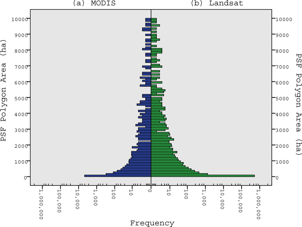
While moderate-resolution imagery such as MODIS is useful for establishing regional trends in forest-cover change, Landsat still has utility for monitoring regional forest trends where forests are highly biodiverse and increasingly fragmented and thus where further perturbations (e.g., logging roads) carry increasingly high biodiversity costs. Observe, for example in Figure 9 how our Landsat composite mosaic of 2000 detects logging roads, appearing as straight narrow lines crisscrossing the primary peat swamp forest on the mainland. Next, observe in Figure 9 how initial perturbations to peat swamp forest on the island’s south east coast whereas a comparable MODIS classification of 2000 [11] does not, and how these perturbed areas appear ‘suddenly’ cleared by 2010 in a later MODIS classification. Lastly, observe in Figure 10 the markedly large proportion of total peat swamp forest area accounted for by smaller fragments across the study region, and how our Landsat composite mosaic of 2000 captures a greater number of these up to approximately 2000 ha compared to the MODIS classification of 2000 (NB. Here all figures concerning the MODIS classifications pertain to study area defined in Section 3.1).
Many of the smallest of these fragments were probably detected only by the Landsat composite given the coarser resolution of the MODIS sensor—indeed, the 2000 Landsat composite mosaic detected 652,476 ha of peat swamp forest over 526,700 patches between 0.36 ha (or 4 contiguous Landsat pixels) and 6.25 ha (or one MODIS pixel). While such diminutive patches constitute only a fraction (7.3%) of the total peat swamp forest area estimated by the 2000 Landsat composite mosaic, fragments of moderate dimensions are still of importance, e.g., patches ≤ 25 ha (or 4 contiguous MODIS pixels) account for 14% of the total peat swamp forest area observed in the 2000 Landsat composite mosaic. Probably more important, however, is the fragmentation that moderate-resolution classifications may overlook. For example, whereas the 2000 MODIS classification observes ∼50% of its total peat swamp forest area amongst 46 patches of between 14,231 ha and 188,360 ha (25th and 75th area quartiles), when clipped to the extent of these 46 patches, our 2000 Landsat composite mosaic detected 873 peat swamp forest patches ≥25 ha within the same area, 512 of which were ≥50 ha, 297 of which were ≥100 ha, 86 of which were ≥1,000 ha, and 49 of which were ≥10,000 ha. Considering therefore on the one hand, the centrality of estimates of forest area and fragmentation to models of biodiversity decline such as those of Koh et al. and [58] and Giam et al. [63] and, and on the other hand, the demonstrated potential of Landsat composite mosaics to regionally monitor fragmented forests of high conservation value, we contend that such mosaics represent an attractive and reliable basis for regional conservation prioritization and estimation of peat swamp forest biodiversity declines.
As mentioned, our estimates of peat swamp forest cover are conservative, as our compositing algorithm prioritizes peat swamp forest over alternative land covers wherever there is discrepancy amongst pixels of input classified images. Correspondingly, for a given nominal year, the estimated peat swamp forest cover is probably slightly greater than reality. Similarly, the extent of deforestation/degradation between nominal years is probably slightly less than reality. Our particular prioritization served to minimize the confounding effects oil-palm plantation misclassified as forest regrowth, but was otherwise arbitrary, and alternative decision rules would doubtlessly elevate the footprint of non-peat swamp forest cover in a similar manner. Future research should explore the sensitivity of our estimates to alternative decision rules.
6. Conclusion
Our results show that despite ∼25% of lost data due to the SLC-off error in Landsat-7 imagery, 85% of the scenes mapped using solely SLC-Off Landsat images in our 2010 and 2005 composite mosaics of Sundaland required only one-to-three images to reduce the extent of missing data to levels comparable to those of the 1990 and 2000 composite mosaics, at ∼8–10%. The apparent ease with which the 2005 and 2010 composite mosaics were rendered comparable to earlier composite mosaics owed in large part to the fact that only a fraction of a given scene was of interest, namely the original extent of peat swamp forest, effectively reducing the cloud-free area required per image. As such, while multi-decadal time-series Landsat mosaics may not be appropriate for tropical forest monitoring for all contexts [18], we believe that they are both appropriate and feasible for monitoring the fragmented and dispersed areas of Sundaland’s peat swamp forests.
Acknowledgments
We are grateful to Jack Dangermond, Leslie Wong, Frankie Loh and ESRI Singapore for a grant of ArcGIS licenses to the Singapore Botanic Gardens. We also thank Neil Stuart, Iain Woodhouse, Iain Cameron and three anonymous reviewers whose comments greatly improved the manuscript. Finally, we thank Greg Asner and William F. Laurance for inviting us to submit this paper for this special issue. G.R. Clements is supported by a James Cook University Postgraduate Research Scholarship and University of Malaya Research Grant. S. Sloan is supported by the ARC Laureate Grant of William F. Laurance. D. Michelakis is supported by an IKY Scholarship from the resources of O.P. “Education and lifelong Learning”, European Social Fund (ESF) and the NSRF 2007–2013.
References and Notes
- Posa, M.R.C.; Wijedasa, L.S.; Corlett, R.T. Biodiversity and conservation of tropical peat swamp forest. BioScience 2011, 61, 49–57. [Google Scholar]
- Page, S.E.; Wust, R.A.; Weiss, J.; Rieley, J.O.; Shotyk, W; Limin, S.H. A record of late Pleistocene and Holocene carbon accumulation and climate change from an equatorial bog (Kalimantan, Indonesia): Implications for past, present and future carbon dynamics. J. Quart. Sci 2004, 19, 625–635. [Google Scholar]
- Jaenicke, J.; Rieley, J.O.; Mott, C.; Kimman, P.; Siegert, F. Determination of the amount of carbon stored in Indonesian peatlands. Geoderma 2008, 47, 151–158. [Google Scholar]
- Page, S.E.; Siegert, F.; Böhm, H-D.V.; Jaya, A.; Limin, S. The amount of carbon released from peat and forest fires in Indonesia in 1997. Nature 2002, 420, 61–65. [Google Scholar]
- Page, S.E.; Rieley, J.O.; Banks, C.J. Global and regional importance of the tropical peatland carbon pool. Glob. Change Biol 2011, 17, 798–818. [Google Scholar]
- Miettinen, J.; Shi, C.; Liew, S.C. Two decades of destruction in Southeast Asia’s peat swamps. Front. Ecol. Environ 2012, 10, 124–128. [Google Scholar]
- Friess, D.A.; Webb, E.L. Bad data equals bad policy: How to trust estimates of ecosystem loss when there is so much uncertainty? Environ. Conserv 2011, 38, 1–5. [Google Scholar]
- Hansen, M.C.; Stehman, S.V.; Potapov, P.V. Quantification of global gross forest cover loss. Proc. Natl. Acad. Sci. USA 2010, 107, 8650–8655. [Google Scholar]
- Uryu, Y.; Mott, C.; Foead, N.; Yulianto, K.; Budiman, A.; Setiabudi; Takakai, F.; Nursamsu, S.; Purastuti, E.; Fadhli, N.; et al. Deforestation, Forest Degradation, Biodiversity Loss and CO2 Emissions in Riau, Sumatra, Indonesia; Technical Report; WWF Indonesia: Jakarta, Indonesia, 2008. [Google Scholar]
- Langner, A.; Miettinen, J.; Siegert, F. Land cover change 2002–2005 in Borneo and the role of fire derived from MODIS imagery. Glob. Change Biol 2007, 13, 2329–2340. [Google Scholar]
- Miettinen, J.; Shi, C.; Tan, W.J.; Liew, S.C. 2010 land cover map of insular Southeast Asia in 250m spatial resolution. Remote Sens. Lett 2012, 3, 11–20. [Google Scholar]
- Miettinen, J.; Wong, C.M.; Liew, S.C. New 500m spatial resolution land cover map of the western insular Southeast Asia region. Int. J. Remote Sens 2008, 29, 6075–6081. [Google Scholar]
- Miettinen, J.; Shi, C.; Liew, S.C. Deforestation rates in insular Southeast Asia between 2000 and 2010. Glob. Change Biol 2011, 17, 2261–2270. [Google Scholar]
- Wulder, M.A.; White, J.C.; Masek, J.G.; Dwyer, J.; Roy, D.P. Continuity of Landsat observations: Short term considerations. Remote Sens. Environ 2011, 115, 747–751. [Google Scholar]
- Hansen, M.C.; Stehman, S.V.; Potapov, P.V. Quantification of global gross forest cover loss. Proc. Natl. Acad. Sci. USA 2010, 107, 8650–8655. [Google Scholar]
- Sloan, S. Historical tropical successional forest mapped with Landsat MSS imagery. Int. J. Remote Sens 2012, in press.. [Google Scholar]
- Walker, W.S.; Stickler, C.M.; Kellndorfer, J.M.; Kirsch, K.M.; Nepstad, D.C. Large-area classification and mapping of forest and land cover in the Brazilian Amazon: A comparative analysis of ALOS/PALSAR and Landsat data sources. IEEE J. Sel. Top. Appl 2010, 3, 594–604. [Google Scholar]
- Broich, M.; Hansen, M.C.; Potapov, P.; Adusei, B.; Lindquist, E.; Stehman, S.V. Time-series analysis of multi-resolution optical imagery for quantifying forest cover loss in Sumatra and Kalimantan, Indonesia. Int. J. Appl. Earth Obs 2011, 13, 277–291. [Google Scholar]
- Asner, G. Cloud cover in Landsat observations of the Brazilian Amazon. Int. J. Remote Sens 2001, 22, 3855–3862. [Google Scholar]
- Nezry, E.; Mougin, E.; Lopes, A.; Gastellu-Etchegorry, J.P. Tropical vegetation mapping with combined visible and SAR spareborne data. Int. J. Remote Sens 1993, 14, 2165–2184. [Google Scholar]
- Storey, J.P.; Scaramuzza, G.; Schmidt, J.B. Landsat-7 Scan Line Corrector-Off Gap Filled Product Development. Proceedings of Pecora 16 Global Priorities in Land Remote Sensing, Sioux Falls, SD, USA, 23–27 October 2005.
- Trigg, S.N.; Curran, L.M.; McDonald, A.K. Utility of Landsat-7 satellite data for continued monitoring of forest cover change in protected areas in Southeast Asia. Singapore J. Trop. Geo 2006, 27, 49–66. [Google Scholar]
- Wulder, M. A.; Ortlepp, S. M.; White, J.C.; Maxwell, S. Evaluation of Landsat-7 SLC-off image products for forests change detection. Can. J. Remote Sens 2008, 34, 93–99. [Google Scholar]
- Chen, J.; Zhu, X; Vogelmann, J.E.; Gao, F.; Jin, S. A simple and effective method for filling gaps in Landsat ETM+ SLC-off images. Remote Sens. Environ 2011, 115, 1053–1064. [Google Scholar]
- Hansen, M.C.; Roy, D.P.; Lindquist, E.; Adusei, B.; Justice, C.O.; Altstatt, A. A method of integrating MODIS and Landsat data for systematic monitoring of forest cover and change in the Congo Basin. Remote Sens. Environ 2008, 112, 2495–2513. [Google Scholar]
- Tuomisto, H; Linna, A.; Kalliola, R. Use of digitally processed satellite images in studies of tropical rain forest vegetation. Int. J. Remote Sens 1994, 15, 1595–1610. [Google Scholar]
- Tuomisto, H; Ruokolainen, K.; Kalliola, R.; Linna, A.; Danjoy, W.; Rodriguez, Z. Dissecting Amazonian biodiversity. Science 1995, 269, 63–66. [Google Scholar]
- Tuomisto, H. What satellite imagery and large-scale field studies can tell about biodiversity patterns in Amazonian forests. Ann. Mo. Bot. Gard 1998, 85, 48–62. [Google Scholar]
- Nagendra, H.; Rocchini, D.; Ghate, R.; Sharma, B.; Pareeth, S. Assessing plant diversity in a dry tropical forest: comparing the utility of Landsat and IKONOS satellite images. Remote Sens 2010, 2, 478–496. [Google Scholar]
- Eva, H.D.; Achard, F.; Beuchle, R.; de Miranda, E.; Carboni, S.; Seliger, R.; Vollmar, M.; Holler, W.A.; Oshiro, O.T.; Arroyo, V.B.; Gallego, J. Forest cover changes in tropical South and Central America from 1990 and 2005 and related carbon emissions and removals. Remote Sens 2012, 4, 1369–1391. [Google Scholar]
- Gervin, J.C.; Kerber, A.G.; Witt, R.G.; Lu, Y.C.; Sekhon, R. Comparison of level I land cover classification accuracy for MSS and AVHRR data. Int. J. Remote Sens 1985, 6, 47–57. [Google Scholar]
- Laporte, N.T.; Stabach, J.A.; Grosch, R.; Lin, T.S.; Goetz, S.J. Expansion of industrial logging in Central Africa. Science 2007, 316, 1451. [Google Scholar]
- Brandão, A.O., Jr.; Souza, C.M., Jr. Mapping unofficial roads with Landsat images: A new tool to improve the monitoring of the Brazilian Amazon rainforest. Int. J. Remote Sens 2006, 27, 177–189. [Google Scholar]
- Brook, B.; Bradshaw, C.A.; Koh, L.P.; Sodhi, N.S. Momentum drives the crash: Mass extinction in the Tropics. Biotropica 2006, 38, 302–305. [Google Scholar]
- Lindquist, E.J.; Hansen, M.C.; Roy, D.P.; Justice, C.O. The suitability of decadal image data sets for mapping tropical forest change in the Democratic Republic of Congo: Implications for the global land survey. Int. J. Remote Sens 2008, 29, 7269–7275. [Google Scholar]
- Roy, D.P.; Ju, J.; Kline, K.; Scaramuzza, P.L.; Kovalskyy, V.; Hansen, M.; Loveland, T.R.; Vermote, E.; Zhang, C. Web-enabled Landsat Data (WELD): Landsat ETM+ composited mosaics of the conterminous United States. Remote Sens. Environ 2010, 114, 35–49. [Google Scholar]
- Roy, D.P.; Ju, J.; Lewis, P.; Schaaf, C.; Gao, F.; Hansen, M.; Lindquist, E. Multi-temporal MODIS-Landsat data fusion for relative radiometric normalization, gap filling and prediction of Landsat data. Remote Sens. Environ 2008, 112, 3112–3130. [Google Scholar]
- Staff of the Soils and Analytical Services Branch. Division of Agriculture. Ministry of Agriculture and Fisheries, Malaysia under the Supervision of Law, W.M. Reconnaissance Soil Map of Peninsular Malaysia. Sheet 1. Series L 40A; Directorate of National Mapping: Kuala Lumpur, Malaysia, 1968; Scale: 1:500,000. [Google Scholar]
- Soil Survey Division, Research Branch, Department of Agriculture, Sarawak, with the assistance of the Directorate of National Mapping, Malaysia. Soil Map of Sarawak; Sheets: A & B; Directorate of National Mapping: Kuala Lumpur, Malaysia, 1970; Scale 1: 500,000.
- Directorate of National Mapping, Malaysia. Soils of Sabah. Sheets: NB, NB 50-6, NB 50-7, NB 50-9, NB 50-10, NB 50-11, NB 50-12, NB 50-14, NB 50-15, NB 50-16; The British Government’s Overseas Development Administration (Land Resources Division): London, UK, 1974; Scale 1:250,000. [Google Scholar]
- Center for Soil and Agroclimatic Research. Soil Resource Atlas of Indonesia. Sheets: MA47, MA48, MA49, MB48, MB54, NA47, NA48, NA49, NA50, NB46, NB47 and NB50; Center for Soil and Agroclimatic Research: Bogor, Indonesia, 2000; Scale 1:1,000,000. [Google Scholar]
- Wahyunto; Ritung, S.; Subagjo, H. Maps of Area of Peatland Distribution and Carbon Content in Sumatra, 1990–2002; Wetlands International, Indonesia Programme & Wildlife Habitat Canada (WHC): Bogor, Indonesia, 2003. [Google Scholar]
- Wahyunto; Ritung, S.; Suparto; Subagjo, H. Maps of Area of Peatland Distribution and Carbon Content in Kalimantan, 2000–2002; Wetlands International, Indonesia Programme & Wildlife Habitat Canada (WHC): Bogor, Indonesia, 2004. [Google Scholar]
- Coulter, J.K. Peat formations in Malaya. Malay. Agric. J 1950, 33, 63–81. [Google Scholar]
- Wyatt-Smith, J. Peat swamp forest in Malaya. Malay. For 1959, 22, 5–32. [Google Scholar]
- Anderson, J.A.R. The structure and development of the peat swamps of Sarawak and Brunei. J. Trop. Geogr 1964, 18, 7–16. [Google Scholar]
- Whitmore, T.C. Tropical Rainforests of the Far East; Clarendon Press: Oxford, UK, 1975; p. 281. [Google Scholar]
- Anderson, J.A.R.; Marsden, D. Brunei Forest Resources and Strategic Planning Study; Anderson & Marsden: Singapore, 1984; Scale 1:50, 000. [Google Scholar]
- Laumonier, Y.; Gadrinab, A.; Purnajaya; Blasco, F. International Map of the Vegetation and Environmental Conditions. Sheet No. 1 (Southern Sumatra), Sheet No. 2 (Central Sumatra) and Sheet no. 3 (Northern Sumatra); SEAMEO-BIOTROP: Bogor, Indonesia, 1986; Scale 1:1,000,000. [Google Scholar]
- Anderson, J.A.R. The structure and development of the peat swamps of Sarawak and Brunei. J. Trop. Geogr 1964, 18, 7–16. [Google Scholar]
- Van Steenis, C.G.G.J. Outline of vegetation types in Indonesia and some adjacent regions. Proc. Pacif. Sci. Congr 1957, 8, 61–97. [Google Scholar]
- Wyatt-Smith, J. Manual of Malayan Silviculture for Inland Forests; Malayan Forest Records; Forest Research Institute Malaysia: Kuala Lumpur, Malaysia, 1963; Issue 22. [Google Scholar]
- Director of Lands and Surveys, Sarawak. Sarawak Land Use. Series No. 22. Sheets: NA 49-4, NA 49-7, NA 49-10, NA 49-11, NA 49-12, NA 50-1, NA 50-5, NB 50-13; Directorate of National Mapping: Kuala Lumpur, Malaysia, 1968–1980; Scale 1:25,000. [Google Scholar]
- Land Use Survey section. Soil Science Division. Division of Agriculture. Ministry of Agriculture and Lands, Malaysia. Present Land Use. West Malaysia. Sheet 1 & 2; Directorate of National Mapping: Kuala Lumpur, Malaysia, 1966; Scale 1: 500,000. [Google Scholar]
- UNEP-WCMC. Tropical Moist Forest s and Protected Areas: The Digital Files. Version 1. 1996..
- The Global Land Cover Facility. Landsat Orthorectified Dataset (January 2005– December 2011). 2005. Available online: www.glovis.org (accessed on 31 December 2011).
- USGS. Shuttle Radar Topography Mission, 1 Arc Second scene SRTM_u03_n008e004, Unfilled Unfinished 2.0, Global Land Cover Facility; University of Maryland, College Park: MD, USA, 2004. [Google Scholar]
- Koh, L.P.; Miettinen, J.; Liew, S.C.; Ghazoul, J. Remotely sensed evidence of tropical peatland conversion to oil palm. Proc. Natl. Acad. Sci. USA 2011, 108, 5127–5132. [Google Scholar]
- Steininger, M.K. Tropical secondary regrowth in the Amazon: Age, area and change estimation with Thematic Mapper data. Int. J. Remote Sens 1996, 17, 9–27. [Google Scholar]
- Miettinen, J.; Hooijer, A.; Shi, C.H.; Tollenaar, D.; Vernimmen, R.; Liew, S.C.; Malins, C.; Page, S. Extent of industrial plantations on Southeast Asian peatlands in 2010 with analysis of historical expansion and future projections. GCB Bioenergy 2012. [Google Scholar] [CrossRef]
- Bontemp, S.; Defourny, P.; Van Bogaert, E.; Arino, O.; Kalogirou, V.; Ramos Perez, J. GlobCover 2009: Product Description and Validation Report; Universite Catholoque de Louvain, European Space Agency: Louvain, Belgium, 2011. [Google Scholar]
- Miettinen, J.; Shi, C.; Liew, S.C. Influence of peatland and land cover distribution on fire regimes in insular Southeast Asia. Reg. Environ. Change 2011, 11, 191–201. [Google Scholar]
- Giam, X.; Koh, L.P.; Tan, H.H.; Miettinen, J.; Tan, H.T.W.; Ng, P.K.L. Global extinctions of freshwater fishes follow peatland conversion in Sundaland. Front. Ecol. Environ 2012, in press.. [Google Scholar]
Appendix
Figure A1.
Spatial illustration of missing-data reduction per image when compositing two Landsat-7 SLC-Off images for scene 126/060 of the 2010 composite mosaic. Percentages reported are with respect to the study area, not the entire scene. The mapped area corresponds to Figure 7(a).
Figure A1.
Spatial illustration of missing-data reduction per image when compositing two Landsat-7 SLC-Off images for scene 126/060 of the 2010 composite mosaic. Percentages reported are with respect to the study area, not the entire scene. The mapped area corresponds to Figure 7(a).
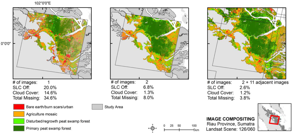
Figure A2.
Spatial illustration of missing-data reduction per image when compositing six Landsat-7 SLC-Off images for scene 124/060 of the 2010 composite mosaic. Percentages reported are with respect to the study area, not the entire scene. The mapped area corresponds to Figure 7(c).
Figure A2.
Spatial illustration of missing-data reduction per image when compositing six Landsat-7 SLC-Off images for scene 124/060 of the 2010 composite mosaic. Percentages reported are with respect to the study area, not the entire scene. The mapped area corresponds to Figure 7(c).

Figure 1.
Example of how Scan-Line Corrector (SLC-Off) error affects Landsat scenes in Riau province, Sumatra. (a) Overlay of four Landsat-7 images with SLC-Off error for scene 127/059 (blue), and one Landsat image with SLC-Off error for scene 126/059 (red); (b–d) close-up views of SLC-OFF missing-data areas across each Landsat scene. Increasing intensity of blue indicates increasing number of scenes with overlaps of missing data due to SLC-Off error. Note that among the four images for scene 127/059, the missing-data stripes only overlap completely in two images (c). At the edge of the scene (d), missing data is further reduced by a 30-km wide overlap with the adjacent scene, visible as red stripes.
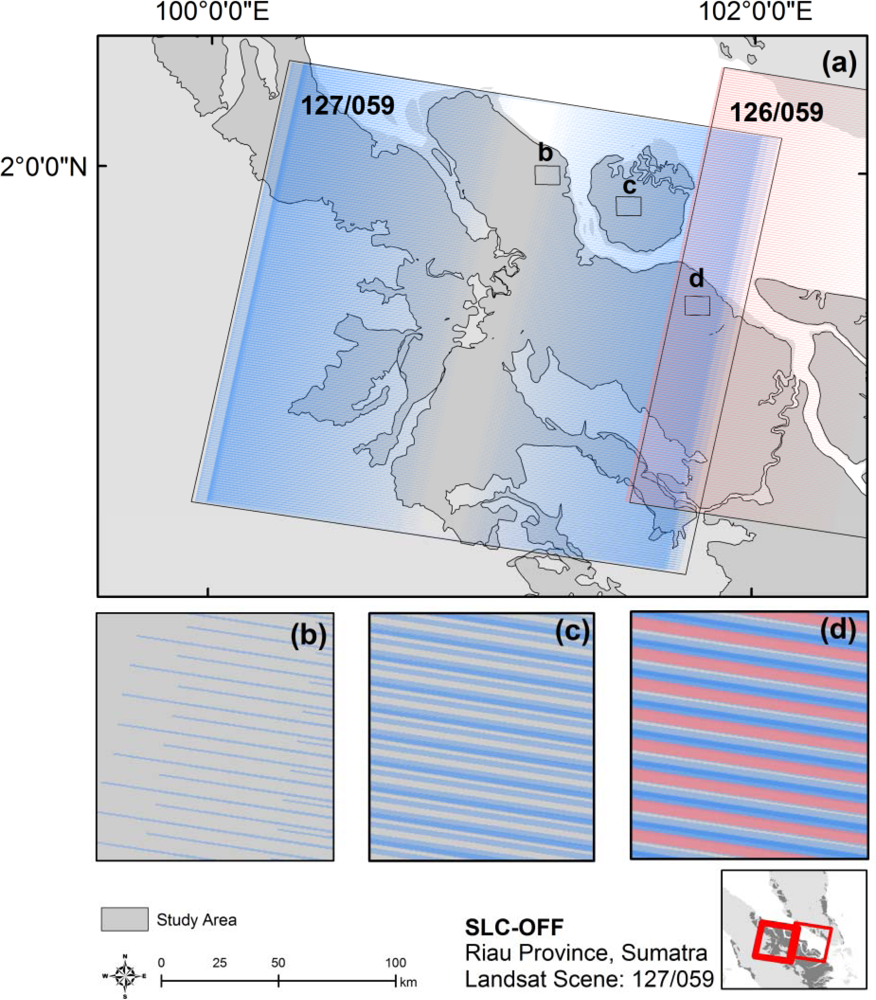
Figure 2.
(a) Map showing the study area and number of images used per scene in the 2005 composite (n = 105 images). (b) Map showing the study area and number of images used per scene in the 2010 composite (n = 133 images). Red areas indicate original peat swamp forest extent.
Figure 2.
(a) Map showing the study area and number of images used per scene in the 2005 composite (n = 105 images). (b) Map showing the study area and number of images used per scene in the 2010 composite (n = 133 images). Red areas indicate original peat swamp forest extent.
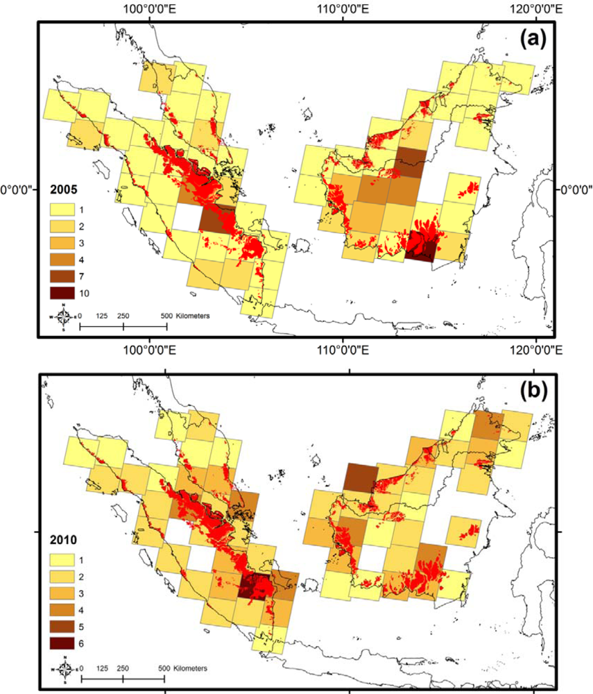
Figure 3.
Land cover classes as represented by training sites: burn scars/bare earth/urban areas (1), agriculture mosaic (2), disturbed /re-growth peat swamp forest (3), primary peat swamp forest (4), cloud cover (5), cloud shadow (6) and water (7). The lines in the image represent missing data due to SLC-Off error.

Figure 4.
Flow diagram of classification and compositing methodology for Landsat scene 127/059. From raw image, classified image, reclassified image and composited image.
Figure 4.
Flow diagram of classification and compositing methodology for Landsat scene 127/059. From raw image, classified image, reclassified image and composited image.

Figure 5.
Areas used for accuracy assessment of the 2000, 2005 and 2010 composites.
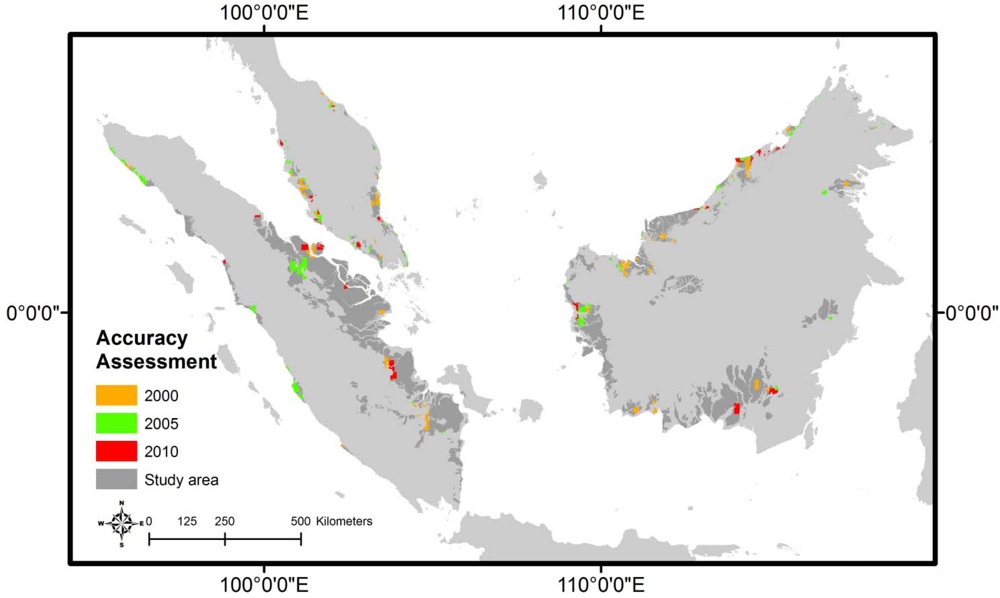
Figure 6.
The number of images composited per scene for 2005 and 2010 composite mosaics. Note the high proportion of scenes requiring three or fewer images. Also note the decreasing proportion of scenes requiring only a single image between 2005 and 2010. This indicates that even though areas of peat swamp forest cover of interest occupy smaller proportions of scenes in 2010 and would potentially require fewer images to be mapped, this is offset by additional missing area due to the SLC-Off error.

Figure 7.
Graphical illustration of missing-data reduction per image when compositing images and adjacent scenes (a) two, (b) four and (c) six Landsat-7 SLC-Off images of the 2010 composite mosaic, plus images of adjacent scenes (corresponding spatial illustrations of these scenes are given in Figure 8 and in the appendix). Percentages reported are with respect to the study area, not the entire scene. The scene path/rows for panes (a), (b) and (c) are 126/060, 127/059, and 124/060, respectively.

Figure 8.
Spatial illustration of missing-data reduction per image when compositing four Landsat-7 SLC-Off images for scene 127/059 of the 2010 composite mosaic. Percentages reported are with respect to the study area, not the entire scene. The mapped area corresponds to Figure 7(b). Equivalent figures corresponding to Figure 7(a,c) are given in the Appendix.

Figure 9.
Comparison of the 2000 and 2010 Landsat mosaics with the corresponding MODIS mosaics of 2000 and 2010 created by Miettinen et al. [11], Northern Riau Province, Sumatra, Indonesia.
Figure 9.
Comparison of the 2000 and 2010 Landsat mosaics with the corresponding MODIS mosaics of 2000 and 2010 created by Miettinen et al. [11], Northern Riau Province, Sumatra, Indonesia.
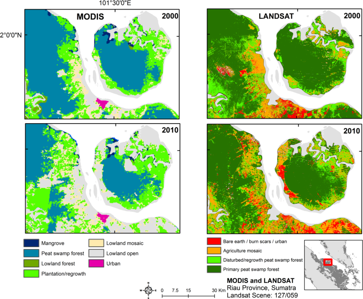
Figure 10.
Distribution of area of peat swamp forest patches in Sundaland, 2000, as observed by the MODIS classification of Miettinen et al. [13] and the Landssat classification of the present study. (NB. We discuss here our composite mosaic of 2000 rather than that of 2010 in order to avoid biases due (i) any ‘artificial’ fragmentation of peat swamp forest patches due to the compositing of SLC-off images, and (ii) the presence of mature oil-palm plantations misclassified as peat swamp forest in 2010).Note: Abbreviation ‘PSF’ means peat swamp forest. Gradations on the x-axis are log10 scaled with 4 minor gradations per major gradation, but labels report actual frequencies. Frequencies are shown for 100-ha cohorts for polygons between 0.36 ha (or 4 contiguous Landsat pixels) and 10,000 ha, where the lower limit minimizes the influence of Landsat classification ‘speckle’ and the upper limit is for the sake of presentation. Both histograms (a) and (b) pertain to the Sundaland study area delimited according to Section 3.1. Miettinen et al. [13] define peat swamp forest similarly to us as forest growing on peat soil, including perturbed forests whose structural characteristics (e.g., height, canopy closure, etc) resemble primary forest. Also, our peat swamp forest classification accuracy is similar to that of Miettinen et al. [13], reported in Miettinen et al. (Table 2 in [11]). The peat swamp forest class of Miettinen et al. [13] is possibly more spatially confined than ours, as Miettinen et al. [11] observe ‘lowland forest’ adjacent to their peat swamp forest polygons where we observe only peat swamp forest.

| Land Cover Type | Description |
|---|---|
| Primary peat swamp forest | Undisturbed peat swamp forest and old re-growth peat swamp forest with little or no disturbance due to logging, conversion or fire. Old re-growth includes some previously logged peat swamp forest that has regenerated and cannot be distinguished from undisturbed peat swamp forest. |
| Disturbed/re-growth peat swamp forest | Peat swamp forest that has been disturbed by logging and fire. Visible as open canopy peat swamp forest with a visibly different texture and reflectance than primary peat swamp forest. This class includes re-growth peat swamp forest which does not have the same reflectance and texture as undisturbed primary peat swamp forest or old re-growth peat swamp forest. |
| Agriculture mosaic | Comprises all non-peat swamp forest land use types except burn scars/bare earth/urban areas. This a heterogeneous class made up mostly of large scale industrial plantations of oil palm and acacia and small holder plantations. Some of the other land use types in this class are open areas with ferns/low shrubs and young regrowth forest. |
| Burn scars/bare earth/urban areas | Urban areas and bare earth. This includes bare earth caused by recently burnt areas. |
| Missing data | SLC-Off areas, clouds, shadows caused by clouds in the image and open water. |
| Reference Dataset | ||||||
|---|---|---|---|---|---|---|
| Landsat Classified Composite | Primary Peat Swamp Forest | Disturbed/Regrowth Peat Swamp Forest | Agriculture Mosaic | Burn Scars/ Bare Earth/ Urban Areas | Total | User’s Accuracy |
| Primary peat swamp forest | 247 | 6 | 32 | 1 | 286 | 86% |
| Disturbed/regrowth peat swamp forest | 25 | 85 | 48 | 2 | 160 | 53% |
| Agriculture mosaic | 19 | 6 | 126 | 0 | 151 | 83% |
| Burn scars/bare earth/urban areas | 2 | 0 | 19 | 44 | 65 | 68% |
| Total | 293 | 97 | 225 | 47 | ||
| Producer’s Accuracy | 84% | 88% | 56% | 94% | ||
| Proportion of Land Cover | 50% | 20% | 20% | 10% | ||
| Weighted Overall Accuracy = 77% | ||||||
| Reference Dataset | ||||||
|---|---|---|---|---|---|---|
| Landsat Classified Composite | Primary peat swamp forest | Disturbed/regrowth peat swamp forest | Agriculture mosaic | Burn scars/ bare earth/ urban areas | Total | User’s Accuracy |
| Primary peat swamp forest | 181 | 13 | 11 | 0 | 205 | 88% |
| Disturbed/regrowth peat swamp forest | 8 | 86 | 51 | 2 | 147 | 59% |
| Agriculture mosaic | 10 | 4 | 286 | 1 | 301 | 95% |
| Burn scars/bare earth/urban areas | 9 | 1 | 13 | 65 | 88 | 74% |
| Total | 208 | 104 | 361 | 68 | 741 | |
| Producer’s Accuracy | 87% | 83% | 79% | 96% | ||
| Proportion of Land Cover | 45% | 19% | 27% | 9% | ||
| Weighted Overall Accuracy = 85% | ||||||
| Reference Dataset | ||||||
|---|---|---|---|---|---|---|
| Landsat Classified Composite | Primary peat swamp forest | Disturbed/regrowth peat swamp forest | Agriculture mosaic | Burn scars/ bare earth/ urban areas | Total | user’s accuracy |
| Primary peat swamp forest | 252 | 12 | 55 | 1 | 320 | 79% |
| Disturbed/regrowth peat swamp forest | 3 | 87 | 63 | 0 | 153 | 57% |
| Agriculture mosaic | 2 | 0 | 303 | 1 | 306 | 99% |
| Burn scars/bare earth/urban areas | 2 | 1 | 3 | 56 | 62 | 90% |
| Total | 259 | 100 | 424 | 58 | ||
| Producer’s Accuracy | 97% | 87% | 71% | 97% | ||
| Proportion of Land Cover | 45% | 14% | 34% | 6% | ||
| Weighted Overall Accuracy = 86% | ||||||
Share and Cite
MDPI and ACS Style
Wijedasa, L.S.; Sloan, S.; Michelakis, D.G.; Clements, G.R. Overcoming Limitations with Landsat Imagery for Mapping of Peat Swamp Forests in Sundaland. Remote Sens. 2012, 4, 2595-2618. https://doi.org/10.3390/rs4092595
AMA Style
Wijedasa LS, Sloan S, Michelakis DG, Clements GR. Overcoming Limitations with Landsat Imagery for Mapping of Peat Swamp Forests in Sundaland. Remote Sensing. 2012; 4(9):2595-2618. https://doi.org/10.3390/rs4092595
Chicago/Turabian StyleWijedasa, Lahiru S., Sean Sloan, Dimitrios G. Michelakis, and Gopalasamy R. Clements. 2012. "Overcoming Limitations with Landsat Imagery for Mapping of Peat Swamp Forests in Sundaland" Remote Sensing 4, no. 9: 2595-2618. https://doi.org/10.3390/rs4092595