Remote Sensing of Fractional Green Vegetation Cover Using Spatially-Interpolated Endmembers

Center for Environmental Remote Sensing (CEReS), Chiba University, 1-33 Yayo-icho, Inage, Chiba 263-8522, Japan
*
Author to whom correspondence should be addressed.
Remote Sens. 2012, 4(9), 2619-2634; https://doi.org/10.3390/rs4092619
Submission received: 27 July 2012
/
Revised: 3 September 2012
/
Accepted: 4 September 2012
/
Published: 12 September 2012
Abstract
:Fractional green vegetation cover (FVC) is a useful parameter for many environmental and climate-related applications. A common approach for estimating FVC involves the linear unmixing of two spectral endmembers in a remote sensing image; bare soil and green vegetation. The spectral properties of these two endmembers are typically determined based on field measurements, estimated using additional data sources (e.g., soil databases or land cover maps), or extracted directly from the imagery. Most FVC estimation approaches do not consider that the spectral properties of endmembers may vary across space. However, due to local differences in climate, soil type, vegetation species, etc., the spectral characteristics of soil and green vegetation may exhibit positive spatial autocorrelation. When this is the case, it may be useful to take these local variations into account for estimating FVC. In this study, spatial interpolation (Inverse Distance Weighting and Ordinary Kriging) was used to predict variations in the spectral characteristics of bare soil and green vegetation across space. When the spatially-interpolated values were used in place of scene-invariant endmember values to estimate FVC in an Advanced Spaceborne Thermal Emission and Reflection Radiometer (ASTER) image, the accuracy of FVC estimates increased, providing evidence that it may be useful to consider the effects of spatial autocorrelation for spectral mixture analysis.
1. Introduction
In medium-to-coarse spatial resolution satellite images, single pixels often contain a mixture of different types of land cover. Use of very high resolution imagery can mitigate this mixed pixel problem to some degree, but the relatively higher cost and lower frequency at which high resolution imagery is typically acquired can be an issue. On the other hand, Spectral Mixture Analysis (SMA) provides a method to estimate the fractional abundance of the different types of land cover within medium-to-coarse resolution pixels based on the spectral characteristics of spectrally-pure “endmembers”, which are representative of each land cover type [1]. Of particular importance for many applications including soil erosion risk assessment [2], climate and hydrologic modeling [3–5], severe weather forecasting [6], and land surface temperature retrieval [7] is fractional green vegetation cover (FVC); the fraction of green vegetation within a pixel. A number of remote sensing studies have estimated FVC in multispectral or hyperspectral images using a Linear Spectral Unmixing (LSU) approach with two or more endmembers [2–5,7–12]. Non-linear unmixing approaches also exist (e.g., [13–15]), but the linear approach is used most often due to its simplicity, rationality, and feasibility in practical applications [16]. The number of spectral bands in an image limits the number of endmembers that can be used for unmixing [17], so for images with relatively few spectral bands, a common approach is to assume that FVC can be estimated by the linear combination of two endmembers: bare soil and 100% green vegetation cover [3,6,7,12,18]. In this two endmember model, it is also typically assumed that dead vegetation is spectrally-similar to bare soil [3], although [19] found that surface albedo can be used to separate soil and dead vegetation in areas with low-albedo soils. A commonly-used linear model for deriving FVC from spectral Vegetation Index (VI) values, referred to as the VI-based linear mixture model [16], is described in Gutman and Ignatov [3] as
where VIi is the VI value of pixel i, VIs is the VI of bare soil or dead vegetation pixels in the image (i.e., no green vegetation cover), and VIv is the VI of fully-vegetated pixels. Appropriate VIs and VIv endmembers are typically obtained from previous studies or soil databases [5,7], or directly from the imagery using various techniques [4,5,7]. Many studies estimate FVC under the assumption that VIs and/or VIv are invariant throughout an image (e.g., [3,4,7,8]). However, this assumption is often invalid [5] because differences in soil composition, grain size, and moisture content can cause the spectral characteristics of soil to vary [20], and differences in vegetation species, leaf water content, etc. can cause the spectral characteristics of green vegetation to vary [21]. In areas with rugged terrain, the effects of topography (i.e., differences in solar illumination on slopes oriented towards and away from the sun) also have an impact on spectral reflectance values of soil and green vegetation [22].
To deal with the variability in VIs, a popular approach has been to use vegetation indices less sensitive to soil brightness than NDVI, such as the Soil Adjusted Vegetation Index (SAVI) [23]. In an alternative approach, [5] used a global soil reflectance database (2,906 soil reflectance samples), computed many possible FVC values for each pixel using different NDVIs values from the soil database (i.e., using all soil samples with NDVI values lower than the NDVI of the pixel), and assigned the mean FVC of these calculations to the pixel since it was the statistically most-likely. This method was able to increase the accuracy of FVC estimates for the continental United States, but for studies conducted at finer scales the majority of the soils in a global database may not be present, so the approach lacks a physical basis for these fine-scale studies.
To deal with the spatial variability in VIv, some studies have used land cover maps to derive separate VIv values for each type of vegetation [4,24]. This approach provides a way to account for some of the variability in VIv, but: (i) land cover maps of the desired classification accuracy or spatial resolution may not always be available, and (ii) it does not take into consideration the local climate and soil conditions which can cause spectral characteristics even at the species level to vary across space [25]. Thus, VIv values may still vary across space even if they are defined for each type of vegetation. In addition, it is possible that VIs may vary as well due to local differences in soil composition and soil moisture. For dealing with the positive spatial autocorrelation likely to exist in VIs and VIv, [10] suggest that subdividing the landscape into several units and developing/applying separate unmixing models for each unit may produce better results, but determining the number and size of the units for dividing the landscape would likely be difficult and subjective. On the other hand, a less subjective approach that also takes into account the likely spatial autocorrelation in VIs and VIv is to use spatial interpolation to predict the variation in VIs and VIv across space. Such an approach was developed in this paper.
The objective of this study was to test the use of spatial interpolation techniques for predicting the variation in VIs and VIv in an image. Two interpolation techniques, Inverse Distance Weighting (IDW) and Ordinary Kriging (OK), were tested. The basic approach is as follows: (i) VIs and VIv values at sample locations were extracted from the imagery (i.e., from manually-selected “bare soil” and “full green vegetation” endmember pixels), (ii) VIs and VIv values at all other pixel locations were predicted by spatially interpolating the VIs and VIv values from the endmember pixels, and (iii) interpolated VIs and VIv replaced the VIs and VIv values used in the traditional linear FVC calculation shown in equation 1. The theoretical basis for the proposed approach is that, at a given location, the spectral characteristics of soil are likely to be more similar to nearer “bare soil” sample endmember pixels and the spectral characteristics of vegetation are likely to be more similar to nearer “full green vegetation” sample endmember pixels due to local similarities in soil and vegetation composition, moisture, etc. Therefore, local calculations of VIs and VIv should provide better estimates of the expected endmember values at each pixel location than globally-invariant VIs and VIv values. Two well-established vegetation indices, the Normalized Differential Vegetation Index (NDVI) [26] and the Modified Soil Adjusted Vegetation Index (MSAVI) [27], were used for the FVC calculations. Very high spatial resolution imagery was used for assessing the accuracy of FVC estimates, and FVC estimates calculated using the spatially interpolated VIs and VIv approach were compared with estimates calculated using the traditional approach (i.e., with invariant VIs and VIv values) to assess the impact that the interpolation approach had on the accuracy of estimates. The accuracy of FVC estimates was assessed for an entire validation dataset (100 validation samples), and also for edge- and non-edge validation samples separately in order to provide a broad view of the spatial distribution of FVC estimation errors in a patchy landscape (i.e., a landscape in which large changes in vegetation cover can occur over short distances).
2. Study Area and Data
The methods proposed in this study were applied for mapping FVC in a forested area of Ibaraki Prefecture, Japan. The study area consists of conifer plantations of Cryptomeria japonica (Japanese cedar) and Chamaecyparis obtusa (Japanese cypress), natural deciduous broadleaf forest, clear cut areas, and a small amount non-forest land use/land cover (e.g., built-up surfaces and agricultural fields). The density of conifers within the tree plantations, which is affected by human activities such as thinning as well as natural causes such as snow damage [28], is inversely related to the abundance of native deciduous broadleaf species also present in these plantations [29]. Since a major goal of Japan’s Forestry Agency is to ensure biodiversity conservation in the tree plantations, which make up 40% of the country’s total forested area [30], information related to conifer tree density within the plantations is important for forest management purposes. In this region of Japan, only the conifer tree species keep their leaves in winter, so mapping of FVC in the winter season can provide an estimate of conifer tree density in these plantations (higher FVC indicates higher conifer density). Orthorectified Advanced Spaceborne Thermal Emission and Reflection Radiometer (ASTER) imagery of the study area was obtained for the image date 19 March 2011 from the Land Processes Distributed Active Archive Center (LP DAAC) at the US Geological Survey (USGS). A false color composite of the study area image is shown in Figure 1. For this study, the 15 m resolution red (0.63–0.69 μm) and NIR (0.76–0.86 μm) ASTER image bands were used for calculating vegetation indices. 50 cm pansharpened true color GeoEye-1 imagery from 18 March 2011, freely available for viewing in Google Earth and Bing Maps, was used to assess the accuracy of FVC estimates.
3. Methods
3.1. Atmospheric and Geometric Correction
Prior to calculating FVC, digital number (DN) values in the ASTER image were converted to at-sensor radiance by multiplying the DN values of each band by their appropriate gains (provided in the image metadata). Then, atmospheric correction of these radiance values was done using the empirical line method [31] with a dark and bright land cover target. The darkest pixels in the image were located completely in shadow, so we located an area in the image with a large number of adjacent shadow pixels (to minimize diffuse reflection from nearby surfaces) and assumed the reflectance of these pixels to be 1% based on [32]. The bright target in the image was snow, and its reflectance was assumed to be that of “coarse granular snow” in the John Hopkins University spectral library [33]. After deriving at-surface reflectance, the ASTER image was overlaid on the high resolution GeoEye-1 imagery in ArcMap 10 using the “Add Basemap” function, which allows for imagery from the Bing Maps database to be viewed in ArcMap, and the ASTER image was coregistered to the high resolution image to sub-pixel accuracy (RMSE of 8.27 m).
3.2. Calculation of Vegetation Indices
After atmospheric and geometric correction, two vegetation indices, NDVI and MSAVI, were calculated. NDVI was calculated as
where NIR is the spectral reflectance of ASTER band 3 and R is that of ASTER band 2. NDVI was chosen for this study because of its wide use for FVC mapping, including its use in global datasets such as the National Oceanic and Atmospheric Administration (NOAA) Fractional Vegetation product ( http://www.ospo.noaa.gov/Products/land/gvi/FRV.html, last accessed on 12 Septermber 2012). MSAVI was calculated as
where NIR and R are ASTER bands 3 and 2, respectively. This MSAVI formula, proposed by [27], was designed to be less sensitive to changes in soil brightness than NDVI, and its advantage over the also commonly-used SAVI comes from the fact that it does not require a soil brightness dependence factor (L) to be manually selected, making it more objective. As can be seen in Figure 1, topographic effects had an impact on ASTER reflectance values in mountainous parts of the study area (e.g., dark areas with low solar illumination are easy to identify). However, in the NDVI and MSAVI images of the study area shown in Figure 2, these topographic effects are not apparent. Thus, we determined that errors in FVC estimates due to topography were likely to be minimal for our study area.
3.3. Calculation of VIs and VIv at Each Sample Location
After the vegetation indices were created, sample locations in the ASTER image containing bare soil and/or dead vegetation (“gv_0” pixels) and full green vegetation cover (“gv_1” pixels) were selected from across the study area (around 50 sample locations each), and high resolution GeoEye-1 imagery was used to confirm that the ASTER pixels at these sample locations were unmixed. To allow for accurate spatial interpolation (rather than extrapolation), we chose sample locations that were widely distributed throughout the entire image, and the spatial distribution of these gv_0 and gv_1 samples can be seen in Figure 3(a,b). At each sample location, the mean NDVI and MSAVI values of the pixels within a 3 × 3 window were calculated, and these mean values were used as the NDVIs and MSAVIs or NDVIv and MSAVIv values (depending on whether the sample was of gv_0 or gv_1) for that location. To determine if the VIs and VIv values exhibited positive spatial autocorrelation for either vegetation index, we computed Global Moran’s I (MI) [34], a metric that calculates, on average, how similar a sample is to other nearby samples. MI was calculated as
where n is the total number of samples, wij is a measure of spatial proximity (measured using IDW), yi is the value of sample i, and ȳ is the mean value of all of the samples.
indicates positive spatial autocorrelation, and
indicates negative spatial autocorrelation. In addition to MI, p values, which give the confidence level for the MI calculations, were also calculated (e.g.,
and p < 0.05 indicates positive spatial autocorrelation at a 95% confidence level). As shown in Table 1, NDVIs and MSAVIs both showed strong positive spatial autocorrelation at a 95% confidence level, while NDVIv and MSAVIv showed moderate positive spatial autocorrelation for both indices at a 90% (for NDVIv) and 80% (for MSAVIv) confidence level. It is likely that the lower spatial autocorrelation in NDVIv and MSAVIv were due to the fact that, in some cases, nearby gv_1 sample locations contained different types of vegetation with quite different spectral characteristics, resulting in low positive (or even negative) local spatial autocorrelation for these samples. Spectral changes in soil, on the other hand, were more gradual, resulting in a higher degree of spatial autocorrelation for gv_0 samples. The fact that all MI calculations for VIs and VIv showed positive spatial autocorrelation provides supporting evidence that it may be preferable to calculate VIs and VIv locally rather than globally in an image, and that spatial interpolation may be useful for this purpose.
3.4. Spatial Interpolation of VIs and VIv
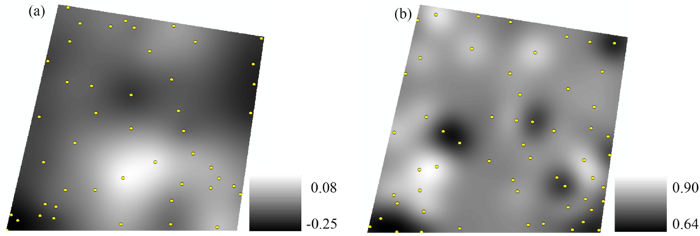
Next, the NDVIs and MSAVIs values of the gv_0 sample locations, and the NDVIv, and MSAVIv values of the fv_1 sample locations were used to predict the values at all other locations by spatial interpolation. The first spatial interpolation method tested was IDW, a deterministic interpolation method that assigns nearer samples greater weight for predictions, and the IDW exponent value controls this weight [35]. A full explanation of IDW is not given in this paper due to its wide availability from other sources, so readers interested in more details are encouraged to refer to [36] or other works in the literature that discuss IDW. IDW is a relatively simple interpolation method, but one advantage is that it requires little parameter calibration, making it fast to implement and quite objective. Many IDW exponent values between 1.0 and 3.0 were tested, and the optimal NDVIs, MSAVIs, NDVIv, and MSAVIv values were optimized through cross-validation of the sample data. As an example, maps of predicted NDVIs and NDVIv (i.e., IDW-NDVIs and IDW-NDVIv) are shown in Figure 3.
The second interpolation method tested was OK, a geostatistical interpolation technique that, unlike IDW, assesses the correlation between sample points to predict the values at all other locations. Along with IDW, OK is one of the most widely-used interpolation methods in the Environmental Sciences [37]. Again, a full explanation of OK is not provided in this paper due to its wide availability from other sources, so readers are referred to [38] and other similar works in the literature for further details. OK model parameters (nugget, partial sill, range, lag size, and number of lags) were optimized by cross-validation of the sample data to limit the potential subjectivity in their selection. As an example, maps of predicted OK-NDVIs and OK-NDVIv are shown in Figure 4. Comparison of the interpolated surfaces in Figures 3 and 4 show that OK interpolation produced a smoother result in general.
3.5. Calculation of FVC Using Invariant and Interpolated VIs and VIv
Next, FVC was calculated for each pixel in the ASTER image using both the traditional VI-based linear mixture method (i.e., with invariant VIs and VIv) and the proposed methods. For the traditional FVC calculation using NDVI, NDVIs in equation 1 was set as the mean (−0.16) of the gv_0 samples and NDVIv was set as the mean (0.77) of the gv_1 samples. For the traditional FVC calculation using MSAVI, MSAVIs was set as the mean (−0.14) of the gv_0 samples and MSAVIv as the mean (0.49) of the gv_1 samples. For the proposed approach, the interpolated NDVI and MSAVI values replaced the invariant values. For all calculations, FVC was constrained to the physically possible 0–1 range by assigning saturated non-vegetated or fully vegetated pixels (i.e., pixels with an estimated FVC < 0 or > 1) a value of 0 or 1, respectively. The number of pixels with FVC < 0 or > 1 was typically between 20 and 30%. For example, when the traditional NDVI approach was used, 11.16% of pixels had FVC < 0 and 18.06% had FVC > 1, while for the OK-NDVI approach, a similar percentage of pixels had FVC < 0 (11.24%) and fewer pixels had FVC > 1 (15.53%).
Compared with the NDVIs values calculated in other FVC studies, which were typically between 0.05–0.20 [11], the mean NDVIs in our study area was lower. This was most likely due to fact that some of the sample non-vegetation pixels in the image contained some frost or snow (which typically has negative NDVI values). We tried to avoid using endmember pixels that contained snow, but this could not be totally avoided because the GeoEye-1 image was taken before the ASTER image (it may have snowed in some areas after the GeoEye-1 image was taken), and it was not always clear in the ASTER image whether or not a pixel was at least partially covered by snow. On the other hand, our mean NDVIv was similar to the NDVIv values of the past studies, also provided in [11]. We did not compare our MSAVIs and MSAVIv values with those of past studies because we could not find reported values.
3.6. Validation of ASTER FVC Estimates
The high resolution GeoEye-1 imagery was used to create a reference dataset for assessing the accuracy of the ASTER FVC estimates. 100 pixels in the ASTER image were randomly selected as validation pixels using a stratified random sampling approach (stratified by FVC’s calculated using the invariant calculation method). This sampling scheme ensured that pixels with varying degrees of FVC were included in the validation dataset. Like [10], we used a 3 × 3 pixel (45 m × 45 m) window at each validation pixel location to reduce the effects of coregistration errors between the ASTER and GeoEye-1 images. For the reference FVC measurements, we overlaid the 45 m × 45 m window at each validation sample location onto the GoeEye-1 imagery, manually delineated all green vegetation within the window, and calculated the vegetation fraction. For the ASTER FVC estimates, the mean FVC of the pixels within the 45 m × 45 m window at each validation location was calculated. Accuracy was assessed by comparing the estimated and reference FVC at each location. To quantify the accuracy of the FVC estimation methods, mean absolute error (MAE) and root mean square error (RMSE) were calculated. The calculations for each are as follows:
where N is the number of samples (100), pi is the predicted FVC of sample k, and oi is the reference FVC. MAE provides the expected FVC error per pixel in the image, while RMSE provides an estimate in which greater weight is given to large errors. In addition to performing accuracy assessment for the validation dataset as a whole, we also subdivided the validation data into “edge pixels” and “non-edge pixels” and assessed the accuracy of each separately to obtain a broader picture of the spatial distribution of errors. A validation pixel was considered to be an edge pixel if the 3 × 3 window it was found within contained a clear boundary between sparsely- and heavily-vegetated land cover. Non-edge pixels were all other pixels in the image, and were typically surrounded by other pixels with relatively-similar spectral characteristics (and thus relatively-similar FVC).
4. Results and Discussion
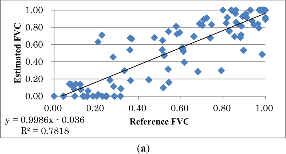
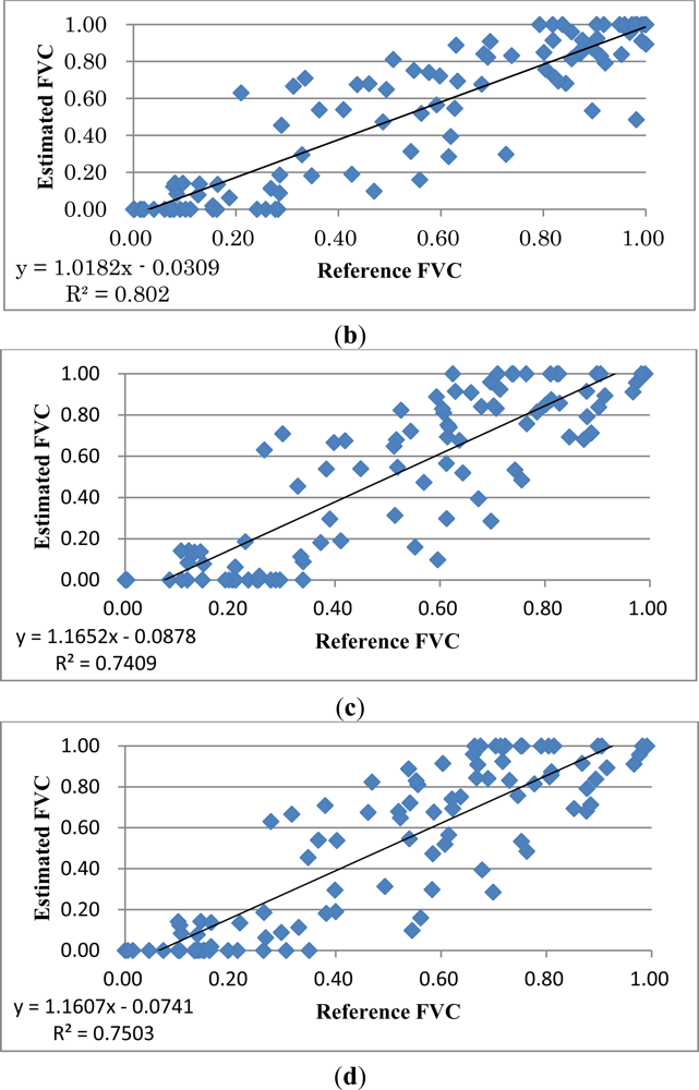
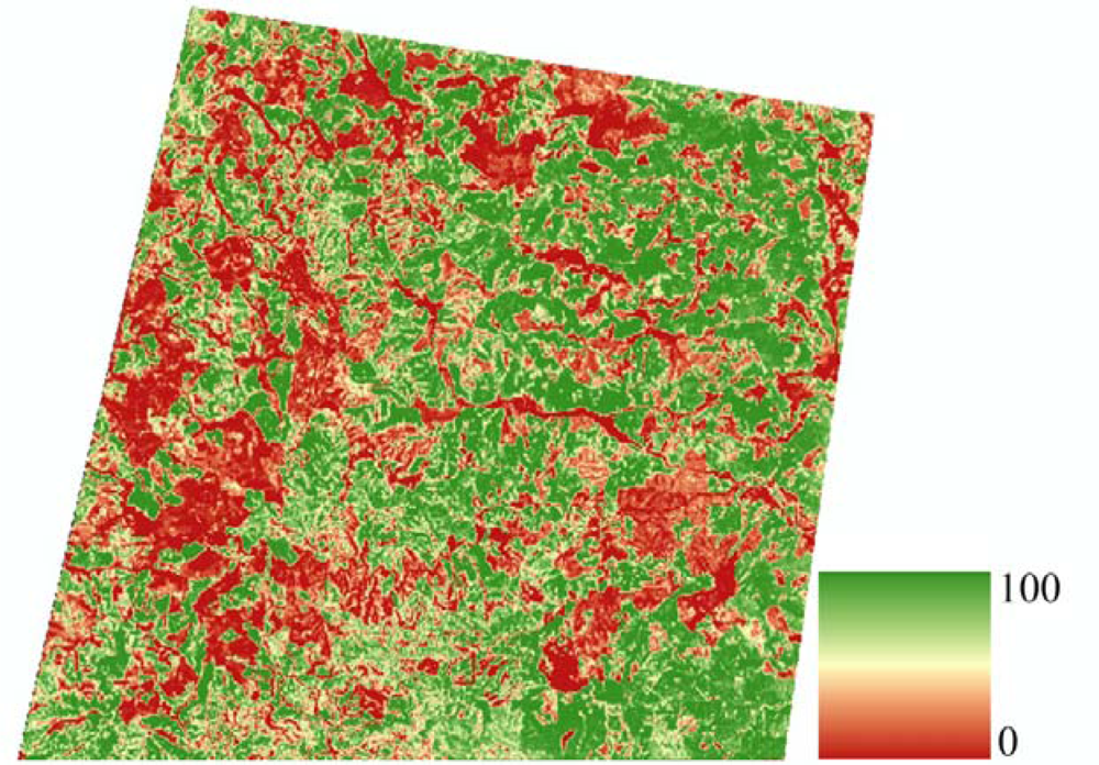
The accuracy of FVC estimates using the traditional method and the proposed spatially interpolated methods are shown in Table 2 for the full validation dataset. The table shows that, when NDVI was used for FVC estimation, OK interpolation reduced MAE from 0.136 to 0.129 (a relative reduction of 5.4%) and RMSE from 0.182 to 0.177 (a relative reduction of 3.8%). IDW interpolation also resulted in a reduction of MAE and RMSE, but by a smaller amount. When MSAVI was used for FVC estimation, OK interpolation reduced MAE from 0.164 to 0.160 (a relative improvement of 2.5%) and RMSE from 0.200 to 0.196 (a relative improvement of 2%), while IDW interpolation led to no reduction in MAE and actually resulted in an increase in RMSE compared to the traditional method. From these results, it is clear that: (i) spatial interpolation of VIs and VIv typically led to a modest reduction in MAE and RMSE, (ii) NDVI estimates of FVC were more accurate than MSAVI estimates, (iii) the improvement in FVC estimates due to spatial interpolation of NDVIs and NDVIv was greater than the improvement due to interpolation of MSAVIs and MSAVIv, and (iv) OK interpolation lead to a greater reduction in MAE and RMSE than IDW interpolation. The overall better performance of OK over IDW in this study is consistent with results from past studies [37], while the better performance of NDVI over MSAVI for FVC estimation, even for the traditional invariant FVC calculation method, was somewhat unexpected due to MSAVI’s intended design to be less sensitive to differences in soil brightness than NDVI. The lower accuracy of MSAVI estimates may have been due to a more non-linear relationship between MSAVI and FVC in our study area, but this could not be confirmed since we did not test non-linear estimation methods. To allow for a visual inspection of results, scatterplots of reference and estimated FVC using the traditional and proposed methods are shown in Figure 5, and the map of FVC produced by the most accurate estimation method, OK-NDVI, is shown in Figure 6.
Table 3 shows the accuracy of FVC estimates for edge (n=43) and non-edge (n=57) validation pixels separately. From this table, it is clear that the accuracy of FVC estimates for edge pixels was considerably lower than that of non-edge pixels, especially for the NDVI calculations. For example, the MAE and RMSE for the most accurate FVC estimation method (OK-NDVI) were 0.175 and 0.219, respectively, for edge pixels, while for non-edge pixels they were 0.095 and 0.136. From Table 3 it is also clear that spatial interpolation increased the accuracy of FVC estimates for both edge and non-edge pixels, but the increase in accuracy was much greater for non-edge pixels. For example, OK-NDVI reduced MAE and RMSE only slightly for edge pixels (a relative reduction of 1.7% and 2.3%, respectively), while the relative reduction in MAE and RMSE for non-edge pixels was much greater (8.7% and 6.2%, respectively).
The lower accuracy of FVC estimates for edge pixels was likely due to two main factors. The first factor was coregistration errors between the low and high resolution images, which were still noticeable even with a registration error of less than 1 pixel and using a 3 × 3 pixel window. These location errors could not be totally avoided since it is practically impossible to achieve a 100% image-to-image registration accuracy [2] and because the window approach is of limited use in patchy environments [39] such as the one in this study area. Even if field measurements of FVC, such as hemispherical photographs [7], are used for validation purposes in place of high resolution imagery, it is still difficult to accurately link field measurements to individual pixels [39]. When a validation pixel was located within a spectrally homogeneous area, the effects of coregistration errors were less significant. The second factor that led to lower accuracy for edge pixels was diffuse reflection from nearby surfaces, which affected the spectral characteristics (and thus the VI calculations) of these edge pixels. For non-edge pixels, the effects of diffuse reflection from nearby surfaces were not as significant because of the high degree of spectral similarity between the non-edge pixels and their surrounding areas. These two factors which led to lower accuracy in FVC estimates for edge pixels also explain why there was less improvement from spatial interpolation of VIs and VIv for these edge pixels, since spatial interpolation of endmember values will not reduce the effects of coregistration errors nor the effects of diffuse reflection. To our knowledge, no past studies have assessed the accuracy of FVC estimates for edge and non-edge pixels separately. However, since we found a large variation in both (a) the accuracy of FVC estimates for edge and non-edge pixels, and (b) the degree to which errors were reduced by the proposed methods for each of these types of pixels, we recommend that future studies in patchy environments report accuracy for both types of pixels to provide better estimates of (a) the spatial distribution of errors and (b) the degree to which new techniques improve FVC estimates for each type of pixel.
5. Conclusions
In this study, we developed a new fractional green vegetation cover (FVC) estimation approach that uses spatial interpolation to predict spectral variations in bare soil (VIs) and green vegetation (VIv) caused by local differences in soil and vegetation conditions. This approach was used to estimate FVC in an Advanced Spaceborne Thermal Emission and Reflection Radiometer (ASTER) image of a forested area. Inverse Distance Weighting (IDW) and Ordinary Kriving (OK) were tested for spatial interpolation, and both the Normalized Differential Vegetation Index (NDVI) and the Modified Soil Adjusted Vegetation Index (MSAVI) were tested for calculation of FVC using the linear Vegetation Index (VI) model described in [3]. We found that spatial interpolation of VIs and VIv reduced the Mean Absolute Error (MAE) and Root Mean Square Error (RMSE) of FVC estimates by up to 5.1% and 2.7%, respectively, for the validation data set as a whole, and by up to 8.7% and 6.2% for non-edge pixels in the validation data set. Use of NDVI in the VI model and OK for interpolation produced these most accurate FVC estimates. The results of this study indicate that spatial interpolation of endmembers’ spectral properties can improve sub-pixel estimates of land cover.
Since the increase in accuracy of the proposed methods was due to the interpolated VIs and VIv values, incorporating a larger number of endmember pixels for interpolation (ideally using automated endmember extraction algorithms like the pixel purity index [40]) or use of more sophisticated spatial interpolation methods is likely to result in further improvement in FVC estimates. The main limitation of our proposed method is that endmember bare soil and green vegetation pixels must be widely distributed across an image to allow for interpolation (rather than extrapolation) of their spectral characteristics, so it may not be applicable when endmembers can be found only within a small subregion of an image. It should be noted that in this study we only used a linear approach for FVC estimation, which is the most commonly-used approach. In addition to non-linear unmixing methods, regression and machine learning algorithms have also been used for FVC estimation (e.g., [10,13]), so a comparison of the accuracy of the proposed methods with the accuracy achieved using spatially-interpolated values for these other FVC estimation methods should be tested in the future. Especially in study areas where endmembers do not exist or are not widely distributed, regression-based methods may provide a better alternative for estimating FVC since mixed pixels can be used to derive the unmixing formula [10]. Finally, in future studies, spatial interpolation of the spectral properties of endmembers should be tested for images containing a higher number of spectral bands (e.g., hyperspectral images) and using a larger number of endmembers.
Acknowledgments
This research was supported by the Japan Society for the Promotion of Science (JSPS) Postdoctoral Fellowship for Foreign Researchers. Orthorectified ASTER data was provided by the Land Processes Distributed Active Archive Center (LP DAAC) located at the US Geological Survey (USGS) Earth Resources Observation and Science (EROS) Center ( lpdaac.usgs.gov).
References
- Adams, J.; Smith, M.; Johnson, P. Spectral mixture modeling: A new analysis of rock and soil types at the Viking Lander 1 Site. J. Geophys. Res 1986, 91, 8098–8112. [Google Scholar]
- de Asis, A.; Omasa, K.; Oki, K.; Shimizu, Y. Accuracy and applicability of linear spectral unmixing in delineating potential erosion areas in tropical watersheds. Int. J. Remote Sens 2008, 29, 4151–4171. [Google Scholar]
- Gutman, G.; Ignatov, A. The derivation of the green vegetation fraction from NOAA/AVHRR data for use in numerical weather prediction models. Int. J. Remote Sens 1998, 19, 1533–1543. [Google Scholar]
- Zeng, X.; Dickinson, R.E.; Walker, A.; Shaikh, M.; Defries, R.S.; Qi, J. Derivation and evaluation of global 1-km fractional vegetation cover data for land modeling. J. Appl. Meteorol 2000, 39, 826–839. [Google Scholar]
- Montandon, L.; Small, E. The impact of soil reflectance on the quantification of the green vegetation fraction from NDVI. Remote Sens. Environ 2008, 112, 1835–1845. [Google Scholar]
- James, K.; Stensrud, D.; Yussouf, N. Value of real-time vegetation fraction to forecasts of severe convection in high-resolution models. Weather Forecast 2009, 24, 187–210. [Google Scholar]
- Jiménez-Muñoz, J.; Sobrino, J.; Plaza, A.; Guanter, L.; Moreno, J.; Martinez, P. Comparison between fractional vegetation cover retrievals from vegetation indices and spectral mixture analysis: Case study of PROBA/CHRIS data over an agricultural area. Sensors 2009, 9, 768–793. [Google Scholar]
- Gilalabert, M.; Gonzalez-Piqueras, F.; Garcia-Haro, F.; Melia, J. A generalized soil-adjusted vegetation index. Remote Sens. Environ 2002, 82, 303–310. [Google Scholar]
- Gitelson, A.; Kaufman, Y.; Stark, R.; Rundquist, D. Novel algorithms for remote estimation of vegetation fraction. Remote Sens. Environ 2002, 80, 76–87. [Google Scholar]
- Xiao, J.; Moody, A. A comparison of methods for estimating fractional green vegetation cover within a desert-to-upland transition zone in central New Mexico, USA. Remote Sens. Environ 2005, 98, 237–250. [Google Scholar]
- Zhou, X.; Guan, H.; Xie, H.; Wilson, J. Analysis and optimization of NDVI definitions and areal fraction models in remote sensing of vegetation. Int. J. Remote Sens 2009, 30, 721–751. [Google Scholar]
- Qi, J.; Marsett, R.; Moran, M.; Goodrich, D.; Heilman, P.; Kerr, Y.; Dedieu, G. Spatial and temporal dynamics of vegetation in the San Pedro River basin area. Agr. For. Meteorol 2000, 105, 55–68. [Google Scholar]
- Guilfoyle, K.; Althouse, M.; Chang, C. A quantitative and comparative analysis of linear and nonlinear spectral mixture models using radial basis function neural networks. IEEE Trans. Geosci. Remote Sens 2001, 39, 2314–2318. [Google Scholar]
- Naksuntorn, N. Nonlinear spectral mixture analysis for hyperspectral imagery in an unknown environment. IEEE Geosci. Remote Sens. Lett 2010, 7, 836–840. [Google Scholar]
- Heylen, R.; Burazerovic, D.; Scheunders, P. Non-linear spectral unmixing by geodesic simplex volume maximization. IEEE J. Sel. Top. Signal Process 2011, 5, 534–542. [Google Scholar]
- Obata, K.; Yoshioka, H. Relationships between errors propogated in fraction of vegetation cover by algorithms based on a two-endmember linear mixture model. Remote Sens 2010, 2, 2680–2699. [Google Scholar]
- Theseira, M.; Thomas, G.; Sannier, A. An evaluation of spectral mixture modeling applied to a semi-arid environment. Int. J. Remote Sens 2002, 23, 687–700. [Google Scholar]
- Obata, K.; Yoshioka, H. Inter-algorithm relationships for the estimation of the fraction of vegetation cover based on a two endmember linear mixture model with the VI constraint. Remote Sens 2010, 2, 1680–1701. [Google Scholar]
- Merlin, O.; Duchemin, B.; Hagolle, O.; Jacob, F.; Coudert, B.; Chehbouni, G.; Dedieu, G.; Garatuza, J.; Kerr, Y. Disaggregation of MODIS surface temperature over an agricultural area using a time series of Formosat-2 images. Remote Sens. Environ 2010, 114, 2500–2512. [Google Scholar] [Green Version]
- Baumgardner, M.; Silva, L.; Biehl, L.; Stoner, E. Reflectance Properties of Soils. In Advances in Agronomy; Brady, N., Ed.; America Press Inc.: Orlando, FL, USA, 1985. [Google Scholar]
- Jensen, J. Introductory Digital Image Processing: A Remote Sensing Perspective, 3rd ed.; Pearson Prentice Hall: Upper Saddle River, NJ, USA, 2004. [Google Scholar]
- Richter, R.; Kellenberger, T.; Kaufmann, H. Comparison of topographic correction methods. Remote Sens 2009, 1, 184–196. [Google Scholar]
- Huete, A. A soil-adjusted vegetation index (SAVI). Remote Sens. Environ 1988, 25, 295–309. [Google Scholar]
- Matsui, T.; Lakshmi, V.; Small, E. The effects of satellite-derived vegetation cover variability on simulated land-atmosphere interactions in the NAMS. J. Climate 2005, 18, 21–40. [Google Scholar]
- Johnson, B.; Tateishi, R.; Xie, Z. Using geographically weighted variables for image classification. Remote Sens. Lett 2012, 3, 491–499. [Google Scholar]
- Rouse, J.; W.; Haas, R.; Schell, J.; Deering, D.; Harlan, J. Monitoring the Vernal Advancement of Retrogradation of Natural Vegetation; Type III Final Report; NASA/GSFC: Greenbelt, MD, USA, 1974; p. 371. [Google Scholar]
- Qi, J.; Chehbouni, A.; Huete, A.; Kerr, Y.; Sorooshian, S. A modified soil adjusted vegetation index (MSAVI). Remote Sens. Environ 1994, 48, 119–126. [Google Scholar]
- Kodani, J. Ecology and management of conifer plantations in Japan: control of tree growth and maintenance of biodiversity. J. Forest Res 2006, 11, 267–274. [Google Scholar]
- Seiwa, K.; Eto, Y.; Masaka, K. Effects of thinning intensity on species diversity and timber production in a conifer (Cryptomeria japonica) plantation in Japan. J. Forest. Res 2011. [Google Scholar] [CrossRef]
- Japan Ministry of Agriculture, Forestry and Fisheries. Annual Report on Forest and Forestry in Japan: Fiscal Year 2010 (Summary). 2010. Available online: http://www.rinya.maff.go.jp/j/kikaku/hakusyo/22hakusho/pdf/22_e.pdf (accessed on 20 June 2012).
- Smith, M.; Milton, E. The use of the empirical line method to calibrate remotely sensed data to reflectance. Int. J. Remote Sens 1999, 20, 2653–2662. [Google Scholar]
- Chavez, P. Image-based atmospheric corrections—Revisited and improved. Photogramm. Eng. Remote Sensing 1996, 62, 1025–1036. [Google Scholar]
- Baldridge, A.; Hook, S.; Grove, C.; Rivera, G. The ASTER Spectral Library Version 2.0. Remote Sens. Environ 2009, 113, 711–715. [Google Scholar]
- Moran, P. Notes on continuous stochastic phenomena. Biometrika 1950, 37, 17–23. [Google Scholar]
- Lam, N. Spatial interpolation methods: A review. Cartogr. Geogr. Inform 1983, 10, 129–150. [Google Scholar]
- O’Sullivan, D.; Unwin, D. Geographic Information Analysis; John Wiley & Sons, Inc: Hoboken, NJ, USA, 2003. [Google Scholar]
- Li, J.; Heap, A. A review of comparative studies of spatial interpolation methods in environmental sciences: Performance and impact factors. Ecol. Inform 2011, 6, 228–241. [Google Scholar]
- Kleijnen, J. Kriging metamodeling in simulation: A review. Eur. J. Oper. Res 2009, 192, 707–716. [Google Scholar]
- Kuemmerle, T.; Roder, A.; Hill, J. Separating grassland and shrub vegetation by multidate pixel-adaptive spectral mixture analysis. Int. J. Remote Sens 2006, 27, 3251–3271. [Google Scholar]
- Boardman, J. Geometric Mixture Analysis of Imaging Spectrometry Data. Proceedings of International Geoscience and Remote Sensing Symposium, Pasadena, CA, USA, 8–12 August 1994; 4, pp. 2369–2371.
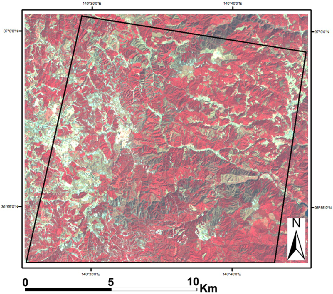
Figure 1.
False color Advanced Spaceborne Thermal Emission and Reflection Radiometer (ASTER) image, with the study area outlined in black (centered at 36°57′N, 140°38′E). NIR, R, and Green ASTER bands are shown in red, green, and blue color, respectively.
Figure 1.
False color Advanced Spaceborne Thermal Emission and Reflection Radiometer (ASTER) image, with the study area outlined in black (centered at 36°57′N, 140°38′E). NIR, R, and Green ASTER bands are shown in red, green, and blue color, respectively.

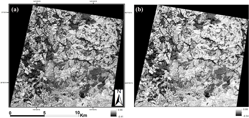
Figure 2.
Normalized Differential Vegetation Index (NDVI) (a) and Modified Soil Adjusted Vegetation Index (MSAVI) (b) images of the study area. The topographic effects evident in Figure 1 have been largely removed using the vegetation indices.
Figure 2.
Normalized Differential Vegetation Index (NDVI) (a) and Modified Soil Adjusted Vegetation Index (MSAVI) (b) images of the study area. The topographic effects evident in Figure 1 have been largely removed using the vegetation indices.

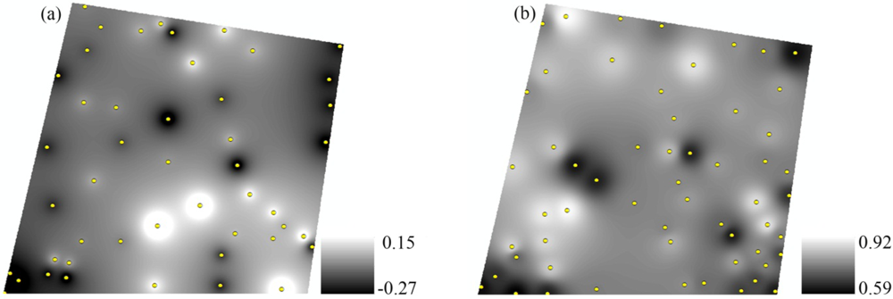
Figure 3.
Predicted NDVIs (a) and NDVIv (b) values using Inverse Distance Weighting (IDW) interpolation. Yellow points show the locations of gv_0 (a) and gv_1 (b) samples. Optimal IDW exponent value was 1.12 for (a) and 2.45 for (b).
Figure 3.
Predicted NDVIs (a) and NDVIv (b) values using Inverse Distance Weighting (IDW) interpolation. Yellow points show the locations of gv_0 (a) and gv_1 (b) samples. Optimal IDW exponent value was 1.12 for (a) and 2.45 for (b).

Figure 4.
Predicted NDVIs (a) and NDVIv (b) values using Ordinary Kriging (OK) interpolation. Yellow points show the locations of gv_0 (a) and gv_1 (b) samples.
Figure 4.
Predicted NDVIs (a) and NDVIv (b) values using Ordinary Kriging (OK) interpolation. Yellow points show the locations of gv_0 (a) and gv_1 (b) samples.

Figure 5.
Scatterplots of Reference and Estimated FVC using the NDVI (a), OK-NDVI (b), MSAVI (c), and OK-MSAVI (d) approach. OK-NDVI and OK-MSAVI show a modestly better linear fit than NDVI and MSAVI (based on R2 values).
Figure 5.
Scatterplots of Reference and Estimated FVC using the NDVI (a), OK-NDVI (b), MSAVI (c), and OK-MSAVI (d) approach. OK-NDVI and OK-MSAVI show a modestly better linear fit than NDVI and MSAVI (based on R2 values).


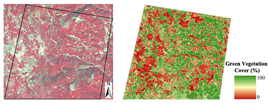
Figure 6.
Estimated FVC (%) using the most accurate estimation method, OK-NDVI.


Table 1.
Moran’s I (MI) and p values for NDVIs, NDVIv, MSAVIs, and MSAVIv. All endmembers exhibit positive spatial autocorrelation.
| NDVI | MSAVI | |||
|---|---|---|---|---|
| MI | p | MI | p | |
| Vis | 0.23 | 0.03 | 0.30 | 0.004 |
| VIv | 0.15 | 0.07 | 0.10 | 0.20 |
Table 2.
Mean absolute error (MAE) and root mean square error (RMSE) for each FVC estimation method. For the proposed spatially interpolated estimation methods, relative changes in MAE and RMSE (%) show the changes compared to the invariant FVC calculation method.
| FVC Estimation Method | MAE | Relative Change in MAE (%) | RMSE | Relative Change in RMSE (%) |
|---|---|---|---|---|
| NDVI (invariant) | 0.136 | 0.182 | ||
| OK-NDVI | 0.129 | −5.1% | 0.177 | −2.7% |
| IDW-NDVI | 0.131 | −3.7% | 0.179 | −1.6% |
| MSAVI (invariant) | 0.164 | 0.200 | ||
| OK-MSAVI | 0.16 | −2.4% | 0.196 | −2.0% |
| IDW-MSAVI | 0.164 | 0% | 0.202 | +1.0% |
Table 3.
Mean absolute error (MAE), root mean square error (RMSE), and their relative changes in edge and non-edge pixels. Much more improvement in estimation accuracy is seen in non-edge pixels.
| Pixel Type | FVC Estimation Method | MAE | Relative Change in MAE (%) | RMSE | Relative Change in RMSE (%) |
|---|---|---|---|---|---|
| Edge | NDVI | 0.178 | 0.221 | ||
| OK-NDVI | 0.175 | −1.7% | 0.219 | −0.9% | |
| IDW-NDVI | 0.174 | −2.2% | 0.22 | −0.5% | |
| MSAVI | 0.183 | 0.218 | |||
| OK-MSAVI | 0.182 | −0.5% | 0.219 | +0.5% | |
| IDW-MSAVI | 0.186 | +1.6% | 0.226 | +3.6% | |
| Non-edge | NDVI | 0.104 | 0.145 | ||
| OK-NDVI | 0.095 | −8.7% | 0.136 | −6.2% | |
| IDW-NDVI | 0.098 | −5.8% | 0.139 | −4.1% | |
| MSAVI | 0.149 | 0.184 | |||
| OK-MSAVI | 0.144 | −3.4% | 0.178 | −3.3% | |
| IDW-MSAVI | 0.147 | −1.3% | 0.182 | −1.1% | |
Share and Cite
MDPI and ACS Style
Johnson, B.; Tateishi, R.; Kobayashi, T. Remote Sensing of Fractional Green Vegetation Cover Using Spatially-Interpolated Endmembers. Remote Sens. 2012, 4, 2619-2634. https://doi.org/10.3390/rs4092619
AMA Style
Johnson B, Tateishi R, Kobayashi T. Remote Sensing of Fractional Green Vegetation Cover Using Spatially-Interpolated Endmembers. Remote Sensing. 2012; 4(9):2619-2634. https://doi.org/10.3390/rs4092619
Chicago/Turabian StyleJohnson, Brian, Ryutaro Tateishi, and Toshiyuki Kobayashi. 2012. "Remote Sensing of Fractional Green Vegetation Cover Using Spatially-Interpolated Endmembers" Remote Sensing 4, no. 9: 2619-2634. https://doi.org/10.3390/rs4092619