Tree Species Classification with Random Forest Using Very High Spatial Resolution 8-Band WorldView-2 Satellite Data


Institute of Surveying, Remote Sensing and Land Information (IVFL), University of Natural Resources and Life Sciences (BOKU), Peter Jordan Str. 82, A-1190 Vienna, Austria
*
Author to whom correspondence should be addressed.
Remote Sens. 2012, 4(9), 2661-2693; https://doi.org/10.3390/rs4092661
Submission received: 25 July 2012
/
Revised: 3 September 2012
/
Accepted: 4 September 2012
/
Published: 14 September 2012
(This article belongs to the Special Issue Remote Sensing of Biological Diversity)
Abstract
:Tree species diversity is a key parameter to describe forest ecosystems. It is, for example, important for issues such as wildlife habitat modeling and close-to-nature forest management. We examined the suitability of 8-band WorldView-2 satellite data for the identification of 10 tree species in a temperate forest in Austria. We performed a Random Forest (RF) classification (object-based and pixel-based) using spectra of manually delineated sunlit regions of tree crowns. The overall accuracy for classifying 10 tree species was around 82% (8 bands, object-based). The class-specific producer’s accuracies ranged between 33% (European hornbeam) and 94% (European beech) and the user’s accuracies between 57% (European hornbeam) and 92% (Lawson’s cypress). The object-based approach outperformed the pixel-based approach. We could show that the 4 new WorldView-2 bands (Coastal, Yellow, Red Edge, and Near Infrared 2) have only limited impact on classification accuracy if only the 4 main tree species (Norway spruce, Scots pine, European beech, and English oak) are to be separated. However, classification accuracy increased significantly using the full spectral resolution if further tree species were included. Beside the impact on overall classification accuracy, the importance of the spectral bands was evaluated with two measures provided by RF. An in-depth analysis of the RF output was carried out to evaluate the impact of reference data quality and the resulting reliability of final class assignments. Finally, an extensive literature review on tree species classification comprising about 20 studies is presented.
1. Introduction
Tree species diversity is a key parameter to describe forest ecosystems. It is a relevant parameter for various ecological issues such as wildlife habitat modeling and it is also becoming more and more important in sustainable forest management [1–3]. For example, in close-to-nature forest management pure stands are replaced by heterogeneous, mixed stands. Hence, spatially detailed tree species information is of high importance. Traditional forest inventories and other field-based data acquisition methods, such as stand estimation, are not suitable for such tasks. It is nearly impossible to acquire detailed tree species information over large areas purely on the basis of field assessments. Therefore, enhanced methods are required to get spatially-explicit information on the tree species composition and distribution patterns.
Remote sensing is particularly useful for this task, as it provides a synoptic view and delivers information over large areas at a high level of detail [4]. There is a large variety of sensors with a wide range of spatial and spectral resolution. For tree species classification at crown scale in forests with high tree species diversity, data with both high spatial and spectral resolution are desirable (e.g., [4–7]). Airborne cameras provide data with the highest spatial resolution that is available at the moment. However, they are limited to the spectral bands Blue, Green, Red, and Near Infrared. Besides, due to their wide field of view, aerial photos show strong effects caused by the bi-directional reflectance characteristics of most land cover types. Depending on the sun-view-geometry, which varies with the position of the object within the image, the spectral signature of an object can differ significantly. Although these effects can be useful in special image analysis techniques [8], they are usually regarded as a limiting factor in automatized analysis of aerial images. Airborne hyperspectral sensors meet the requirements regarding spectral and spatial resolution. However, due to the high costs and their still limited availability, hyperspectral data have gained only limited acceptance for operational use yet. Satellite-borne multispectral sensors either have a high spatial resolution but provide only the 4 standard bands (Blue, Green, Red, Near Infrared), such as IKONOS or QuickBird, or they provide more bands but only with lower spatial resolution, such as MODIS, Landsat, ASTER, and SPOT.
In 2009, WorldView-2, a new satellite-borne sensor, was launched by DigitalGlobe. The very high spatial resolution (0.5 m in the panchromatic band and 2.0 m in the multispectral bands) and 4 new spectral bands (Coastal, Yellow, Red Edge and Near Infrared 2) additional to the 4 standard bands (Blue, Green, Red, and Near Infrared 1), give reason to expect that this sensor has a high potential for tree species mapping. The data provider postulates that all 4 new bands are strongly related to vegetation properties. For example, the reflectance measured in the Coastal band is related to the chlorophyll content of plants. The Yellow band is intended for the detection of ‘yellowness’ of targets, for example, of tree crowns caused by insect diseases. The Red Edge band is supposed to discriminate between healthy trees and trees that are impacted by disease and to enhance the separation between different species and age classes. The Near Infrared 2 band that partly overlaps the standard Near Infrared 1 band but is less affected by atmospheric influence is expected to enable sophisticated vegetation analysis, such as biomass studies [9].
In some recently published studies on tree species mapping with WorldView-2 data, promising results have been obtained [10–14]. However, studies in European forests are still missing. Therefore, for the present study an area located in Austria was chosen to test the suitability of WorldView-2 for tree species mapping. The area is ideally suited for this purpose, as it is very rich in tree species compared to other European forest biomes, such as boreal forests.
Non-parametric methods are very attractive for classification purposes, as they can be used with arbitrary data distributions and without the assumption that the forms of the underlying densities are known [15]. They are, therefore, applicable to a huge variety of practical classification problems. Random Forest [16] is one of the most recent non-parametric methods. It is a very accurate classifier and robust against noise [16–18]. Compared to other non-parametric methods, the setup of a RF is simple, because no sophisticated parameter tuning is necessary.
In the last decade, RF has become increasingly important in remote sensing. It has been used, for example, to classify land cover [18–22] and ecological zones [23], to identify spectral differences of tree species [24–27], to map landslides [28], to create forest canopy fuel maps for fire forecasting [29], to quantify aboveground forest carbon pools [30], and to analyze urban areas [31]. RF is often employed together with hyperspectral data, which provide a very large number of input variables [21,24–26]. That is because RF is, in contrast to parametric methods, relatively insensitive to the small sample size problem (i.e., the number of training samples per class is significantly smaller than the dimension of the feature space, also called ‘Hughes effect’) [32,33]. Besides, there are studies with multispectral satellite data with medium (Landsat) [21,22] and high spatial resolution (IKONOS, QuickBird) [28]. The RF classifier was also successfully used together with LiDAR (Light Detection and Ranging) data, either in combination with spectral data [25,31] or by itself [30].
When image data is acquired at high spatial resolution, object-based image analysis approaches have proven to be superior to pixel-based approaches. This is true in particular, if the pixel size is significantly smaller than the average size of the objects of interest [34–36]. In our study, the sunlit regions of individual tree crowns are the objects of interest. Depending on the size of the tree and on the crown form (conical, spherical), the size of these regions varies in the 2 m multispectral image from a few (about 2 or 3) to several (about 10 to 20) pixels. As it is not known in advance, if the pixel-based or the object-based approach will perform better in tree species discrimination, a comparison of these two concepts of image analysis is required.
This study aims at separating 10 tree species in a mid-European, submontane forest using spectral information provided by the WorldView-2 sensor applying Random Forest classification. We focus on the following research questions: (1) Which tree species can be separated by WorldView-2 data and which accuracies can be achieved? (2) Do the 4 additional bands of WorldView-2 improve the classification accuracy significantly compared to the 4 standard bands? (3) Is the classifier Random Forest suitable for detailed tree species classification, and (4) which approach performs better, an object-based or a pixel-based one?
2. Material
2.1. Study Site
The study site covers approximately 3000 ha and is located in the East of Austria (47°38′N, 16°26′E) in the province of Burgenland. The terrain is hilly and lies in the submontane life zone with an elevation between 290 and 670 m above sea level. The annual rainfall is between 700 and 1,100 mm, with a maximum in summer. The bedrocks are mainly base-poor silicates, quartz phyllite and gneiss. The potential natural forest community ranges from oak-hornbeam forest over pine-oak forest to fir-beech forest with admixture of oak, chestnut and Scots pine [37]. The privately owned forest is commercially used focusing on timber production and hunting.
As a result of forest management, the area is dominated by Norway spruce (Picea abies, (L) Karst.), Scots pine (Pinus sylvestris, L.), European beech (Fagus sylvatica, L.) and English oak (Quercus robur, L.). Secondary tree species are Silver fir (Abies alba, Mill.), European larch (Larix decidua, Mill.), Douglas fir (Pseudotsuga menziesii, (Mirb.) Franco), Lawson’s cypress (Chamaecyparis lawsoniana, (A. Murr.) Parl.), Grand fir (Abies grandis, Lindl), Ponderosa pine (Pinus ponderosa, Douglas ex P. et C. Laws), European ash (Fraxinus excelsior, L.), European hornbeam (Carpinus betulus, L.), Turkey oak (Quercus cerris, L.), Silver birch (Betula pendula, Roth), European alder (Alnus glutinosa, L.), Persian walnut (Juglans regia, L.), Black locust (Robinia pseudoacacia, L.), European chestnut (Castanea sativa, Mill.), Sweet cherry (Prunus avium, L.), linden- (Tilia sp.), maple- (Acer sp.), elm- (Ulmus sp.) and poplar-species (Populus sp.). The tree species Douglas fir, Lawson’s cypress, Grand fir, Ponderosa pine, and Black locust are allochthonous species in Europe.
2.2. Reference Data
For generating reference data we concentrated on pure and homogeneous stands identified by a forest stand map. A stand map is a common instrument in traditional forest management planning and contains key attributes for each stand, such as timber volume, basal area, age, and tree species composition. The tree species composition is estimated in the field by an evaluator (stand estimation). The procedure is quite fast and gives a good overview for each stand. However, in large and heterogeneous stands the stand description usually does not provide detailed information about the spatial distribution of all occurring tree species. For this reason we used inventory data (angle count sample plots in a regular 200 m grid) as additional information.
The chosen stands were distributed over the whole study site (Figure 1). Within these stands, clearly identifiable tree crowns were selected on the image with 0.5 m pixel size. The selected trees belonged mainly to the middle and old age classes, where the crowns could be easily detected. For each reference tree we delineated the sunlit part of the crown to minimize shadow effects [5,38,39]. The manual delineation was done by setting points on all relevant crown pixels on the 2 m image (Figure 2). Then the points were converted into polygons following the pixel edges. To each tree crown the tree species information specified in the forest stand map or in the inventory data and the spectral information from the WorldView-2 image were assigned. For the object-based approach, we calculated the mean band values for each crown polygon using its within-crown pixel spectra. For the pixel-based approach, we used the individual pixel spectra.
We included the 4 main tree species Norway spruce, Scots pine, European beech and English oak and 6 secondary tree species in the analysis. For the other tree species listed in Section 2.1 we could not identify a sufficient number of individual tree crowns. Table 1 shows the tree species included in the study as well as the number of pixels and objects (tree crowns) per tree species. In total, 1,465 reference polygons were delineated. In the sample, the distribution by tree species corresponds roughly to the distribution in the study site. In addition to classification of the 10 tree species we included also the classification with only 4 (main) species (PA, PS, FS and QR) for comparability with studies that comprise only a few tree species, e.g. studies in boreal forests.
2.3. Test Area
For plausibility checks and for demonstrating the method on a continuous area, we selected a test area covered by an approximately 50 years old mixed forest characterized by a high tree species diversity (yellow area in Figure 1). The test area represents an independent data set as it does not contain any reference trees used for building the classifiers (Section 3.3). For the whole test area all visible tree crowns were delineated as described in Section 2.2 and illustrated in Figure 2. To assess classification results for this area, forest management data was consulted. However, as explained in Section 2.2 this data provides only rough information on the true tree species composition. Therefore, the classification results were also verified in the field.
2.4. WorldView-2 Image
The WorldView-2 image was recorded under cloudless conditions over the site in the middle of the growing season on 10 July 2010 (Processing Level: Ortho Ready Standard, Scan Direction: forward, Mean Satellite Elevation: 77.8°, Mean Satellite Azimuth: 76.6°, and Mean Off Nadir View Angle: 11°). At this time of the year, the leaves of all tree species are fully developed, which provides good conditions for tree species classification. The WorldView-2 satellite provides high spatial resolution data with 8 spectral bands. At nadir the ground resolution (GSD) is 50 cm for the panchromatic band (0.46–0.80 μm) and 200 cm for the multispectral bands. In addition to the 4 standard bands Blue (0.45–0.51 μm), Green (0.51–0.58 μm), Red (0.63–0.69 μm), and Near Infrared 1 (0.77–0.90 μm), another 4 bands are available. The new bands are Coastal (0.40–0.45 μm), Yellow (0.59–0.63 μm), Red Edge (0.71–0.75 μm), and Near Infrared 2 (0.86–1.04 μm). Further details about the sensor can be found on the website of the provider ( http://worldview2.digitalglobe.com/) and in [40]. WorldView-2 data can be ordered either with the 4 standard bands or with all 8 bands.
The pixel gray values (digital numbers) were converted to ‘at-sensor’ radiance [40]. In addition, we performed an atmospheric correction with the ENVI module (ENVI 4.8) FLAASH resulting in top-of-canopy reflectance. This step was done to derive meaningful spectral reflectance signatures of the tree species. The settings were chosen iteratively by checking the resulting reflectance values for plausibility (final FLAASH settings: Atmospheric Model: Mid-Latitude Summer, Aerosol Model: Rural, Initial Visibility: 70 km). For pansharpening, the HCS algorithm (Hyperspherical Color Space algorithm) [41] was used. This algorithm is dedicated to WorldView-2 data and is implemented in ERDAS Imagine 2010. With ERDAS Imagine the image was georectified by using a digital terrain model (5 m grid). The coordinates of the control point were taken from a color-infrared orthophoto (recorded in 2007, 0.5 m pixel size). The achieved average accuracy (RMSE) was 0.70 pixels on the 2 m image.
3. Methods
For tree species classification we applied object-based and pixel-based approaches using manually delineated sunlit regions of the tree crowns (Section 2.2). As input features, either the spectral information of the 8 WorldView-2 bands were used or only the 4 standard bands.
3.1. Spectral Variability Within and Among Tree Species
Figure 3 shows the mean spectral signatures for the 10 tree species. As expected, the reflectance values in the Red Edge band and in the two Near Infrared bands are higher for the broadleaf tree species than for the conifers [42–44]. European beech (FS) and European hornbeam (CP) show the highest values and differ significantly from the other tree species, whereas the differences between the other broadleaf tree species are much lower (Figure 3(a)). Among the conifers the Lawson’s cypress (CL) shows the highest reflectance values in the near infrared, followed by Douglas fir (PM), European larch (LD), Scots pine (PS) and Norway spruce (PA). In the visible (Figure 3(b)) the bands Green and Yellow show the largest differences, but the differentiation is not as clear as in the near infrared.
The box-whisker-plots in Figure 4 show the spectral variability among and within the 10 tree species. The conifers and the broadleaf trees are well distinguishable by the bands in the near infrared. Within these tree species groups the separation is not so clear. Partly, there are considerable spectral overlaps. Some tree species differ clearly from the other species in particular bands, for example Scots pine (PS) in the bands Coastal and Blue, Silver birch (BP) in the band Yellow, and European beech (FS) in the bands Near Infrared 1 and Near Infrared 2. The tree species show band-specific within-species variance. For example for European hornbeam (CB) the variance in the Red band is quite large compared to the other broadleaf trees and that in the Coastal band is relatively small.
3.2. Band Correlations
On the basis of the correlation matrix computed from the reference samples (Table 2), we could identify 3 groups of bands: (A) Coastal, Blue, (Red), (B) Green, Yellow, (Red), and (C) Red Edge, Near Infrared 1, and Near Infrared 2. Within each group the correlations between the bands are high. The Red band is put in brackets, because it shows high correlation with Blue (Group A) as well as with Green and Yellow (Group B). Each group contains 1 or 2 bands from the 4 standard bands and from the 4 new bands respectively. Thus, the standard bands and the new bands are partly highly correlated providing redundant information.
3.3. Random Forest and Linear Discriminant Analysis
For classification we used Random Forest (RF) [16], a non-parametric ‘ensemble learning’ algorithm. It is an enhancement of traditional decision trees and consists of a large number of trees. For the construction of each decision tree an individual bootstrap sample is drawn from the original data set (sampling with replacement). The split determination at each node is based on the Gini criterion. In standard decision trees, the nodes are split by the variable that gives the best split, i.e., the highest decrease in Gini. In RF, a subset of variables is randomly selected at each node, and from this subset the best-splitting variable is chosen. New data are classified by taking the majority vote among the classification outcomes of all constructed decision trees. For estimating the classification error, the samples not in the bootstrap sample (out-of-bag data, OOB), approximately 36.8% of the original data set at each bootstrap iteration, are used. Each decision tree is used to classify the samples in the corresponding OOB data set. Then for each sample in the original data set the majority vote among the classification outcomes of the involved decision trees is compared with the true class label giving an estimate of the misclassification rate.
RF provides two measures to assess the explanatory power of the input variables, i.e., mean decrease in accuracy (MDA) and mean decrease in Gini (MDG). To calculate the MDA of a variable, the values of this variable are randomly permuted for the OOB data, while keeping the values of the other variables constant. The importance of the variable is obtained by comparing the resulting misclassification rate with the rate achieved without randomly permuting the values of the variable. This procedure is repeated for each variable [16]. To calculate the MDG of a variable, the decreases in the splitting criterion Gini related to this variable are summarized in the forest and normalized by the number of trees [45]. A detailed description of RF can be found in [16,17] and in particular for remote sensing applications in [18,22].
To run a RF classifier, two parameters have to be set: the number of classification trees (number of bootstrap iterations) and the number of input variables used at each node. We varied both parameters across a wide range of values (number of trees: 1 to 2,500; number of random split variables at each node: 1 to 5). The overall accuracy (object-based, 10 tree species, 8 bands) averaged over 20 repetitions increased sharply until reaching a plateau of 250 trees with accuracies remaining almost constant beyond this point (Figure 5). Using 1 or 2 randomly selected input variables per node delivered better results than using 3, 4 or 5 variables. For this reason and for comparability with other studies, we chose the default settings of 500 trees and 2 (the square root of the number of input variables) variables at each node [17,46].
For comparison, we applied also Linear Discriminant Analysis (LDA), which is an established and widely used parametric statistical classifier that is also used in remote sensing [5,47–52]. It estimates linear decision boundaries to separate the classes. As a prerequisite, the classes should be approximately Gaussian distributed and should have equal covariance [17]. The classification accuracies were determined by bootstrapping [53] with 500 bootstrap iterations. The test-datasets of all iterations were identical with the respective RF OOB datasets.
To evaluate the results of RF and LDA we produced confusion matrices with the majority vote from all bootstrap iterations and calculated the producer’s and user’s accuracies for each class, the overall accuracy (correct classification rate), and Cohen’s Kappa coefficient [54]. For the comparison of different methods we used Kappa and its variance to implement Z-Statistic [55].
3.4. Explanatory Power of the Spectral Bands
For a better understanding of the whole classification process we wanted to figure out, which input variables (bands) are most relevant for tree species classification and particularly to investigate the role of the 4 new WorldView-2 bands Coastal, Yellow, Red Edge, and Near Infrared 2.
Both RF and LDA provide measures for assessing variable importance. In RF we used the measures MDA and MDG (Section 3.3). In addition we computed Wilks’ Lambda that is a product of the ANOVA performed prior to LDA and measures the univariate separation power of the variables. In the LDA the multivariate explanatory power of the variables was obtained from the mean discriminant function coefficients (MDFC). For this measure the coefficients of the discriminant functions are standardized and their weighted averages over the discriminant functions are computed [56]. In addition to these measures we determined the overall accuracy for all possible combinations with 4 bands (in total 70 combinations) both with RF (averaged over 20 repetitions) and LDA (with all samples), and identified the 4-band combination that gave the highest classification accuracy. Then we compared the best classification result of RF and LDA, respectively, with the results achieved with the 4-band combinations proposed by MDA, MDG, MDFC, and Wilks’ Lambda.
3.5. Classification Stability
The Random Forest classifier is an ensemble method that combines several individual classification trees (e.g., 500) and is therefore able to adjust for the instabilities of the individual classification trees. Each classification tree outputs a class and the class that is the majority vote is assigned to the instance to be classified (Section 3.3). Hence, in addition to the final class decision, i.e., the majority vote, the class distribution among the votes of all trees is also known. It shows how ambiguous the decision is and which classes are involved. By examining this information, further insights can be gained both in the context of validation and of prediction.
In the validation phase, the number of votes for the most frequent class divided by the number of times the sample appears in the out-of-bag (OOB) dataset serves as a measure of ambiguity:
| UV | Unambiguity for a reference sample (validation); |
| Nmajority | Number of votes for the most frequent class; |
| NOOB | Number of times the sample appears in the out-of-bag (OOB) dataset. |
Three cases of validation outcome can be distinguished (Table 3). We computed the unambiguity for each reference sample and from this we derived for each case (a, b, and c) and for each tree species the distribution of unambiguity. This information can, for example, be used for locating outliers in the reference dataset. Samples that are misclassified with a high unambiguity (case b or c) are outlier candidates and should be verified.
In the prediction phase, the unambiguity of a new sample is computed by dividing the number of votes for the most frequent class by the number of trees in the RF model (Equation (2)) as each new sample is classified by all classification trees of the RF model.
| UP | Unambiguity for a new sample (prediction); |
| Nmajority | Number of votes for the most frequent class; |
| Ntrees | Number of trees in the RF model. |
In combination with the ordinary class-specific user’s accuracies derived in the validation phase, the unambiguity gives an estimate of the achieved classification reliability for each new sample to be classified:
| RP | Reliability for a new sample (prediction); |
| UP | Unambiguity for a new sample (prediction); |
| UAcc | User’s accuracy of the most frequent class. |
In addition, the retrieved classification ambiguities computed for new samples offer the possibility to compute the class-specific probabilities for each sample to be classified, enabling a soft classification (not implemented in the paper).
4. Results
4.1. Object-Based Classification Results for 4 Tree Species
Table 4 shows the results for the object-based classification of the 4 main tree species using all 8 bands of the WorldView-2 image. All user’s and producer’s accuracies were over 90% without any misclassifications between coniferous and broadleaf tree species. From the 860 samples only 36 were misclassified, resulting in an overall accuracy of 95.9% (Kappa 0.945).
If only the 4 standard bands instead of the 8 bands were used, the results degraded only slightly (not shown). The user’s and producer’s accuracies of the individual trees species and also the overall accuracy with 95.5% (Kappa 0.939) were almost the same as the results achieved with all 8 bands. This shows that the new WorldView-2 bands have no positive influence on classifying only a small number of tree species.
4.2. Object-Based Classification Results for 10 Tree Species
The confusion matrix in Table 5 summarizes the results for classifying 10 tree species using all 8 bands. The overall accuracy was 82.4%, 81.2% of the conifers and 83.8% of the broadleaf trees were classified correctly. The separation into coniferous and broadleaf trees (computed after post-classification grouping) was achieved with an overall accuracy of 99.2%.
Large differences between the 10 tree species were observed. The producer’s accuracies ranged from 33.3% (European hornbeam, CB) to 94.3% (European beech, FS), and the user’s accuracies from 57.4% (European hornbeam, CB) to 92.1% (Lawson’s cypress, CL). The European larch (LD) shows with 66.4% the lowest producer’s accuracy and with 70.4% also the lowest user’s accuracy among the conifers. Among the broadleaf tree species, the European hornbeam (CB) shows the lowest accuracies. The best agreements were obtained for European beech (FS), Silver birch (BP), Scots pine (PS) and Lawson’s cypress (CL).
If only the 4 standard bands instead of the 8 bands were used for the differentiation of the 10 tree species, the classification accuracy decreased. Table 6 shows that the producer’s and user’s accuracies for all tree species (except English oak, QR) were significantly lower than the corresponding values achieved with 8 bands (Table 5). The overall accuracy was reduced by 4.9 percentage points.
4.3. Pixel-Based Classification Results for 10 Tree Species
The results of the pixel-based classification are presented in Table 7 (10 tree species, 8 bands). Comparing the results with the corresponding results of the object-based classification (Table 5) revealed that the results of the pixel-based approach were significantly worse than those of the object-based approach. This finding was evident for all tree species included in the study, except two tree species. For English oak (QR) the producer’s accuracy was slightly higher and for European hornbeam (CB) the user’s accuracy did not change.
4.4. Summary of RF Classification Results and Comparison with LDA
The tree specific classification results (user’s accuracies) are summarized in Figure 6 (RF, 10 tree species). Figure 6(a) shows the effect of using the full spectral resolution (i.e., 8 bands) in relation to the sole use of the 4 standard bands. Only three tree species (European larch (LD), Douglas fir (PM), and European Hornbeam (CB)) benefited from the additional bands significantly with an increase in user’s accuracies between 8 and 15 percentage points, i.e., the tree species that had the lowest user’s accuracies using only 4 bands. For the remaining tree species the improvements were moderate (ranging between 1 and 6 percentage points).
By classifying objects instead of pixels the user’s accuracies could be raised significantly for most tree species (Figure 6(b)). Only for European Hornbeam (CB) no improvements could be found. In general, the positive impact was higher for conifers, ranging between 9 and 22 percentage points, than for broadleaf trees, ranging between 4 and 10 percentage points.
Comparing the two charts, it is remarkable that the positive impact of the 4 additional bands (Figure 6(a)) was considerably lower than the improvements that were achieved by using the object-based instead of the pixel-based approach (Figure 6(b)).
An overview of all classification results is provided in Table 8. The following models are compared: 4 versus 10 tree species, pixel-based versus object-based classification and RF classification versus LDA. The detailed LDA results are shown in the online supplementary file (Tables S1–S4).
The Kappa values show moderate (below 0.80) to strong (up to 0.95) agreement between the classification results and the reference data. For all Kappa values the single Z-Value was higher than 3.29 denoting that all results were most significantly better than random.
Using only the 4 standard bands (Red, Green, Red, Near Infrared 1) instead of the 8 available bands, the classification accuracies for 10 tree species declined. For example, in the object-based approach, Kappa decreased significantly from 0.799 to 0.743 for RF (Z-test, Z = 47.7, P < 0.01) and from 0.811 to 0.756 for LDA (Z-test, Z = 49.41, P < 0.01). However, if only a few tree species (i.e., the 4 main tree species Norway spruce (PA), Scots pine (PS), European beech (FS) and English oak (QR)) were considered, the Kappa values, derived with 8 and 4 bands respectively, differed only slightly. With RF it decreased from 0.945 (8 bands) to 0.939 (4 bands) (Z-test, Z = 71.70, P < 0.01), and with LDA it increased from 0.925 (8 bands) to 0.931 (4 bands) (Z-test, Z = 63.25, P < 0.01).
Using the pixel-based instead of the object-based approach led to a significantly lower classification performance. In the classification of 10 tree species with all 8 bands, Kappa decreased from 0.799 to 0.678 (Z-test, Z = 62.77, P < 0.01) in case of RF and from 0.811 to 0.645 (Z-test, Z = 64.53, P < 0.01) in case of LDA. Also for 4 tree species, the pixel-based accuracies were significantly lower. The RF-Kappa decreased from 0.945 to 0.837 (Z-test, Z = 86.23, P < 0.01) and the LDA-Kappa from 0.925 to 0.810 (Z-test, Z = 74.51, P < 0.01).
In general, the overall accuracy and the tree species-specific results (online supplementary file, Table S5 and S6) for RF and LDA were quite similar. For example for 10 tree species (8 bands, object-based) LDA performed slightly better than RF (RF: 0.799, LDA: 0.811, Z-test, Z = 50.56, P < 0.01) and for the 4 main tree species (8 bands, object-based) RF achieved a slightly better result (RF: 0.945, LDA: 0.925, Z-test, Z = 67.91, P < 0.01).
4.5. Classification Stability
The tree species-specific classification unambiguities (RF, object-based, 10 tree species, 8 bands) are presented in form of histograms in Figure 7. The 10 tree species show different patterns. The first row in each figure illustrates the correctly classified samples (case a, Section 3.5). For Norway spruce, Scots pine, European beech, English oak, and Silver birch, the highest frequencies occur at the highest unambiguity values and the frequencies decrease continuously with decreasing unambiguity. In the second and third rows (case b and c, respectively), showing the misclassified samples, these tree species have medium to low unambiguity values for most samples.
European larch and European hornbeam, which are the tree species with the lowest classification accuracies according to the confusion matrix (Table 5), do not show this pattern. For these tree species, two characteristics are remarkable. Firstly, there are no correctly classified samples (first row in Figure 7(a) and 7(b), respectively, case a) that have high unambiguity values (0.9–1.0). Instead, the medium unambiguity values occur with high frequencies. Secondly, among the misclassified (second rows, case b) an unexpected high number of samples appears in the columns representing the highest unambiguity values. This can be explained by spectral similarities to other tree species or by misattributions in the reference samples (i.e., outliers). Before these samples are used in the prediction of new samples, their class attributions should be verified. For example, there are 4 crowns of European larch that were misclassified with high unambiguity (case b). According to our records, 1 of them was classified as Norway spruce and 3 were classified as Scots pine, both with high unambiguity (case c). Besides there are 4 Norway spruce reference samples that were classified as Scots pine, again with high unambiguity. This adds up to 7 Scots pine entries with high unambiguity in the third row (case c).
4.6. Test Area
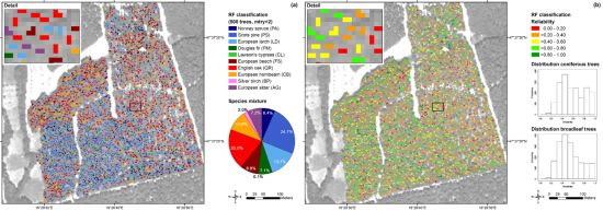
We classified the test area (Section 2.3) with the object-based RF approach (10 tree species, 8 bands). The classification results (majority votes) are shown in Figure 8(a). According to the forest stand map and our field observations, the test area is covered by a very heterogeneous mixed forest with equal proportions of coniferous and broadleaf tree species. The southwest is dominated by Scots pine and Norway spruce, and the eastern part is dominated by European beech. English oak, Silver birch, European alder, European hornbeam and European larch are also present serving as accompanying tree species. The classification results were plausible and corresponded quite well to this description. Likewise, the proportions of broadleaf and coniferous tree species were correctly determined.
The classification of Scots pine corresponded well to the observations in the field, whereas Norway spruce was underrepresented and European larch was overrepresented. According to the bootstrap results (Table 5), European larch showed one of the lowest classification accuracies due to confusion with Norway spruce and Scots pine. The tree crowns classified as Douglas fir were in fact Norway spruce. The Lawson’s cypress that was not present in the field, occurred only occasionally in the tree species map (<1%) showing that the classifier was mostly right regarding this tree species.
The classified crowns of European beech could be confirmed in the field to a very high degree. However, in total this tree species was underrepresented in the map. Furthermore, we observed that the proportion of English oak and European hornbeam in the map was higher than expected from the field observations. In some cases, this was due to confusion with European alder. The proportion of Silver birch corresponded well to our observations in the field.
For the reliability map presented in Figure 8(b) we computed the unambiguities and reliabilities according to Equations (2) and (3) using the classification results shown in Figure 8(a) and the user’s accuracies from Table 5. As shown in the histograms, the conifers were classified with a bit higher reliabilities (mean: 0.59) than the broadleaf trees (mean: 0.54). Among the conifers Scots pine was classified with the highest reliability (0.61) and European larch with the lowest (0.32). Among the broadleaf trees, European beech was classified with the highest reliability (0.58) and European hornbeam with the lowest (0.26). The tree species that were classified with a high reliability showed good agreement of the mapping results and the observations in the field.
4.7. Explanatory Power of the Spectral Bands
We examined the explanatory power of the 8 spectral bands in the classification of the 10 tree species using the following measures of variable importance: MDA, MDG, MDFC, and Wilks’ Lambda. For further interpretations, the measures of variable importance were evaluated in combination with the pairwise correlations shown in Table 2 and particularly under consideration of the 3 groups of bands identified on the basis of the correlation matrix. If a band is added to the set of variables that highly correlates with one of the bands that is already part of the variable set, only little additional information is provided by the new band, which may have an impact on the computed measures of variable importance.
Table 9 shows the explanatory power of the 8 bands according to the measures of variable importance derived from RF and LDA and the resulting band rankings.
The ranking according to MDG was similar to the ranking according to Wilks’ Lambda. Both measures ranked the bands Near Infrared 1, Near Infrared 2, Red Edge, and Green as the four most important variables. The ranking according to MDA and MDFC showed also some similarities. These two measures ranked the bands Green, Near Infrared 1, and Blue as the three most important variables. The bands Red and Near Infrared 2 were in the fourth position, respectively. As we can see from Table 9, one band per group was picked at a time. In this way, the band correlations were taken into account adding as much new spectral information as possible with each band.
We evaluated the measures of variable importance by simulating a feature selection procedure (Section 3.4). We compared the best classification result that could be achieved with 4 spectral bands (derived by trying out all 70 possible 4-band combinations) with the results achieved with the 4-band combinations proposed by MDA, MDG, MDFC, and Wilks’ Lambda (Table 10).
From the results presented in Table 10 we conclude that the feature selection according to MDA led to the best classification performance. Compared to the 4-band combination that gave the best classification result, the differences in overall accuracy were 1.5 percentage points with RF and 0.0 percentage points with LDA. The feature selection according to MDG and Wilks’ Lambda led to worse classification results. The poor classification performance of these 4-band combinations can be explained by the fact that in both cases 3 out of the 4 selected bands were highly correlated belonging to the same group (C) and that the spectral information represented by group A (Coastal, Blue) was missing. Wilks’ Lambda measures the explanatory power of the variables univariately. It does not consider the other variables in the feature set. Thus, if the feature set contains correlated variables, as it is the case in this study, Wilks’ Lambda is not suited for feature selection. Obviously, the same is valid for MDG, as it led to nearly the same band ranking. In contrast to Wilks’ Lambda, MDFC rates the variables multivariately (as it does MDA), but it led to a poorer classification performance than MDA (with a difference in overall accuracy of 3.9 percentage points with RF and 2.3 percentage points with LDA compared to the 4-band combination that gave the best classification result).
5. Discussion
5.1. Spectral Separability of Tree Species
The study shows that WorldView-2 satellite data are highly suitable to separate the investigated tree species. The distinction between coniferous and broadleaf tree species (RF, object-based, 10 tree species, 8 bands) was excellent (99% correct). The achieved user’s accuracies of the various tree species ranged between 57% and 92%, and the producer’s accuracies ranged between 33% and 94%. The lowest values were found for European hornbeam (CB) and European larch (LD). For these tree species it was difficult to find reliable reference samples, as they usually do not occur in pure stands in our study site. Therefore, some of the misclassifications maybe due to errors in the reference data set. Another possible reason for the observed misclassifications are spectral overlaps. The fact that some tree species reveal significantly lower accuracies, while other species show balanced classification results, are also found in other studies that considered a high number of tree species [12,60–64].
The classification of the test area showed some limitations. Concluding from our observations in the field, a great deal of the identified misclassifications could be explained by the very complex forest structure in the test area. Most stands were multi-storied and the tree crowns were small as the thinning was done only recently. Both characteristics lead to mixed pixels that may cause misclassifications.
In general, it was difficult to gather suitable data in the field for verification. Due to the described stand structure it was quite difficult to measure or estimate the tree species composition in the field in such a way that it was comparable with the one assessed from the image. The tree composition one can see and measure from the ground can vary significantly from the one seen from above. For this reason, we recommend visual (stereo) photo interpretation to obtain reliable quantitative data for verification rather than measurements in the field.
5.2. The Role of the 8 WorldView-2 Bands in Tree Species Classification
The 4 main tree species (Norway spruce (PA), Scots pine (PS), European beech (FS), and English oak (QR)) could be separated very accurately by using only the 4 standard bands (Blue, Green, Red, and Near infrared 1). Adding the 4 new bands (Coastal, Yellow, Red Edge, and Near infrared 2) to the set of explanatory variables had hardly any impact on the classification accuracy. This finding corresponds to the results of [10], where 4 bands and 8 bands performed almost equally in a two-class-problem using various classification algorithms (LDA, Quadratic Discriminant Analysis, Support Vector Machine and RF).
However, when we classified 10 tree species, the use of the 4 additional bands led to a significant improvement of classification accuracy. For example, in the object-based classification the Kappa value increased from 0.74 (4 bands) to 0.80 (8 bands). For two tree species (European larch (LD) and Douglas fir (PM)) the producer’s accuracies could be improved by more than 10 percentage points using all bands. Even stronger improvements could be achieved by [14]. They simulated WorldView-2 data from high spatial resolution hyperspectral data (High-fidelity Imaging Spectrometer, HiFIS) and reported an increase in Kappa from 0.55 to 0.71 (8 savanna tree species, maximum likelihood classification) by adding the 4 additional bands.
By including the 4 new bands in the set of explanatory variables, the number of variables used in the classification is doubled. From this, one may expect a stronger effect on classification accuracy than the one observed in our study. The small positive effect of the new bands can be explained by the pairwise band correlations. Each of the new bands correlated with one or more standard band(s) with a correlation coefficient higher than 0.85 (Coastal and Blue: 0.88, Yellow and Green: 0.90, Red Edge and Near Infrared 1: 0.95, Near Infrared 1 and Near Infrared 2: 0.98). Also the two new bands Red Edge and Near Infrared 2 showed a high correlation (0.95), whereas among the standard bands the correlations are low to moderate (0.02 to 0.77). Therefore adding the 4 new bands to the 4 standard bands introduced a lot of redundant information. One advantage of RF is that it can handle this collinearity [65].
An extensive analysis of the explanatory power of the bands revealed that in the classification with all 8 bands, the bands Green, Near Infrared 1, and Blue were most important. The bands Red (according to MDA) and Near Infrared 2 (according to MDFC) were in the fourth position. By checking all possible 4-band combinations, the combinations with the bands Coastal, Green, Red, and Near Infrared 1 (RF) and Blue, Green, Red, and Near Infrared 1 (LDA) yielded the best classification results. In all mentioned 4-band combinations at least 3 standard bands appear. From this we conclude that the new bands play only a minor part in tree species classification, but they are helpful especially when a larger number of tree species has to be separated or when the tree species show substantial spectral overlaps. The 4 measures of variable importance led to different 4-band combinations. With MDA, followed by MDFC, we could find the 4-band combinations that were closest to the optimal 4-band combination, whereas MDG and Wilks’ Lambda were not suitable for feature selection, as they score the bands without considering the information that the other variables in the feature set contribute. The superiority of MDA compared with MDG corresponds to the findings of [66,67]. They conclude that the MDA measure may be preferred, when within-predictor correlation exists.
5.3. Quality Checks
We introduced two new measures derived from the RF procedure for quality checking, the classification ambiguity and the classification reliability. Both indices were found very useful for interpreting the tree species map of the test site. The classification ambiguity permits to detect oddly behaving reference samples, i.e., outliers, very easily (validation phase). In the prediction phase it can be used in combination with the user’s accuracies to assess the classification reliability individually for each classified pixel or object. These measures are not restricted to tree species discrimination but can be helpful also for other problems such as land cover classification.
5.4. Non-Parametric versus Parametric Classification
The non-parametric RF classifier performed almost equally well as the established and widely used parametric LDA classifier. Comparing RF and LDA regarding their requirements on the data, we see the following advantages of RF for tree species classification: (1) In contrast to LDA, the non-parametric RF classifier does not make any assumptions about data distribution. Therefore it can handle also possibly occurring multi-modal data distributions. In our study the classes were mostly normally distributed leading to similar results with RF and LDA. However, this may not always be the case in image analysis. In tree species classification the robustness against non-normally distributed data sets can be helpful, for example, if only the most relevant tree species are mapped individually while pooling the secondary tree species in a single class. (2) RF is more flexible than LDA regarding class homogeneity. In contrast to LDA, RF does not require that the classes have a common covariance matrix, which often is not the case in tree species classification and hence limits the use of LDA and other parametric classifiers. (3) RF provides a reliable measure of variable importance, i.e., mean decrease in accuracy (MDA) that is very helpful for feature selection, as demonstrated in the paper. Altogether, RF offers a powerful alternative to traditional parametric methods.
5.5. Performance of the Pixel-Based and the Object-Based Approach
The object-based classification results outperformed the pixel-based results (10 tree species) in terms of overall accuracy by about 10 percentage points. These differences are notable especially considering that the results derived by the pixel-based approach might be positively biased due to spatial autocorrelation.
The advantage of classifying crown objects instead of individual pixels (both sunlit) corresponds to the findings in [5,10,38,39]. We assume that the average over a couple of pixels captures species-specific differences in crown structure and transmissivity very effectively and compensates for mixed pixels. The improvements achieved by object-based classification were higher for coniferous than for broadleaf trees (Figure 6(b)). This can be explained by differences in the crown form. Due to the conical shape of conifer crowns the sunlit regions are smaller and therefore more affected by mixed pixels compared to broadleaf trees with rather spherical crowns. Scots pine differs from other conifers showing an intermediate crown form. For this reason, the increase in accuracy observed for this tree species was least among the conifers.
As our tree crowns were usually covered only by a few 2 m pixels (multispectral), we could not take advantage of textural and/or n-dimensional co-variance information, as it is quite common in object-based classification. This approach proved already to be very efficient in physically-based retrievals of canopy LAI and other biophysical variables [68].
The performance of an object-based classification depends strongly on the quality of the segments. In this study, the crown delineation was done manually resulting in objects (i.e., tree crowns) that were ideally suited for classification. Reproducing this kind of delineation by using an automated segmentation algorithm is challenging but essential for an operational large-scale application of the method. The delineation of tree crowns can, for example, be done by auxiliary 3-D information [52,61,63,69–72], for example obtained from Canopy Height Models. Such datasets can either be derived from LiDAR data [52,61,69,71,73] or from the spectral images themselves [74] providing that they cover the area of interest stereoscopically. Other crown delineation approaches employ only spectral information and use different segmentation algorithms, such as (enhanced) watershed algorithms [75–77], multiresolution segmentation [11,63], or custom-built algorithms (e.g., [74,78–81]). A detailed overview of the different methods can be found for example in [82,83]. All studies use images with very high spatial resolution, preferably aerial photos. Therefore we expect that such approaches will also be suitable for WorldView-2 data that provide a panchromatic band with a pixel size of 0.5 m. The automatic tree crown delineation based on WorldView-2 data will be subject of further investigations.
Also for the pixel-based approach a procedure has to be established that automatically separates crown and non-crown pixels properly either during or previous to classification.
5.6. Comparison with Other Studies
The accuracies obtained in this study are in line with or higher than the accuracies reported in comparable studies. Table 11 presents an overview of studies on tree species classification in temperate and boreal forests carried out within the last 10 years using data from sensors with different spatial and spectral resolution. The applied classification algorithms range from parametric methods, such as logistic regression and the widely-used maximum likelihood classification, to nonparametric methods such as Support Vector Machines. The overall accuracies, reported in the listed studies, range between 45% and 96%. The highest values were generally achieved by analyzing only a small number of tree species and/or by using additional input data (e.g., LiDAR). In our study, the 4 main tree species Norway spruce, Scots pine, European beech and English oak were correctly classified with an overall accuracy of about 95%. This result is significantly better than the results reported in similar studies with 4 or 5 tree species. Also the classification of 10 tree species with an overall accuracy of 82% with RF and 84% with LDA respectively outperforms most of the other studies that included more than 5 tree species (Table 11).
We assume that the reasons for our relatively high classification accuracies were the spectral and spatial properties of the WorldView-2 sensor being very suitable for the task of tree species classification. Besides, the large sample size per class certainly had a positive impact on the classification results. Furthermore, we suppose that considering only the sunlit regions of the tree crowns in the classification process, as demonstrated also for other sensors [38,39,61,86], significantly contributed to high classification accuracies. In this way, the within-species spectral variability was not increased by varying illumination conditions within the tree crown. Finally, as we delineated the crowns manually, very accurate object boundaries were obtained. By this, the fusion of neighboring tree crowns in the reference polygons was avoided to a great extent resulting in almost unmixed reference samples.
6. Conclusion
The study focused on the suitability of single-date WorldView-2 data for tree species mapping at crown level in a mid-European forest test site located in Austria. For testing the sensor’s potential in forest mapping, a large number of individual tree crowns from 10 tree species were manually delineated. The retrieved spectral signatures were analyzed with the Random Forest (RF) classifier. For comparison the parametric Linear Discriminant Analysis (LDA) was also tested.
With an overall accuracy of 82% (RF, object-based, 10 tree species, 8 bands) we could demonstrate the high potential of WorldView-2 data for tree species mapping. The four new (additional) bands proved to be useful for classifying the full set of (10) tree species. However, the added-value of the new bands was species-dependent. Achieving improvements in user’s accuracy of 8 percentage points and higher, some tree species, such as Douglas fir and European larch, were much better separated with 8 bands, compared to the sole use of the 4 standard bands. For other tree species, such as Scots pine, European beech, Silver birch, and European alder, the improvements were only marginal (below 2 percentage points). As the 4 additional bands double the already very high (4-band) WorldView-2 data costs, users need to evaluate carefully, if the 4 new bands are beneficial in relation to the extra costs.
A few tree species showed significantly lower producer’s and user’s accuracies than the other species. For European hornbeam, for example, the user’s accuracy was only 57% (RF, object-based, 10 tree species, 8 bands), while for 8 of the 10 tree species it was 80% and higher. The relatively low accuracies were obtained despite the fact that the full spectral resolution of the WorldView-2 sensor was used and that the shadow effects were minimized by focusing only on the sunlit parts of the tree crowns. The observed spectral overlap is the result of the many structural and biochemical/biophysical variables determining the tree reflectance. This can yield similar spectral signatures with quite different combinations of structural and biochemical/biophysical properties. Perhaps, additional bands in the SWIR (reflectance spectra) or the TIR (emissivity spectra) would be needed for a better discrimination of these species. Hence, the WorldView-3 satellite, launching in 2014, with 8 new SWIR bands may improve the capabilities for tree species mapping. Alternatively, temporal and/or directional signatures could be analyzed in addition to the spectral data. Both additional dimensions are in principle obtainable from WorldView-2 data, but were not available for the present study.
RF and LDA can be considered representative and state-of-the-art classifiers for non-parametric and parametric algorithms. Both algorithms were similarly effective for the classification purpose. The main advantage of LDA is its straightforward interpretability. On the other hand, RF is probably more robust and theoretically more flexible regarding intra-class data distributions. In addition, the Mean Decrease in Accuracy (MDA) criterion, delivered as an output of RF, proved to be very efficient for feature selection. It performed slightly better than the corresponding metrics from LDA (Mean Discriminant Function Coefficient, MDFC) to identify the best 4-band combination out of all available 8 bands. The overall accuracy (RF, object-based, 10 tree species) that was achieved with the 4-band combination identified by MDA was only 1.5 percentage points lower than that achieved with the best 4-band combination. For this reason we recommend RF for similar studies and MDA for feature selection.
Our study clearly demonstrated the utility of deriving tree species related statistics reflecting the ambiguity of the class assignment. Benefits of such statistics were demonstrated for identifying possible misclassifications and outliers (e.g., erroneous and/or questionable references samples). Maps were produced indicating the unambiguity of the class assignment for each individual tree crown. Through field verification the usefulness of this quality measure was confirmed. Research in this direction should be continued.
Following a range of similar studies, our study focused on an object-based approach, where the pixel spectra within a delineated tree crown were averaged before analysis. For comparison, also pixel-based classification was tested and we could confirm the superiority of the object-based approach. We attribute the significant increase in overall accuracy of up to 10 percentage points (RF, 10 tree species, 8 bands) to the fact that the negative impact of mixed pixels was minimized by averaging the individual (pixel) signatures over the area covered by the sunlit tree crown. This interpretation is supported by the fact that the accuracy increase was most noticeable for conifers having relatively small sunlit regions per crown due to the conical shape of the crown. Small sunlit crown regions increase the risk of selecting mixed pixels affected by shadow effects. For similar studies, we therefore recommend object-based approaches.
As the WorldView-2 satellite was launched only in 2009, studies employing this new sensor for vegetation analysis are still rare. Only little information about the benefits and limitations of the 8 spectral bands are available. With this study we could contribute to fill this gap regarding tree species mapping. Our findings and conclusions refer to regions with forest conditions comparable with those in the presented study. Without additional studies, the results cannot be generalized. Further studies that cover different vegetation types within diverse bio-geographical settings are needed to confirm the potential of WorldView-2 data for tree species classification in other environments.
Supplementary
remotesensing-04-02661-s001.docxAcknowledgments
This study was partly funded by FFG (Austrian Research Promotion Agency). The authors would like to thank Umweltdata GmbH for providing the WorldView-2 image and the Esterházy forest enterprise for the forest management data. Special thanks also go to M. Mattiuzzi for his help with the software R. Finally, we acknowledge the helpful comments of four anonymous reviewers.
References
- Wulder, M.A.; Hall, R.J.; Coops, N.C.; Franklin, S.E. High spatial resolution remotely sensed data for ecosystem characterization. BioScience 2004, 54, 511–521. [Google Scholar]
- McDermid, G.J.; Hall, R.J.; Sanchez-Azofeifa, G.A.; Franklin, S.E.; Stenhouse, G.B.; Kobliuk, T.; LeDrew, E.F. Remote sensing and forest inventory for wildlife habitat assessment. For. Ecol. Manage 2009, 257, 2262–2269. [Google Scholar]
- Lindenmayer, D.B.; Margules, C.R.; Botkin, D.B. Indicators of biodiversity for ecologically sustainable forest management. Conserv. Biol 2000, 14, 941–950. [Google Scholar]
- Nagendra, H. Using remote sensing to assess biodiversity. Int. J. Remote Sens 2001, 22, 2377–2400. [Google Scholar]
- Clark, M.L.; Roberts, D.A.; Clark, D.B. Hyperspectral discrimination of tropical rain forest tree species at leaf to crown scales. Remote Sens. Environ 2005, 96, 375–398. [Google Scholar]
- Larsen, M. Single tree species classification with a hypothetical multi-spectral satellite. Remote Sens. Environ 2007, 110, 523–532. [Google Scholar]
- Warner, T.A.; Nellis, M.D.; Foody, G.M. Remote Sensing Scale and Data Selection Issues. In The SAGE Handbook of Remote Sensing; SAGE: Thousand Oaks, CA, USA, 2009; Volume 75, pp. 3–17. [Google Scholar]
- Koukal, T.; Atzberger, C. Potential of multi-angular data derived from a digital aerial frame camera for forest classification. IEEE J. Sel. Top. Appl 2012, 5, 30–43. [Google Scholar]
- DigitalGlobe, White Paper: The Benefits of the 8 Spectral Bands of WorldView-2; DigitalGlobe: Longmont, CO, USA, 2009.
- Chen, Q. Comparison of Worldview-2 and IKONOS-2 Imagery for Identifying Tree Species in the Habitat of an Endangered Bird Species in Hawaii; 8-Band Research Challenge; DigitalGlobe: Longmont, CO, USA, 2011. [Google Scholar]
- Sridharan, H. Multi-Level Comparison of WorldView-2 8-Band and AISA Hyperspectral Imageries for Urban Forest Classification; 8-Band Research Challenge; DigitalGlobe: Longmont, CO, USA, 2011. [Google Scholar]
- Omar, H. Commercial Timber Tree Species Identification Using Multispectral Worldview-2 Data; 8-Band Research Challenge; DigitalGlobe: Longmont, CO, USA, 2011. [Google Scholar]
- Latif, Z.A.; Zamri, I.; Omar, H. Determination of Tree Species Using Worldview-2 Data. Proceedings of IEEE 8th International Colloquium on Signal Processing and Its Applications (CSPA), Malacca, Malaysia, 23–25 March 2012; pp. 383–387.
- Cho, M.A.; Naidoo, L.; Mathieu, R.; Asner, G.P. Mapping Savanna Tree Species Using Carnegie Airborne Observatory Hyperspectral Data Resampled to WorldView-2 Multispectral Configuration. Proceedings of 34th International Symposium on Remote Sensing of Environment, Sydney, Australia, 10–15 April 2011.
- Duda, R.O.; Hart, P.E.; Stork, D.G. Pattern Classification, 2nd ed.; John Wiley & Sons: New York, NY, USA, 2000. [Google Scholar]
- Breiman, L. Random forests. Mach. Learn 2001, 45, 5–32. [Google Scholar]
- Hastie, T.; Tibshirani, R.; Friedman, J. The Elements of Statistical Learning: Data Mining, Inference, and Prediction, 2nd ed.; Springer: New York, NY, USA, 2009. [Google Scholar]
- Rodríguez-Galiano, V.F.; Ghimire, B.; Rogan, J.; Chica-Olmo, M.; Rigol-Sanchez, J.P. An assessment of the effectiveness of a random forest classifier for land-cover classification. ISPRS J. Photogramm 2012, 67, 93–104. [Google Scholar]
- Rodríguez-Galiano, V.F.; Abarca-Hernández, F.; Ghimire, B.; Chica-Olmo, M.; Atkinson, P.M.; Jeganathan, C. Incorporating spatial variability measures in land-cover classification using Random Forest. Procedia Envion. Sci 2011, 3, 44–49. [Google Scholar]
- Rodríguez-Galiano, V.F.; Chica-Olmo, M.; Abarca-Hernandez, F.; Atkinson, P.M.; Jeganathan, C. Random Forest classification of Mediterranean land cover using multi-seasonal imagery and multi-seasonal texture. Remote Sens. Environ 2012, 121, 93–107. [Google Scholar]
- Ghimire, B.; Rogan, J.; Miller, J. Contextual land-cover classification: Incorporating spatial dependence in land-cover classification models using Random Forests and the Getis statistic. Remote Sens. Lett 2010, 1, 45–54. [Google Scholar]
- Pal, M. Random forest classifier for remote sensing classification. Int. J. Remote Sens 2005, 26, 217–222. [Google Scholar]
- Miao, X.; Heaton, J.S.; Zheng, S.; Charlet, D.A.; Liu, H. Applying tree-based ensemble algorithms to the classification of ecological zones using multi-temporal multi-source remote-sensing data. Int. J. Remote Sens 2012, 33, 1823–1849. [Google Scholar]
- Clark, M.L.; Roberts, D.A. Species-level differences in hyperspectral metrics among tropical rainforest trees as determined by a tree-based classifier. Remote Sens 2012, 4, 1820–1855. [Google Scholar]
- Naidoo, L.; Cho, M.A.; Mathieu, R.; Asner, G. Classification of savanna tree species, in the Greater Kruger National Park region, by integrating hyperspectral and LiDAR data in a Random Forest data mining environment. ISPRS J. Photogramm. 2012, 69, 167–179. [Google Scholar]
- Lawrence, R.L.; Wood, S.D.; Sheley, R.L. Mapping invasive plants using hyperspectral imagery and Breiman Cutler classifications (randomForest). Remote Sens. Environ 2006, 100, 356–362. [Google Scholar]
- Dalponte, M.; Bruzzone, L.; Gianelle, D. Tree species classification in the Southern Alps based on the fusion of very high geometrical resolution multispectral/hyperspectral images and LiDAR data. Remote Sens. Environ 2012, 123, 258–270. [Google Scholar]
- Stumpf, A.; Kerle, N. Object-oriented mapping of landslides using Random Forests. Remote Sens. Environ 2011, 115, 2564–2577. [Google Scholar]
- Pierce, A.D.; Farris, C.A.; Taylor, A.H. Use of random forests for modeling and mapping forest canopy fuels for fire behavior analysis in Lassen Volcanic National Park, California, USA. For. Ecol. Manage 2012, 279, 77–89. [Google Scholar]
- Hudak, A.T.; Strand, E.K.; Vierling, L.A.; Byrne, J.C.; Eitel, J.U.H.; Martinuzzi, S.; Falkowski, M.J. Quantifying aboveground forest carbon pools and fluxes from repeat LiDAR surveys. Remote Sens. Environ 2012, 123, 25–40. [Google Scholar]
- Guo, L.; Chehata, N.; Mallet, C.; Boukir, S. Relevance of airborne lidar and multispectral image data for urban scene classification using Random Forests. ISPRS J. Photogramm 2011, 66, 56–66. [Google Scholar]
- Hughes, G. On the mean accuracy of statistical pattern recognizers. IEEE T. Inform. Theory 1968, 14, 55–63. [Google Scholar]
- Cortijo, F.J.; Perez De La Blanca, N. The performance of regularized discriminant analysis versus non-parametric classifiers applied to high-dimensional image classification. Int. J. Remote Sens 1999, 20, 3345–3365. [Google Scholar]
- Whiteside, T.G.; Boggs, G.S.; Maier, S.W. Comparing object-based and pixel-based classifications for mapping savannas. Int. J. Appl. Earth Obs. Geoinf 2011, 13, 884–893. [Google Scholar]
- Yan, G.; Mas, J.-F.; Maathuis, B.H.P.; Xiangmin, Z.; Van Dijk, P.M. Comparison of pixel-based and object-oriented image classification approaches—A case study in a coal fire area, Wuda, Inner Mongolia, China. Int. J. Remote Sens 2006, 27, 4039–4055. [Google Scholar]
- Weih, R.C., Jr.; Riggan, N.D., Jr. Object-Based Classification vs. Pixel-Based Classification: Comparitive Importance of Multi-Resolution Imagery. Proceedings of GEOBIA 2010: Geographic Object-Based Image Analysis, Ghent, Belgium, 29 June–2 July 2010; 38, Part 4/C7. p. 6.
- Kilian, W.; Müller, F.; Starlinger, F. Die Forstlichen Wuchsgebiete Österreichs: Eine Naturraumgliederung nach Waldökologischen; FBVA-Berichte; BFW: Vienna, Austria, 1994; p. 60. [Google Scholar]
- Leckie, D.G.; Tinis, S.; Nelson, T.; Burnett, C.; Gougeon, F.A.; Cloney, E.; Paradine, D. Issues in species classification of trees in old growth conifer stands. Can. J. Remote Sens 2005, 31, 175–190. [Google Scholar]
- Greenberg, J.A.; Dobrowski, S.Z.; Ramirez, C.M.; Tull, J.L.; Ustin, S.L. A bottom-up approach to vegetation mapping of the Lake Tahoe Basin using hyperspatial image analysis. Photogramm. Eng. Remote Sensing 2006, 72, 581–589. [Google Scholar]
- Updike, T.; Comp, C. Radiometric Use of WorldView-2 Imagery; DigitalGlobe: Longmont, CO, USA, 2010. [Google Scholar]
- Padwick, C.; Deskevich, M.; Pacifici, F.; Smallwood, S. WorldView-2 Pan-Sharpening. Proceedings of ASPRS 2010 Annual Conference, San Diego, CA, USA, 26–30 April 2010.
- Schlerf, M.; Atzberger, C. Vegetation structure retrieval in beech and spruce forests using spectrodirectional satellite data. IEEE J. Sel. Top. Appl 2012, 5, 8–17. [Google Scholar]
- Hosgood, B.; Jacquemoud, S.; Andreoli, G.; Verdebout, J.; Pedrini, G.; Schmuck, G. Leaf Optical Properties EXperiment 93 (LOPEX93); Report EUR 16095 EN; European Commission Joint Research Centre, Institute for Remote Sensing Applications: Ispra, Italy, 1994; p. 11. [Google Scholar]
- Kadro, A. Untersuchung der Spektralen Reflexionseigenschaften Verschiedener Vegetationsbestände, Ph.D. Dissertation, University Freiburg Freiburg im Breisgau, Germany. 1981.
- Breiman, L. Manual on Setting Up, Using, and Understanding Random Forests V3.1. 2002, p. 29. Available online: http://oz.berkeley.edu/users/breiman/Using_random_forests_V3.1.pdf (accessed on 5 May 2012).
- Liaw, A.; Wiener, M. Classification and regression by randomForest. R news 2002, 2, 18–22. [Google Scholar]
- Haara, A.; Haarala, M. Tree species classification using semi-automatic delineation of trees on aerial images. Scand. J. For. Res 2002, 17, 556–565. [Google Scholar]
- Feret, J.-B.; Asner, G.P.; Jacquemoud, S. Regularization of Discriminant Analysis for the Study of Biodiversity in Humid Tropical Forests. Proceedings of 2011 3rd Workshop on Hyperspectral Image and Signal Processing: Evolution in Remote Sensing (WHISPERS), Lisbon, Portugal, 6–9 June 2011; pp. 1–4.
- Brandtberg, T. Individual tree-based species classification in high spatial resolution aerial images of forests using fuzzy sets. Fuzzy Set. Syst 2002, 132, 371–387. [Google Scholar]
- Olofsson, K.; Wallerman, J.; Holmgren, J.; Olsson, H. Tree species discrimination using Z/I DMC imagery and template matching of single trees. Scand. J. For. Res 2006, 21, 106–110. [Google Scholar]
- Immitzer, M.; Atzberger, C.; Koukal, T. Eignung von WorldView-2 Satellitenbildern für die Baumartenklassifizierung unter besonderer Berücksichtigung der vier neuen Spektralkanäle. Photogramm. Fernerkun 2012, 2012, 573–588. [Google Scholar]
- Puttonen, E.; Litkey, P.; Hyyppä, J. Individual tree species classification by illuminated-shaded area separation. Remote Sens 2009, 2, 19–35. [Google Scholar]
- Efron, B. Estimating the error rate of a prediction rule: Improvement on cross-validation. J. Am. Stat. Assoc 1983, 78, 316–331. [Google Scholar]
- Cohen, J. A coefficient of agreement for nominal scales. Educ. Psychol. Meas 1960, 20, 37–46. [Google Scholar]
- Congalton, R.; Green, K. Assessing the Accuracy of Remotely Sensed Data Principles and Practices; Lewis: Boca Raton, FL, USA, 1999. [Google Scholar]
- Backhaus, K.; Erichson, B.; Plinke, W.; Weiber, R. Multivariate Analysemethoden: Eine anwendungsorientierte Einführung, 12th ed.; Springer: Berlin, Germany, 2008. [Google Scholar]
- R Development Core Team, R: A Language and Environment for Statistical Computing; R Foundation for Statistical Computing: Vienna, Austria, 2012.
- Nakazawa, M. fmsb: Functions for Medical Statistics Book with Some Demographic Data, R Package Version 0.3.4; 2012. Available online: http://CRAN.R-project.org/package=fmsb (accessed on 9 August 2012).
- Venables, W.N.; Ripley, B.D. Modern Applied Statistics with S, 4th ed; Springer: New York, NY, USA, 2002. [Google Scholar]
- Carleer, A.; Wolff, E. Exploitation of very high resolution satellite data for tree species identification. Photogramm. Eng. Remote Sensing 2004, 70, 135–140. [Google Scholar]
- Waser, L.T.; Ginzler, C.; Kuechler, M.; Baltsavias, E.; Hurni, L. Semi-automatic classification of tree species in different forest ecosystems by spectral and geometric variables derived from Airborne Digital Sensor (ADS40) and RC30 data. Remote Sens. Environ 2011, 115, 76–85. [Google Scholar]
- Waser, L.T.; Klonus, S.; Ehlers, M.; Küchler, M.; Jung, A. Potential of digital sensors for land cover and tree species classifications—A case study in the framework of the DGPF-project. Photogramm. Fernerkun 2010, 2010, 141–156. [Google Scholar]
- Voss, M.; Sugumaran, R. Seasonal effect on tree species classification in an urban environment using hyperspectral data, LiDAR, and an object-oriented approach. Sensors 2008, 8, 3020–3036. [Google Scholar]
- Jones, T.G.; Coops, N.C.; Sharma, T. Assessing the utility of airborne hyperspectral and LiDAR data for species distribution mapping in the coastal Pacific Northwest, Canada. Remote Sens. Environ 2010, 114, 2841–2852. [Google Scholar]
- Mendez, G.; Buskirk, T.D.; Lohr, S.; Haag, S. Factors associated with persistence in science and engineering majors: An exploratory study using classification trees and random forests. J. Eng. Educ 2008, 97, 57–69. [Google Scholar]
- Nicodemus, K.K.; Malley, J.D. Predictor correlation impacts machine learning algorithms: Implications for genomic studies. Bioinformatics 2009, 25, 1884–1890. [Google Scholar]
- Nicodemus, K.K. Letter to the editor: on the stability and ranking of predictors from random forest variable importance measures. Brief Bioinform 2011, 12, 369–373. [Google Scholar]
- Atzberger, C.; Richter, K. Spatially constrained inversion of radiative transfer models for improved LAI mapping from future Sentinel-2 imagery. Remote Sens. Environ 2012, 120, 208–218. [Google Scholar]
- Holmgren, J.; Persson, Å.; Söderman, U. Species identification of individual trees by combining high resolution LiDAR data with multi-spectral images. Int. J. Remote Sens 2008, 29, 1537–1552. [Google Scholar]
- Dalponte, M.; Bruzzone, L.; Gianelle, D. Fusion of hyperspectral and LIDAR remote sensing data for classification of complex forest areas. IEEE Trans Geosci. Remote Sens 2008, 46, 1416–1427. [Google Scholar]
- Straub, C.; Weinacker, H.; Koch, B. A comparison of different methods for forest resource estimation using information from airborne laser scanning and CIR orthophotos. Eur. J. For. Res 2010, 129, 1069–1080. [Google Scholar]
- Erins, G.; Lorencs, A.; Mednieks, I.; Sinica-Sinavskis, J. Tree Species Classification in Mixed Baltic Forest. Proceedings of 2011 3rd Workshop on Hyperspectral Image and Signal Processing: Evolution in Remote Sensing (WHISPERS), Lisbon, Portugal, 6–9 June 2011; pp. 1–4.
- Heinzel, J.N.; Weinacker, H.; Koch, B. Full Automatic Detection of Tree Species Based on Delineated Single Tree Crowns—A Data Fusion Approach for Airborne Laser Scanning Data and Aerial Photographs. Proceedings of SilviLaser 8th International Conference on LiDAR Applications in Forest Assessment and Inventory, Edinburgh, UK, 17–19 September 2008; pp. 76–85.
- Brandtberg, T. Automatic individual tree based analysis of high spatial resolution aerial images on naturally regenerated boreal forests. Can. J. For. Res 1999, 29, 1464–1478. [Google Scholar]
- Kanda, F.; Kubo, M.; Muramoto, K. Watershed Segmentation and Classification of Tree Species Using High Resolution Forest Imagery. Proceedings of 2004 IEEE International Geoscience and Remote Sensing Symposium, Anchorage, AK, USA, 20–24 September 2004; Volume 6. pp. 3822–3825.
- Wang, L.; Gong, P.; Biging, G.S. Individual tree-crown delineation and treetop detection in high-spatial-resolution aerial imagery. Photogramm. Eng. Remote Sensing 2004, 70, 351–357. [Google Scholar]
- Niccolai, A.; Hohl, A.; Niccolai, M.; Oliver, C.D. Integration of varying spatial, spectral and temporal high-resolution optical images for individual tree crown isolation. Int. J. Remote Sens 2010, 31, 5061–5088. [Google Scholar]
- Culvenor, D.S. TIDA: An algorithm for the delineation of tree crowns in high spatial resolution remotely sensed imagery. Comput. Geosci 2002, 28, 33–44. [Google Scholar]
- Erikson, M. Segmentation of individual tree crowns in colour aerial photographs using region growing supported by fuzzy rules. Can. J. For. Res 2003, 33, 1557–1563. [Google Scholar]
- Leckie, D.G.; Gougeon, F.A.; Tinis, S.; Nelson, T.; Burnett, C.N.; Paradine, D. Automated tree recognition in old growth conifer stands with high resolution digital imagery. Remote Sens. Environ 2005, 94, 311–326. [Google Scholar]
- Katoh, M.; Gougeon, F.A. Improving the precision of tree counting by combining tree detection with crown delineation and classification on homogeneity guided smoothed high resolution (50 cm) multispectral airborne digital data. Remote Sens 2012, 4, 1411–1424. [Google Scholar]
- Culvenor, D.S. Extracting Individual Tree Information: A Survey of Techniques for High Spatial Resolution Imagery. In Remote Sensing of Forest Environments: Concepts and Case Studies; Wulder, M.A., Franklin, S.E., Eds.; Kluwer Academic Publishers: Norwell, MA, USA, 2003; pp. 255–277. [Google Scholar]
- Wolf, B.-M.; Heipke, C. Automatic extraction and delineation of single trees from remote sensing data. Mach. Vision Appl 2007, 18, 317–330. [Google Scholar]
- Korpela, I. Individual Tree Measurements by Means of Digital Aerial Photogrammetry; Silva Fennica Monographs 3; Finnish Society of Forest Science: Helsinki, Finland, 2004. [Google Scholar]
- Heikkinen, V.; Korpela, I.; Tokola, T.; Honkavaara, E.; Parkkinen, J. An SVM classification of tree species radiometric signatures based on the Leica ADS40 sensor. IEEE Trans. Geosci. Remote Sens 2011, 49, 4539–4551. [Google Scholar]
- Erikson, M. Species classification of individually segmented tree crowns in high-resolution aerial images using radiometric and morphologic image measures. Remote Sens. Environ 2004, 91, 469–477. [Google Scholar]
- Stoffels, J.; Mader, S.; Hill, J.; Werner, W.; Ontrup, G. Satellite-based stand-wise forest cover type mapping using a spatially adaptive classification approach. Eur. J. For. Res 2012, 4, 1071–1089. [Google Scholar]
- Leckie, D.G.; Gougeon, F.A.; Walsworth, N.; Paradine, D. Stand delineation and composition estimation using semi-automated individual tree crown analysis. Remote Sens. Environ 2003, 85, 355–369. [Google Scholar]
- Hill, R.A.; Wilson, A.K.; George, M.; Hinsley, S.A. Mapping tree species in temperate deciduous woodland using time-series multi-spectral data. Appl. Veg. Sci 2010, 13, 86–99. [Google Scholar]
- Kim, S.-R.; Lee, W.-K.; Kwak, D.-A.; Biging, G.S.; Gong, P.; Lee, J.-H.; Cho, H.-K. Forest cover classification by optimal segmentation of high resolution satellite imagery. Sensors 2011, 11, 1943–1958. [Google Scholar]
- Boschetti, M.; Boschetti, L.; Oliveri, S.; Casati, L.; Canova, I. Tree species mapping with airborne hyper-spectral MIVIS data: The Ticino Park study case. Int. J. Remote Sens 2007, 28, 1251–1261. [Google Scholar]
- Dalponte, M.; Bruzzone, L.; Gianelle, D. Tree Species Classification in the Southern Alps with Very High Geometrical Resolution Multispectral and Hyperspectral Data. Proceedings of 2011 3rd Workshop on Hyperspectral Image and Signal Processing: Evolution in Remote Sensing (WHISPERS), Lisbon, Portugal, 6–9 June 2011; pp. 1–4.
Figure 1.
Study site, test area and location of reference samples (homogeneous stands).
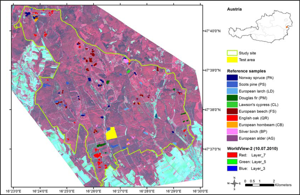
Figure 2.
Manual delineation of sunlit tree crowns exemplified for the test area: (a) selected tree crowns in the image with 0.5 m pixel size, and (b) derived tree crown polygons in the image with 2 m pixel size.
Figure 2.
Manual delineation of sunlit tree crowns exemplified for the test area: (a) selected tree crowns in the image with 0.5 m pixel size, and (b) derived tree crown polygons in the image with 2 m pixel size.
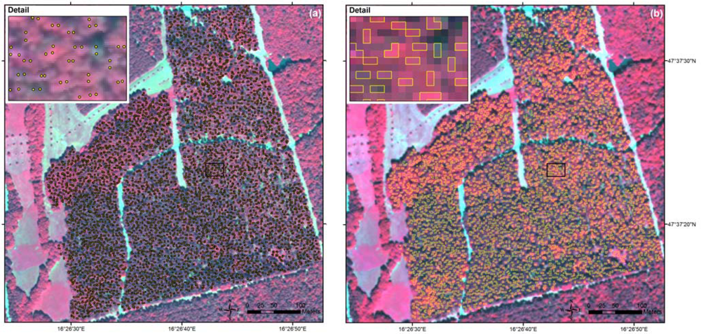
Figure 3.
Mean spectral signatures of the 10 tree species derived from the 8 WorldView-2 bands using the reference polygons (for sample size see Table 1): (a) full spectrum, and (b) wavelength range of visible light (detail of the full spectrum).
Figure 3.
Mean spectral signatures of the 10 tree species derived from the 8 WorldView-2 bands using the reference polygons (for sample size see Table 1): (a) full spectrum, and (b) wavelength range of visible light (detail of the full spectrum).

Figure 4.
Box-whisker-plots of median reflectance values of the 8 WorldView-2 bands for the 10 tree species derived from the reference polygons.
Figure 4.
Box-whisker-plots of median reflectance values of the 8 WorldView-2 bands for the 10 tree species derived from the reference polygons.

Figure 5.
Effect of the number of trees and the number of random split variables at each node (mtry) on the overall accuracy for the object-based RF classification of 10 tree species using the 8 bands of WorldView-2 (mean overall accuracy from 20 repetitions).
Figure 5.
Effect of the number of trees and the number of random split variables at each node (mtry) on the overall accuracy for the object-based RF classification of 10 tree species using the 8 bands of WorldView-2 (mean overall accuracy from 20 repetitions).

Figure 6.
Spider charts representing the user’s accuracies for the following classification approaches (RF, 10 tree species): (a) 8 versus 4 bands (object-based), (b) object-based versus pixel-based (8 bands).
Figure 6.
Spider charts representing the user’s accuracies for the following classification approaches (RF, 10 tree species): (a) 8 versus 4 bands (object-based), (b) object-based versus pixel-based (8 bands).
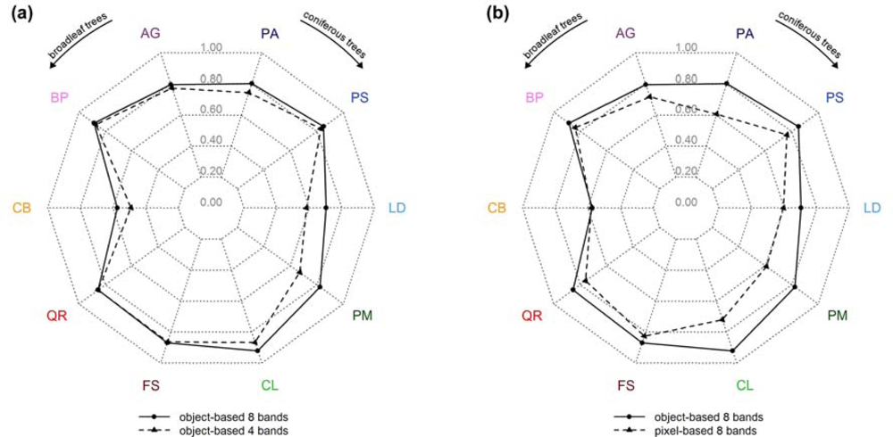
Figure 7.
Histograms based on the classification unambiguity for (a) coniferous and (b) broadleaf trees ranging from 0 to 1 with an interval of 0.1 for the three cases (case a: correctly classified samples of the specified tree species, case b: samples of the specified tree species classified as another tree species, and case c: samples of other tree species classified as the specified tree species).
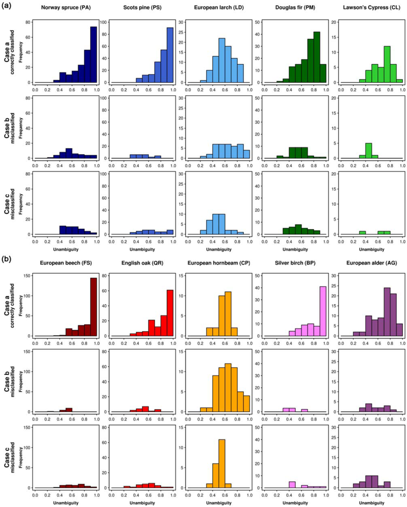
Figure 8.
Classification of the test area (RF, 10 tree species, 8 bands): (a) tree species map, (b) reliability map derived from the species-specific user’s accuracies and the individual unambiguities.
Figure 8.
Classification of the test area (RF, 10 tree species, 8 bands): (a) tree species map, (b) reliability map derived from the species-specific user’s accuracies and the individual unambiguities.


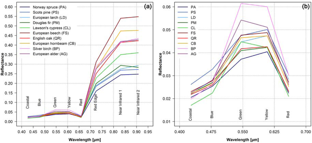
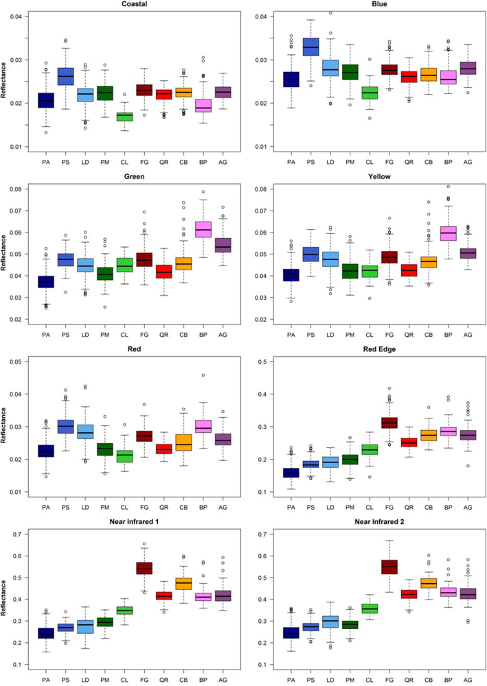
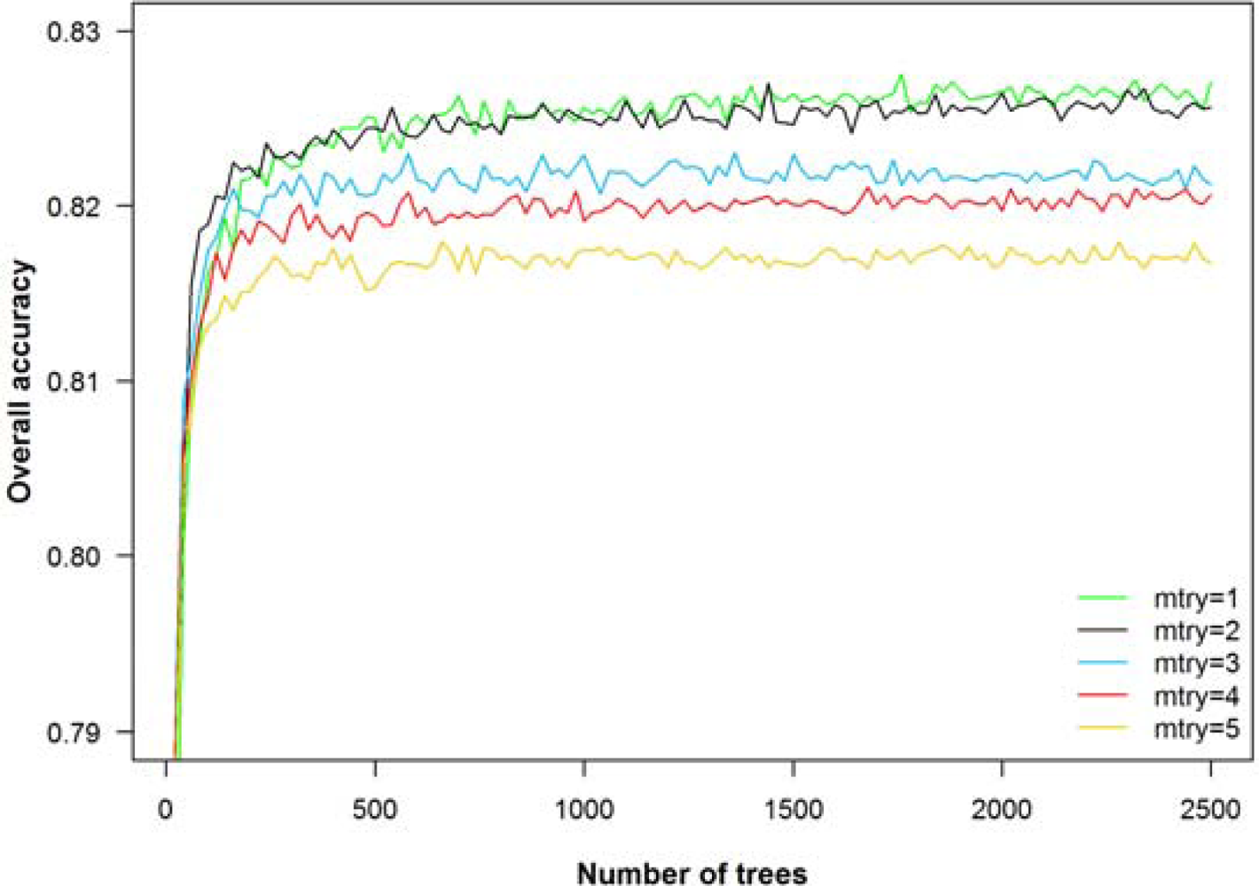
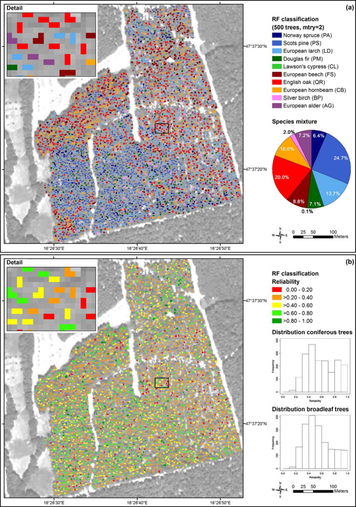
Table 1.
Common and scientific names, acronyms, and number of pixels and objects of the 10 analyzed tree species.
| Common Name | Scientific Name | Acronym | Type | Leaf Phenology | No. of Pixels | No. of Objects | Proportion1 [%] |
|---|---|---|---|---|---|---|---|
| Norway spruce | Picea abies | PA | Conifer | Evergreen | 1,084 | 226 | 15.4 |
| Scots pine | Pinus sylvestris | PS | Conifer | Evergreen | 807 | 235 | 16.0 |
| European larch | Larix decidua | LD | Conifer | Deciduous | 472 | 122 | 8.3 |
| Douglas fir | Pseudotsuga menziesii | PM | Conifer | Evergreen | 677 | 178 | 12.1 |
| Lawson’s cypress | Chamaecyparis lawsoniana | CL | Conifer | Evergreen | 166 | 42 | 2.9 |
| European beech | Fagus sylvatica | FS | Broadleaf | Deciduous | 1,519 | 247 | 16.9 |
| English oak | Quercus robur | QR | Broadleaf | Deciduous | 1,770 | 152 | 10.4 |
| European hornbeam | Carpinus betulus | CB | Broadleaf | Deciduous | 445 | 81 | 5.5 |
| Silver birch | Betula pendula | BP | Broadleaf | Deciduous | 397 | 86 | 5.9 |
| European alder | Alnus glutinosa | AG | Broadleaf | Deciduous | 387 | 96 | 6.6 |
| 7,724 | 1,465 | 100.0 | |||||
1based on objects.
Table 2.
Pairwise correlations between the 8 bands computed from the reference samples (the names of the new bands are printed in cursive letters, correlations >0.70 in bold letters).
| Group | Band | Coastal | Blue | Green | Yellow | Red | Red Edge | Near Infrared 1 | Near Infrared 2 |
|---|---|---|---|---|---|---|---|---|---|
| A | Coastal | - | 0.88 | 0.36 | 0.48 | 0.64 | 0.11 | 0.08 | 0.06 |
| Blue | 0.88 | - | 0.48 | 0.57 | 0.77 | 0.05 | −0.02 | −0.04 | |
| B | Green | 0.36 | 0.48 | - | 0.90 | 0.72 | 0.61 | 0.44 | 0.45 |
| Yellow | 0.48 | 0.57 | 0.90 | - | 0.82 | 0.51 | 0.33 | 0.35 | |
| Red | 0.64 | 0.77 | 0.72 | 0.82 | - | 0.26 | 0.14 | 0.16 | |
| C | Red Edge | 0.11 | 0.05 | 0.61 | 0.51 | 0.26 | - | 0.95 | 0.95 |
| Near Infrared 1 | 0.08 | −0.02 | 0.44 | 0.33 | 0.14 | 0.95 | - | 0.98 | |
| Near Infrared 2 | 0.06 | −0.04 | 0.45 | 0.35 | 0.16 | 0.95 | 0.98 | - | |
| Case | Majority vote | Reference | Classified as |
|---|---|---|---|
| a | correct | tree species i | tree species i |
| b | wrong | tree species i | not tree species i |
| c | wrong | not tree species i | tree species i |
Table 4.
Confusion matrix for the 4 main tree species using the 8 bands of WorldView-2 and object-based RF classification (horizontal line separates coniferous and broadleaf trees).
| Reference Data | ||||||
|---|---|---|---|---|---|---|
| Classified as | PA | PS | FS | QR | Σ | User’s acc. |
| PA | 211 | 12 | 0 | 0 | 223 | 0.946 |
| PS | 15 | 223 | 0 | 0 | 238 | 0.937 |
| FS | 0 | 0 | 243 | 4 | 247 | 0.980 |
| QR | 0 | 0 | 4 | 148 | 152 | 0.974 |
| Σ | 226 | 235 | 247 | 152 | 860 | |
| Prod. acc. | 0.934 | 0.949 | 0.984 | 0.974 | 0.959 | |
Table 5.
Confusion matrix for the 10 tree species using the 8 bands of WorldView-2 and object-based RF classification (horizontal line separates coniferous and broadleaf trees).
| Reference Data | ||||||||||||
|---|---|---|---|---|---|---|---|---|---|---|---|---|
| Classified as | PA | PS | LD | PM | CL | FS | QR | CB | BP | AG | Σ | User’s acc. |
| PA | 181 | 8 | 18 | 17 | 1 | 0 | 0 | 0 | 0 | 0 | 225 | 0.804 |
| PS | 11 | 211 | 18 | 8 | 0 | 0 | 0 | 0 | 0 | 0 | 248 | 0.851 |
| LD | 10 | 14 | 81 | 8 | 1 | 0 | 0 | 0 | 0 | 1 | 115 | 0.704 |
| PM | 24 | 2 | 4 | 144 | 0 | 0 | 0 | 0 | 0 | 1 | 175 | 0.823 |
| CL | 0 | 0 | 0 | 0 | 35 | 0 | 0 | 0 | 1 | 2 | 38 | 0.921 |
| FS | 0 | 0 | 0 | 0 | 0 | 233 | 1 | 28 | 3 | 3 | 268 | 0.869 |
| QR | 0 | 0 | 1 | 0 | 0 | 2 | 135 | 15 | 0 | 5 | 158 | 0.854 |
| CB | 0 | 0 | 0 | 0 | 0 | 11 | 9 | 27 | 0 | 0 | 47 | 0.574 |
| BP | 0 | 0 | 0 | 0 | 1 | 1 | 0 | 6 | 78 | 2 | 88 | 0.886 |
| AG | 0 | 0 | 0 | 1 | 4 | 0 | 7 | 5 | 4 | 82 | 103 | 0.796 |
| Σ | 226 | 235 | 122 | 178 | 42 | 247 | 152 | 81 | 86 | 96 | 1465 | |
| Prod. acc. | 0.801 | 0.898 | 0.664 | 0.809 | 0.833 | 0.943 | 0.888 | 0.333 | 0.907 | 0.854 | 0.824 | |
Table 6.
Confusion matrix for the 10 tree species using the 4 standard bands of WorldView-2 and object-based RF classification (horizontal line separates coniferous and broadleaf trees).
| Reference Data | ||||||||||||
|---|---|---|---|---|---|---|---|---|---|---|---|---|
| Classified as | PA | PS | LD | PM | CL | FS | QR | CB | BP | AG | Σ | User’s acc. |
| PA | 167 | 7 | 20 | 29 | 1 | 0 | 0 | 0 | 0 | 0 | 224 | 0.746 |
| PS | 10 | 204 | 24 | 8 | 0 | 0 | 0 | 0 | 0 | 0 | 246 | 0.829 |
| LD | 11 | 17 | 63 | 14 | 1 | 0 | 0 | 1 | 0 | 1 | 108 | 0.583 |
| PM | 38 | 7 | 12 | 124 | 3 | 0 | 1 | 0 | 0 | 0 | 185 | 0.670 |
| CL | 0 | 0 | 0 | 2 | 33 | 0 | 0 | 0 | 0 | 3 | 38 | 0.868 |
| FS | 0 | 0 | 0 | 0 | 0 | 227 | 1 | 31 | 1 | 3 | 263 | 0.863 |
| QR | 0 | 0 | 1 | 1 | 0 | 2 | 140 | 15 | 0 | 5 | 164 | 0.854 |
| CB | 0 | 0 | 1 | 0 | 0 | 17 | 6 | 24 | 1 | 0 | 49 | 0.490 |
| BP | 0 | 0 | 0 | 0 | 0 | 1 | 0 | 5 | 75 | 5 | 86 | 0.872 |
| AG | 0 | 0 | 1 | 0 | 4 | 0 | 4 | 5 | 9 | 79 | 102 | 0.775 |
| Σ | 226 | 235 | 122 | 178 | 42 | 247 | 152 | 81 | 86 | 96 | 1465 | |
| Prod. acc. | 0.739 | 0.868 | 0.516 | 0.697 | 0.786 | 0.919 | 0.921 | 0.296 | 0.872 | 0.823 | 0.775 | |
Table 7.
Confusion matrix for the 10 tree species using the 8 bands of WorldView-2 and pixel-based RF classification (horizontal line separates coniferous and broadleaf trees).
| Reference Data | ||||||||||||
|---|---|---|---|---|---|---|---|---|---|---|---|---|
| Classified as | PA | PS | LD | PM | CL | FS | QR | CB | BP | AG | Σ | User’s acc. |
| PA | 755 | 125 | 143 | 186 | 4 | 3 | 12 | 1 | 6 | 9 | 1244 | 0.607 |
| PS | 109 | 629 | 51 | 30 | 0 | 0 | 4 | 1 | 0 | 0 | 824 | 0.763 |
| LD | 41 | 28 | 202 | 35 | 5 | 1 | 11 | 5 | 9 | 2 | 339 | 0.596 |
| PM | 141 | 21 | 48 | 393 | 12 | 0 | 21 | 0 | 5 | 5 | 646 | 0.608 |
| CL | 4 | 0 | 1 | 6 | 103 | 1 | 2 | 1 | 17 | 8 | 143 | 0.720 |
| FS | 0 | 0 | 1 | 0 | 0 | 1330 | 89 | 165 | 6 | 19 | 1610 | 0.826 |
| QR | 27 | 3 | 15 | 22 | 15 | 154 | 1589 | 167 | 16 | 86 | 2094 | 0.759 |
| CB | 0 | 0 | 0 | 0 | 0 | 26 | 15 | 70 | 6 | 4 | 121 | 0.579 |
| BP | 0 | 1 | 3 | 2 | 15 | 0 | 1 | 23 | 310 | 15 | 370 | 0.838 |
| AG | 7 | 0 | 8 | 3 | 12 | 4 | 26 | 12 | 22 | 239 | 333 | 0.718 |
| Σ | 1084 | 807 | 472 | 677 | 166 | 1519 | 1770 | 445 | 397 | 387 | 7724 | |
| Prod. acc. | 0.696 | 0.779 | 0.428 | 0.581 | 0.620 | 0.876 | 0.898 | 0.157 | 0.781 | 0.618 | 0.728 | |
Table 8.
Classification results with 4 and 8 bands for the 4 main tree species (PA, PS, FS, QR) and all 10 tree species (PA, PS, LD, PM, CL, FS, QR, CB, BP, AG), for the pixel-based and the object-based approach and for the two classification algorithms (RF and LDA).
| Tree Species | Approach | WorldView-2 Bands1 | RF | LDA | ||
|---|---|---|---|---|---|---|
| Overall acc. | Kappa | Overall acc. | Kappa | |||
| 4 | pixel-based | 4 (B,G,R,NIR1) | 0.868 | 0.819 | 0.849 | 0.793 |
| 8 (C,B,G,Y,R,RE,NIR1,NIR2) | 0.881 | 0.837 | 0.862 | 0.810 | ||
| object-based | 4 (B,G,R,NIR1) | 0.955 | 0.939 | 0.949 | 0.931 | |
| 8 (C,B,G,Y,R,RE,NIR1,NIR2) | 0.959 | 0.945 | 0.944 | 0.925 | ||
| 10 | pixel-based | 4 (B,G,R,NIR1) | 0.690 | 0.634 | 0.657 | 0.593 |
| 8 (C,B,G,Y,R,RE,NIR1,NIR2) | 0.728 | 0.678 | 0.700 | 0.645 | ||
| object-based | 4 (B,G,R,NIR1) | 0.775 | 0.743 | 0.786 | 0.756 | |
| 8 (C,B,G,Y,R,RE,NIR1,NIR2) | 0.824 | 0.799 | 0.835 | 0.811 | ||
1C: Coastal, B: Blue, G: Green, Y: Yellow, R: Red, RE: Red Edge, NIR1: Near Infrared 1, NIR2: Near Infrared 2.
Table 9.
Explanatory power of the 8 bands in the classification of the 10 tree species from different statistical analysis (MDA & MDG: RF, MDFC: LDA, Wilks’ Lambda: ANOVA) with the corresponding ranks in parentheses. The horizontal lines separate the 3 groups identified on the basis of the correlation matrix (new bands are printed in cursive letters).
| Band | Group | MDA | MDG | MDFC | Wilks’ Lambda |
|---|---|---|---|---|---|
| Coastal | A | 0.896 (5) | 117.8 (8) | 0.295 (5) | 0.580 (8) |
| Blue | 0.899 (3) | 130.9 (6) | 0.407 (3) | 0.507 (7) | |
| Green | B | 0.909 (1) | 145.2 (4) | 0.470 (2) | 0.392 (4) |
| Yellow | 0.876 (7) | 118.0 (7) | 0.257 (6) | 0.471 (5) | |
| Red | 0.898 (4) | 132.0 (5) | 0.256 (7) | 0.495 (6) | |
| Red Edge | C | 0.858 (8) | 184.0 (3) | 0.183 (8) | 0.154 (3) |
| Near Infrared 1 | 0.903 (2) | 238.3 (1) | 0.650 (1) | 0.096 (1) | |
| Near Infrared 2 | 0.887 (6) | 219.1 (2) | 0.361 (4) | 0.099 (2) | |
Table 10.
Overall accuracies for RF (mean overall accuracy from 20 repetitions) and LDA (with all samples) derived by different 4-band combinations (new bands are printed in cursive letters) based on MDA, MDG, MDFC, and Wilks’ Lambda (10 tree species, object-based).
| Basis of the 4-Band Combination | 4-Band Combination1 | Overall acc. RF | Overall acc. LDA |
|---|---|---|---|
| best classification result RF | C, G, R, NIR1 | 0.792 | 0.782 |
| best classification result LDA | B, G, R, NIR1 | 0.777 | 0.790 |
| MDA | B, G, R, NIR1 | 0.777 | 0.790 |
| MDG | G, RE, NIR1, NIR2 | 0.726 | 0.746 |
| MDFC | B, G, NIR1, NIR2 | 0.753 | 0.767 |
| Wilks’ Lambda | G, RE, NIR1, NIR2 | 0.726 | 0.746 |
1C: Coastal, B: Blue, G: Green, Y: Yellow, R: Red, RE: Red Edge, NIR1: Near Infrared 1, NIR2: Near Infrared 2
Table 11.
Results from tree species classifications in temperate and boreal forests with spectral remote sensing data using different sensors and classification methods from the last 10 years (ordered by the number of tree species and overall accuracy).
| Platform1 | Datatyp2 | Sensor | Acquisition date | LiDAR3 | Classification algorithm4 | Approach5 | Species no. | Overall acc. [%]6 | Kappa6 | Tree species | Reference |
|---|---|---|---|---|---|---|---|---|---|---|---|
| A | M | DMC | Jun | x | ML | OI | 3 | 96 | 0.93 | Picea abies, Pinus sylvestris & broadleaf trees | [69] |
| A | M | DMC | Oct | ML | OI | 3 | 91 | 0.87 | Picea abies, Pinus sylvestris & broadleaf trees | [69] | |
| A | M | Wild RC 20 | May & Jul | MD | OI | 3 | 91 | 0.86 | Picea abies, Pinus sylvestris & Betula pendula | [84] | |
| A | M | DMC | Oct | LDA | OI | 3 | 89 | 0.82 | Picea abies, Pinus sylvestris & broadleaf trees | [50] | |
| A | M | ADS40-SH52 | Aug | SVM | OI | 3 | 88 | n.s. | Pinus sylvestris, Picea abies & Betula sp. | [85] | |
| H | M | DCRTRV20 | Oct | ML | OS | 3 | 87 | n.s. | Larix sp., Cryptomeria japonica, Fagus sp. | [75] | |
| A | M | DMC | Jun | ML | OI | 3 | 84 | 0.76 | Picea abies, Pinus sylvestris & broadleaf trees | [69] | |
| A | M | n.s. | n.s. | x | DT | OI | 3 | 84 | n.s. | Fagus sylvatica, Quercus sp. / Carpinus betulus & conifers | [73] |
| A | M | Wild RC 20 | Jun | LDA | OI | 3 | 78 | n.s. | Picea abies, Pinus sylvestris & broadleaf trees | [47] | |
| A | M | DMC | Sep | LDA | OI | 3 | 68 | n.s. | Picea abies, Pinus sylvestris & Betula sp. | [52] | |
| A | M | ADS40-SH52 | Sep | ANN | OI | 4 | 84 | 0.73 | Picea abies, Pinus sylvestris, Larix decidua & Betula sp. | [61] | |
| A | M | Wild RC30/4 | Aug | DT | OI | 4 | 77 | n.s. | Picea abies, Pinus sylvestris, Betula pubescens & Populus tremula | [86] | |
| A | M | n.s. | Aug | LDA | OI | 4 | 67 | n.s. | Picea abies, Pinus sylvestris, Betula pubescens & Populus tremula | [49] | |
| S | M | ASTER | Apr & Jun | ACA | OS | 5 | 87 | 0.83 | Picea abies, Pinus sylvestris, Pseudotsuga menziesii, Fagus sylvatica, & Quercus sp. | [87] | |
| S | M | ASTER | Apr & Jun | ML | OS | 5 | 82 | 0.77 | Picea abies, Pinus sylvestris, Pseudotsuga menziesii, Fagus sylvatica, & Quercus sp. | [87] | |
| A | M | CASI | Sep | ML | OI | 6 | 93 | n.s. | Pseudotsuga menziesii, Abies grandis, Abies amabilis, Thuja plicata, Tsuga heterophylla & hardwood | [88] | |
| A | M | ATM | Oct | ML | OI | 6 | 84 | 0.79 | Fraxinus excelsior, Quercus robur, Acer campestre, Betula pendula, Populus tremula & Ulmus minor | [89] | |
| A | M | ATM | Mar, Jul & Oct | ML | OI | 6 | 71 | 0.63 | Fraxinus excelsior, Quercus robur, Acer campestre, Betula pendula, Populus tremula & Ulmus minor | [89] | |
| A | H | AISA | Jul | x | NN | OI | 6 | 57 | n.s. | Pinus strobus, Picea glauca, Gleditsia triacanthos, Acer saccharum, Tilia Americana & Quercus palustris | [63] |
| A | H | AISA | Jul | NN | OI | 6 | 48 | n.s. | Pinus strobus, Picea glauca, Gleditsia triacanthos, Acer saccharum, Tilia Americana & Quercus palustris | [63] | |
| A | H | AISA | Oct | NN | OI | 6 | 45 | n.s. | Pinus strobus, Picea glauca, Gleditsia triacanthos, Acer saccharum, Tilia Americana & Quercus palustris | [63] | |
| S | M | IKONOS | Jun | ML | P | 7 | 86 | 0.84 | Pinus sylvestris, Pinus nigra subsp. Laricio, Larix decidua, Pseudotsuga menziesii, Fagus sylvatica, Fagus sylvatica purpure & Quercus sp. | [60] | |
| A | H | AISA | Jul | x | SVM | OI | 7 | 83 | 0.77 | Picea abies, Abies alba, Pinus mugo, Pinus sylvestris, Larix decidua, Fagus sylvatica, & other broadleaf (& non forest) | [27] |
| S | M | IKONOS | May | ML | PA | 7 | 77 | 0.73 | Pinus rigida, Pinus koraiensis, Larix leptolepis, Quercus mongolica, Quercus variabilis, Quercus acutissima & Castanea crenata | [90] | |
| A | M | ADS40-SH40& RC30 | Sep | ANN | OI | 7 | 76 | 0.70 | Picea abies, Pinus sylvestris, Abies alba, Larix decidua, Fagus sylvatica, Fraxinus excelsior, Acer sp., Alnus sp., & Betula sp. | [61] | |
| A | H | MIVIS | Jul | ML | OI | 7 | 75 | 0.67 | Pinus sp., Castanea sativa, Alnus sp., Salix sp., Populus sp., Quercus sp. & Alien species | [91] | |
| A | H | AISA | Jul | SVM | OI | 7 | 74 | 0.66 | Picea abies, Abies alba, Pinus mugo, Pinus sylvestris, Larix decidua, Fagus sylvatica, & other broadleaf (& non forest) | [27] | |
| A | M | DMC | Aug | LR | OI | 8 | 88 | 0.86 | Picea abies, Pinus sylvestris, Acer sp., Fagus sp., Fraxinus sp., Populus sp., Salix sp. & Quercus sp. | [62] | |
| A | H | AISA | Jul | SVM | P | 11 | n.s. | 0.75 | Picea abies, Pinus sylvestris, Pinus mugo, Abies alba, Larix decidua, Fagus sylvatica, Fraxinus excelsior, Acer pseudoplatanus, Ostrya carpinifolia, Quercus petraea, Ulmus glabra (& non forest) | [92] | |
| A | H | AISA | Jul | x | SVM | OI | 11 | 74 | 0.60 | Abies grandis, Thuja plicata, Pseudotsuga menziesii, Tsuga heterophylla, Pinus contorta, Populus balsamifera, Populus tremuloides, Alnus rubra, Acer macrophylum, Quercus garryana & Arbutus menziesii, | [64] |
| A | H | AISA | Jul | SVM | OI | 11 | 72 | 0.60 | Abies grandis, Thuja plicata, Pseudotsuga menziesii, Tsuga heterophylla, Pinus contorta, Populus balsamifera, Populus tremuloides, Alnus rubra, Acer macrophylum, Quercus garryana & Arbutus menziesii, | [64] | |
| S | M | GeoEye-1 | Sep | SVM | P | 11 | n.s. | 0.51 | Picea abies, Pinus sylvestris, Pinus mugo, Abies alba, Larix decidua, Fagus sylvatica, Fraxinus excelsior, Acer pseudoplatanus, Ostrya carpinifolia, Quercus petraea, Ulmus glabra (& non forest) | [92] | |
| S | M | IKONOS | Jul | ML | P | 16 | 58 | 0.50 | Abies concolor, Abies magnifica, Juniperus occidentalis, Pinus albicaulis, Pinus contorta, Pinus jeffreyi, Pinus monticola, Tsuga mertensiana, Populus tremuloides, Alnus incana, Arctostaphylos patula, Artemesia tridentate, Ceanothus cordulatus, Ceanothus velutinus, Quercus vaccinifolia, Salix sp. (& 3 grass species; results without class ‘water’) | [39] | |
1A: Airplane, H: Helicopter, S: Satellite;
2H: Hyperspectral, M: Multispectral;
3Additional information for the tree species classification;
4ACA: Adaptive Classification Approach, DT: Decision Tree, LDA: Linear Discriminant Analysis, LR: Logistic Regression, MD: Minimum Distance, ML: Maximum Likelihood, NN: Nearest Neighbor, ANN: Artificial Neural Network, SVM: Support Vector Machine;
5OI: object-based classification of individual trees or clusters of some trees, OS: object-based classification of stands, P: pixel-based classification, PA: pixel-based classification and aggregation of classified pixels to objects;
6n.s: not specified.
Share and Cite
MDPI and ACS Style
Immitzer, M.; Atzberger, C.; Koukal, T. Tree Species Classification with Random Forest Using Very High Spatial Resolution 8-Band WorldView-2 Satellite Data. Remote Sens. 2012, 4, 2661-2693. https://doi.org/10.3390/rs4092661
AMA Style
Immitzer M, Atzberger C, Koukal T. Tree Species Classification with Random Forest Using Very High Spatial Resolution 8-Band WorldView-2 Satellite Data. Remote Sensing. 2012; 4(9):2661-2693. https://doi.org/10.3390/rs4092661
Chicago/Turabian StyleImmitzer, Markus, Clement Atzberger, and Tatjana Koukal. 2012. "Tree Species Classification with Random Forest Using Very High Spatial Resolution 8-Band WorldView-2 Satellite Data" Remote Sensing 4, no. 9: 2661-2693. https://doi.org/10.3390/rs4092661