1. Introduction
Hurricane forces cause enormous natural disasters. Fortunately, the destruction capacity can be predicted ahead. Satellite measurements for hurricanes and the vast amount of data gathered by hurricane hunters; enable us to measure the force and to track hurricanes. National Oceanic and Atmospheric Administration (NOAA) hurricane hunter [
1] airplanes fly directly into the hurricane eye to collect important data about the hurricane. Based on the wind speed, pressure and humidity received by the airplane, forecasters can explain whether the hurricane is weakening or intensifying. Factors such as vertical wind shear [
2–
5], atmospheric moisture [
6,
7], air temperature [
6], sea surface temperature [
8,
9] and dust aerosols [
6,
7,
10] may also impact the intensity [
11,
12] of the hurricane after it has formed. To sustain a strong hurricane, water temperature above 80°F and warm water depths of 150 feet are needed while strong vertical shear in the atmospheric horizontal winds around the hurricane dampen its force [
1]. Extremely dry conditions in the mid-atmosphere may act as an agent of taming hurricane force as well [
6,
10]. Also, Houze
et al. [
13] reported the dynamics of the internal structure of the vortex are responsible for hurricane intensity changes, and they suggested improvements on physical understanding in forecasting hurricane intensity modeling of the internal structure of the vortex.
Satellite observations, hurricane hunters’ data collection and numerical weather predictions have advanced the forecasting of hurricane tracks over the last few decades. However, there have been limited improvements in forecasting hurricane intensity [
1,
14]. Among the models used in the National Hurricane Center (NHC) for hurricane intensity forecasting, the Statistical Hurricane Intensity Prediction Scheme (SHIPS) model is known as the most trusted in regard to intensity forecast models [
15] based on the 2011 National Hurricane Center Forecast Verification Report. SHIPS database provides values of parameters related to Tropical Cyclones (TC), but there is a lack of information on dust aerosols which also affect hurricane intensity.
Rosenfield
et al. [
7,
16] described the relationship between the intensity change and the sum of anthropogenic aerosols which was calculated as the Aerosol Optical Thickness (AOT) for black carbon (BC), organic carbon (OC), dust (DU) and sulfate (SU). The sum of DU, BC and OC is called “Pollution” while and Total AOT (TAOT) as the sum of DU, BC, OC and SU [
16]. Although studies demonstrated the roles of both the SHIPS parameters, aerosol related parameters on the TC intensity changes, the combining roles is not commonly investigated. In his study, the response variable (intensity change) was examined against the “pollution” and “TAOT” [
16] and CCNO [
7]. Zhang
et al. proposed a new physical mechanism by conducting simulations with CCN added at the periphery of a TC to demonstrate large amounts of CCN can influence the eyewall development [
17]. Zipser
et al. discussed an improved understanding of the linkage between AEWs, the SAL, and tropical cyclogenesis by pointing out (a) the difference between AEWs that develop into TCs and those that do not (b) the fate of the AEW by the roles of SAL and (c) vertical distribution, microphysical and optical properties characteristics in composition of the African dust [
18]. Gao
et al. [
19] studied the influence of air pressure, temperature, relative humidity, and wind velocity on predicting air pollution from MODIS AOT data without employing SHIPS parameters. Braun, S.A. [
20] concluded that the Saharan Air Layer (SAL) is just one of many possible influences and can be both positive and negative and emphasized that aerosol is not the major negative influence on hurricanes. Khain
et al. [
21] came up with an additional mechanism which is related to the TC circulation and described that aerosols significantly affect the spatial distribution of cloudiness and hydrometeor contents. It is imperative to know the intensity change of the hurricane force in advance based on temperature, moisture, vertical shear as well as aerosol retrievals. In this paper, therefore, we focused on the important relationship based on analyzing hurricane intensity change records and the combination of MODIS aerosol retrievals and SHIPS parameters over the North Atlantic spanning several hurricane seasons.
The combination of SHIPS [
22–
24] and MODIS [
25,
26] variables created a large set of variables. It is difficult to clearly explain the physical processes with such a large number of variables. Therefore, a reduction of variables in two steps (1) Correlation Coefficients (cc) and (2) Principal Component Analysis (PCA) is introduced. Step 1 is a selection process for screening. The idea of step 2 is to describe the same meaningful physical phenomena by a smaller set of derived variables which will be linear combinations of the original variables. Reducing the number of variables may lead to some loss of original information of the dataset. However, PCA makes this loss minimal and will present a precise meaning without losing original information.
2. Data Source
In December 1999, a new generation multi-spectral satellite (Terra, EOS AM-1) was launched carrying the first MODIS sensor. The second MODIS sensor was launched on the Aqua (EOS PM-1) platform on May 2002. Both MODIS sensors onboard Terra and Aqua platforms have been used to monitor the environment continuously in a wide range of spectral frequencies from the blue to the thermal infra-red range. MODIS is an exceptional source for monitoring the Earth’s water cycle and environment as both Terra and Aqua satellites have a sun-synchronous orbit at 705 km height. Aqua in ascending mode crosses the equator daily at 1:30 p.m. while Terra, in descending mode, crosses the equator at 10:30 a.m. daily [
27].
The MODIS aerosol product measured over the ocean [
28,
29] is retrieved based on an algorithm for the remote sensing of tropospheric aerosol, and it is different from the aerosol over land [
30]. MODIS observed reflectances were matched to a lookup table of pre-computed reflectances for a wide range of normally observed aerosol conditions for both algorithms [
30].
The reflectance is calculated from the geometry pertaining to the state of the ocean [
31]. Better ocean surface characterization enables [
31] the use of reflectances at seven wavelengths (0.47, 0.56, 0.65, 0.86, 1.24, 1.64, and 2.13 μm) in the retrieval algorithm. The retrieved aerosol products are then represented by the best fit between observed reflectance and the lookup table [
31].
Aerosol measurements from MODIS over the oceans, such as aerosol optical thickness and aerosol size distribution can be retrieved from the daily Level 2 data at the spatial resolution of a 10 km × 10 km pixel array at nadir from MODIS Atmospheric Product website [
25]. These Level 2 aerosol data products, MOD04_L2 and MYD04_L2 [
31] are collected from the Terra and Aqua platforms respectively [
32].
SHIPS data was collected based on DeMaria
et al. [
22–
24] and data files can be found via the Internet [
33]. SHIPS model combines climatology, atmospheric environmental parameters, and sea surface temperature as its predictors to forecast intensity changes using a multiple regression scheme [
16].
The National Hurricane Center (NHC) of National Weather Service (NWS) issues public advisories for Atlantic tropical cyclones every six hours. Based on the NHC website [
34],
Table 1 was compiled to describe the anatomy of the twenty four selected hurricanes between the years 2003 and 2009. The time frame for this selection was chosen for example only. Spatial and temporal data for all hurricanes were collected focusing on the hurricane center while it is moving towards the west and north-west above the ocean. Hurricanes near landfall were not in the scope of this study.
Table 2 has the selected aerosol retrievals (over the ocean only) for the MOD04_L2 and MYD04_L2 Scientific Data Set (SDS), List of Collection 051 [
28].
3. Methodology
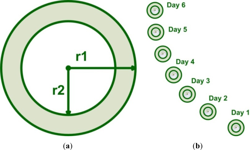
Pixels close to the hurricane center are usually covered by clouds, making it impossible to retrieve AOT with MODIS measurements. Thus, for this study, a unique technique was developed to select spatial coordinates to investigate aerosol retrievals as shown in
Table 2 around each hurricane. Two concentric circles with radii r1 and r2, as shown in
Figure 1(a), were drawn with a common center. These circles were drawn to be approximately at the hurricane eye. The spatial regions for this analysis were chosen between the two concentric circles called an annulus. The concentric circle annulus thickness can be adjusted by varying the radii r1 and r2. In this study r1 and r2 were selected as 8 and 5 degrees respectively to produce a ring with 3 degrees annulus size. The selected region is far away from the center of the hurricane, but still around the hurricane edge, and can generate enough valid remote sensing measurements for analysis.
The phenomena being investigated are three-dimensional in case of the variables such as Relative Humidity and Temperature where data is available between sea level and top of the atmosphere (between 100 to 1,000 mb). Vertical Shear and Wind are also three-dimensional phenomena. Although the MODIS sensor on both the Aqua and Terra satellites provides a measure of the vertically integrated dust concentration [
20], the vertical distribution of the dust frequency was not considered in this study. In this study we selected MODIS Atmospheric retrievals as two-dimension at seven wavelengths (0.47, 0.56, 0.65, 0.86, 1.24, 1.64, and 2.13 μm), therefore, circles were used instead of spheres. Therefore, for this investigation of aerosol, retrievals around a hurricane that involves “concentric circles” with the hurricane eye is appropriate.
We investigated whether the 3 to 4 degrees of annulus size would be an appropriate spatial coordinate selection process because aerosol parameters were retrieved around each hurricane by following the direction of motion of a hurricane. Since linear motion of a hurricane is very slow, for example a hurricane’s forward speed averages around 15–20 mph [
35], selecting a large annulus size would mostly overlap the spatial region while retrieval happens every day at 1,200 and 1,800 h. Again, selecting a narrow annulus size such as 1 to 2 degrees would introduce significant error while averaging the values within the annulus. Therefore, 3 degrees is the best selection for this study.
MODIS aerosol data at 0.55 μm was averaged in the vicinity of 1,200 and 1,800 h and associated with the corresponding SHIPS data at 1,200 and 1,800 for each day. This technique was employed on a spatial area for studying all 24 hurricanes between the day they formed and the day they dissipated. The center of the concentric circle corresponds to the approximate location of the hurricane core. The angle within this region was spaced out into 36 segments of 10° each. Data for each 10° segment was retrieved and averaged resulting 36 data points at a particular time and date. The readings from these 36 segments were then further averaged to present a final average to demonstrate the values between 0° and 360°. For this analysis, this concentric circles center was programmed to move with the hurricane center for 1,200 and 1,800 h.
Aerosol retrieval variables (
Table 2) were retrieved around each hurricane by following the direction of motion of a hurricane as illustrated in
Figure 1(b). The response variables “Future Difference (FD) or Intensity Change” has been calculated based on the following formula: FD
future = VMAX
future − VMAX
current, for example, FD
06 = VMAX
06 − VMAX
current, where VMAX is the maximum 1-min wind speed. Similarly, FD
12, FD
18, FD
24, FD
30, FD
36, FD
42 and FD
48 are calculated. We started our analysis by combining the 49 SHIPS parameters from DeMaria
et al. [
22–
24] with the 7 aerosol retrievals as shown in
Table 2. Correlation analysis was performed for the intensity change lead time at 06, 12, 18, 24, 30, 36, 42 and 48 h (which are basically the eight response variables between FD
06 and FD
48). For each FD
future set, correlation analysis will be performed with each of the 56 variables to determine the correlation coefficient (cc) between each variable and the FD
future. Variables having small correlation (|cc| < 0.165) were filtered out. These correlation based filtering create the first set of predictor, Predictor_1 which comprised 31 variables.
As the second step of data reduction, PCA is carried out on selected variable groups. The reduction of variables for each group by PCA is described in
Table 3. Prior to carrying out PCA on the five categories, variables were normalized to avoid skewness caused by units of the variables.
PCA is known as a variable reduction procedure and is useful when variables are significantly correlated. In each group, the variables describe the same physical mechanisms. The numbers of some group variables were shrunk to a reduced number of principal components. Although the details may be different among variables, their overall trends are the same based on their values. Therefore, using PCA to identify a reduced number of variables in the same group is a natural step. In this case, AOT, MCO, CCNO variables reduced to Aero-PC1 and Aero-PC2 for the Aerosol group and presented in the combination as Predictor_2. Similarly, for the Wind group, V20C U200 U20C TWAC TWXC are reduced to Wind-PC1 Wind-PC2 Wind-PC3 and presented as a combination of Predictor_3.
There will be some loss of information when a variable reduction was performed, therefore, when this technique was applied we made sure to select group of variables which exhibit similar physical phenomena to minimize loss of information. We have analyzed MODIS aerosol retrievals and SHIPS parameters for 24 hurricanes spanning 7 hurricane seasons. By combining MODIS and SHIPS data, 56 variables were compiled and selected as predictors. Variable reduction from 56 to 31 was performed via correlation coefficients. Among these 31 variables, some are highly correlated or “redundant” with one another. For example, Sea Surface Temperature, Air Temperature and Ocean depth of the (20 and 26 °C) isotherm for the Temperature group are usually very strongly correlated. Therefore, one or two of these variables or the combination of the variables (potentially for a newly defined, more representative variable) could be used as a substitution for all the others. For our study we selected the variable which is most likely to be the direct cause of categorical response and relevant to the hurricane intensity studies and of course highly correlated.
Identification and comparison of the impact of our approach on uncorrelated and correlated variables described in
Table 4 by considering, for example, Aerosol and Temperature components. Among the original set of Aerosol variables (AOT AFBO BRBO MRO MCO ERO CCNO) only (AOT MCO CCNO) were highly correlated. We have excluded (AFBO BRBO MRO ERO) variables because they were not correlated as highly as (AOT MCO CCNO). Similarly, the original temperature set of variables was (E000 EPOS EPSS T000 RD26 T150 SST T250 T200 RD20 ENEG ENSS) and only (SST T250 T200 RD20 ENEG ENSS) were highly correlated. Uncorrelated variables (E000 EPOS EPSS T000 RD26 T150) were excluded from this analysis. For comparison we performed PCA on both correlated and uncorrelated variables followed by Multiple Linear Regression (MLR) by the Predictor_2 and Predictor_6 at FD48 and presented in the
Table 4.
When comparing the results we see for Predictor_2 and Predictor_6, R2, Adjusted R2 and F Values had decreased for uncorrelated case while RMSE had creased increased. This illustrated that uncorrelated variables had lost more information than the correlated variables.
For the Relative Humidity group, RH-PC1 RH-PC2 principal components were extracted from the variables RHLO RHMD R000 and presented as Predictor_4. Predictor_5 and Predictor_6 were presented similarly for the Shear and Temperature groups. For each predictor the combination of variables along with the principal components are shown in
Table 5. The PEFC REFC Z850 PENC MSLP PSLV was excluded from PCA because they described diverse physical processes. The PCA technique can only produce outcomes with very limited benefits from such a data set.
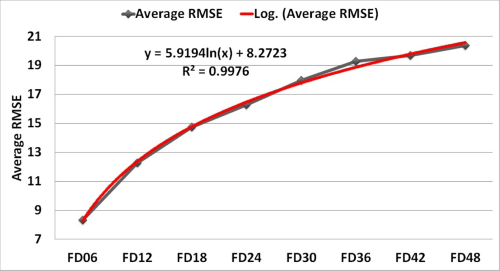
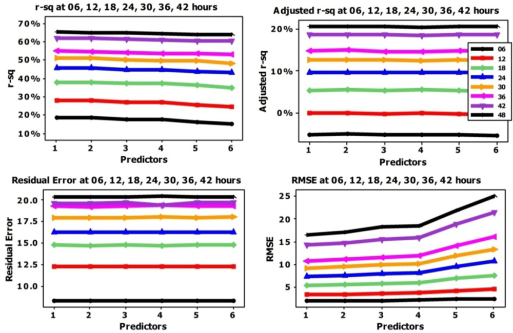
The average RMSE for the six Predictors for 06, 12, 18, 24, 30, 36, 42 and 48 h was found to be 8.33, 12.28, 14.76, 16.27, 17.96, 19.28, 19.69 and 20.38 respectively as illustrated in
Figure 2. The RED line is the logarithmic fit for the eight data points showing significant R
2 value. The variation among the Predictors RMSE varied between 0.01 through 0.05. This small variation suggests that reducing the number of variables did not change the core physical information. Therefore, the same phenomena can be explained by the reduction of a variable.
4. Results and Discussion
As shown in
Table 6 PCA for AOT, MCO and CCNO the cumulative results explain the variability for the first two components as 80.4% and 98.4%. For V20C U200 U20C TWAC TWXC, the top three principal components demonstrate a variability of 52.8%, 82.8% and 98.4%. When PCA was performed on RHLO RHMD R000, we have the cumulative variability for the first two components as 66.67% and 95.20%. PCA for SDDC SHDC SHGC SHRD SHRG SHRS SHTD SHTS gives variability for the four components as 50.7%, 72.0%, 81.4% and 88.8%. For SST T250 T200 RD20 ENEG ENSS, PCA results give variability for the first three components as 58.5%, 76.1% and 91.2%.
Dimensionality reduction infers loss of information; therefore, the goal is to preserve as much information as possible by minimizing difference between the higher (original) and lower dimensional variables representation. One of the commonly used methods to determine lower dimensional variables is the principal component analysis (PCA), in which the principal components, linear combination of the originals, ranked based on the contribution to the total variance, are chosen as new variables. The first few new variables are responsible for interpreting most of the physical phenomena described by the original variables that have been reduced.
Two Aerosol principal components explain 98.4% (loss = 1.6%) variability when variable reduction happened from three to two. For Wind, five variables were reduced to three principal components which resulted in a cumulative variability of 98.4% (loss = 1.6%). When PCA was performed on three Relative Humidity variables, it gave us cumulative variability for the two principal components as 95.20% (loss = 4.8%). PCA for eight Shear variables gives variability for the four reduced components as 88.8% (loss = 11.2%). Six Temperature variables were reduced to three components with 91.2% (loss = 8.8%) cumulative variability.
Reducing the variables does not always lead to a better result, but it is expected that the result should be comparable to that with original variables. Reduction of variables removes irrelevant features and dampens noise; it also leads to more comprehensible model because the model involves fewer variables [
36].
For the aerosol category the first two components have the proportionality of 0.80 and 0.18 respectively. Most of the weight is on the Aero-PC1 component which is about four times larger than Aero-PC2. For the Wind category, the first component is less than two times the second component and over three times larger than the third component. The proportion for Humidity shows that the first component is twice as large as the second component. Shear has a proportion of about 51% for the first component. The first component of the temperature has about 59% weight. When comparing the first component of the Aerosol, Wind, Relative Humidity, Shear and Temperature we found that aerosol had the highest proportion followed by Humidity, Temperature, Wind and Shear. Therefore, aerosol might have some influence based on the first component comparison.
In
Table 6, the cumulative variability percentage for each extracted component is presented, where the cumulative % threshold was set at 88%.
MLR technique was applied for the model forecast lead time of 06, 12, 18, 24, 30, 36, 42 and 48 h. For each FD
future, six predictor sets (Predictore_1 through Predictor_6) variables were analyzed.
Table 7 shows the common measures of MLR, and from this table, we can see for FD06, R
2 varied between 15.0% and 18.8% which is about 25.3% variation. For FD12, R
2 varied between 24.4% and 27.8% which is about 22.7% variation. The smallest variation for FD48 is 9.3% between the highest and lowest values.
Let us select FD48 as the response and explanatory variables as Original set of 56, Predictor_1 as 31 and Predictor_6 as 20. For the Original variables, 55 degrees of freedom (DF) provide us with RMSE = 19.47, R2= 71.1%, R2 (adj) = 64.5%, F = 10.72 and P = 0.000. For Predictor_1, DF = 30, RMSE = 20.38 R2= 65.1%, R2 (adj) = 61.1%, F = 16.46 and P = 0.000. For Predictor_6, DF = 19 RMSE = 20.36 R2 = 63.7% R2 (adj) = 61.2% F = 25.02 P = 0.000. One interesting finding is that the adjusted R2 with 20 variables is larger (or equal to) the corresponding value with 31 variables. At least in this special case, reducing the number of variables does not reduce the effectiveness of the MLR model but increases the efficiency.
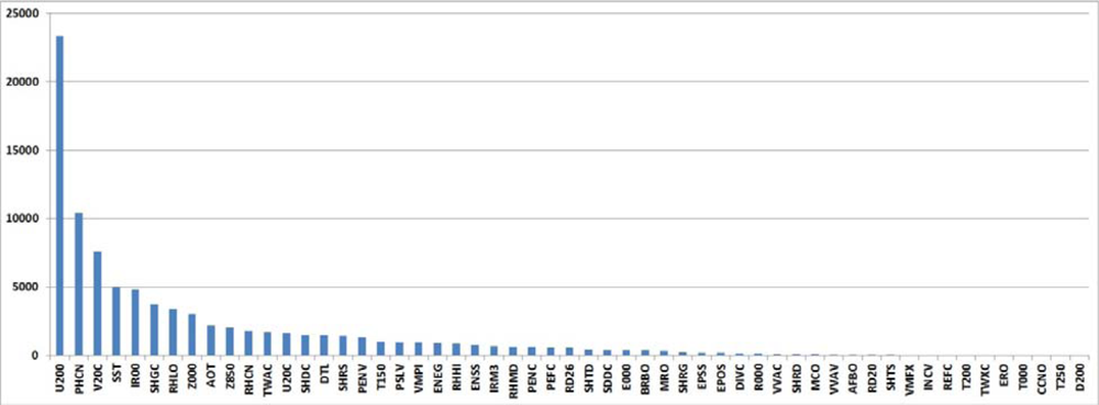
Figures 3–
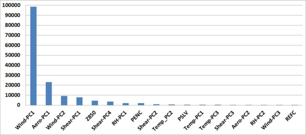
5 illustrates the contribution factor based on the MLR performed between FD48 and the 55 original variables (MSLP was taken out from the analysis because its contributing factor was high), Predfictor_1 of 31 variables and Predictor_6 of 20 variables respectively. We found aerosol, wind, humidity, shear and temperature all contributing factors in the regression equation. Based on
Figure 5, the Predictor_6 plot, the ranking for the contribution was found as (1) Wind, (2) Aerosols, (3) Shear, (4) Relative Humidity, and (5) Temperature components. Further breakdown, as in
Figure 4, showed that U200 and PHCN has the highest contribution then V20C followed by SST.
Figure 3 tells us about the effect of the SHIPS and MODIS variables used on the FD48. R
2 = 71.1% indicating that about 71% of the variation in FD48 can be accounted for by the 56 predictors. Based on the results of the Sequential Sum of Squares we can see components such as zonal winds, estimated ocean heat content and sea surface components are the greatest contributors to the MLR. This is also true for the intensity changes at 06, 12, 18, 24, 30, 36 and 42 h.
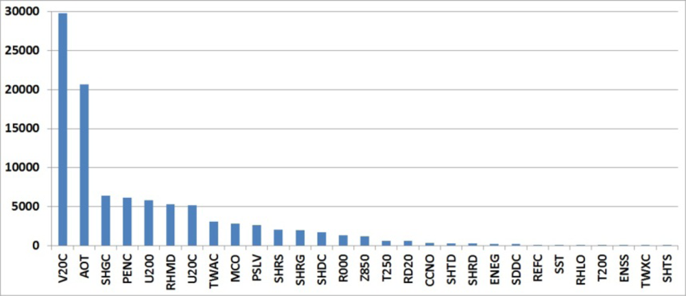
In
Figure 4, R
2 = 65.1% indicating that about 65% of the variation in FD48 can be accounted for by the 31 explanatory variables. The contribution factor in this case is mainly governed by the same variables as shown in
Figure 4 except we see Aerosol Optical Thickness (AOT) and relative humidity are playing significant roles as well. We also see Shear and Eddy play important roles in the case of Predictor_1.
The effect of the SHIPS and MODIS variables used on the FD48 as illustrated in
Figure 5, R
2 = 63.7% indicating that about 64% of the variation in FD48 can be accounted for by the 20 explanatory variables. The contribution factor in this case is governed by tangential and zonal wind in addition to AOT and RH.
Figure 6 shows the R
2 and adjusted R
2 values along with the RMSE and the Residual Errors for the MLR performed between the eight response variables and six predictor sets.
At 48 h forecast intervals as in
Figure 6, R
2, adjusted R
2 and RMSE are the largest and at 06 h, the smallest was recorded. The range of values of R
2, adjusted R
2 and RMSE between 06 and 48 h for Predictor_6 were found to be (15.0% and 63.7%), (9.1% and 61.2%), (8.35 and 25.02) and (69.64 and 415.0) respectively. The RMSE and Residual errors found negligible for all six predictors. However, significant R
2 values were found to be larger when considering the 42 and 48 h lead time for longer forecast intervals. This may be due to the results of discretization of the intensity of values as per DeMaria
et al. [
22,
23] and the regressions for the shorter forecast intervals may have been exposed to some noise [
22,
23].
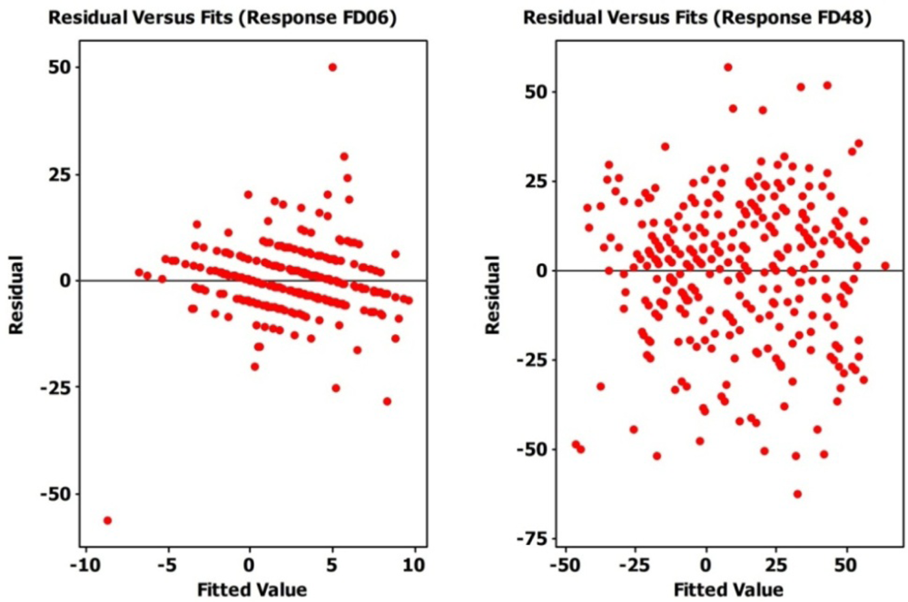
In
Figure 7 “Residuals
vs. fits” are presented to show the residuals vs. the fitted values at FD06 and FD48. Residuals varied between ±10 for FD06 whereas for FD48 its ±50 and FD06 has lesser outlier than FD48.
In addition, for this study MODIS Aerosol Retrievals were averaged, therefore, it is important to articulate the statistical uncertainty for the three variables used in the Aerosol PCA. For example, the quoted uncertainties for Fabian 2003 found for AOT (0.23 ± 0.02), MCO (15.54 ± 1.89) and CCNO (3.98 ± 0.781) × 108 when 95% confidence interval was considered.
5. Conclusions
By combining MODIS and SHIPS data, 56 variables were compiled and selected as predictors for this study. Variable reduction from 56 to 31 was performed via correlation coefficients (cc) followed by Principal Component Analysis (PCA) extraction techniques to further reduce these 31 variables to 20. Among the 31 variables, PCA candidates were selected for the variables describing the same physical mechanism and the PCA procedure reduces the numbers from 3–8 to 1–4 for each group of variables. Five categories: wind, aerosols, shear, relative humidity, and temperature components were established by reducing 56 variables to 20. Aerosol, wind, humidity, shear and temperature are all contributing factors in the regression equation with the ranking for the contribution found to be (1) Wind, (2) Aerosols, (3) Shear, (4) Relative Humidity, and (5) Temperature components. Indicating that aerosols predictor surpass the other predictors especially shear. However, from a dynamics point of view, it is impossible for aerosol to be more important than shear and temperature. The aerosol rank preceded the shear, which could be because our sample size was too small (306 data points) when compared to the original SHIPS dataset (over 6,000 data points) and inadvertently the value ranges of shear and temperature are not large. As a result, the limited variance in those parameters makes it is difficult to demonstrate the importance of those parameters. This is practically similar to a study with other parameter values being controlled. When the coefficient of variations (cv) was calculated we found cv for AOT 40.29%, Wind 37.61%, Shear 35.50%, SST 3.65% and Relative Humidity (RH) 6.8%. SST and RH cv values are so low that we can consider the experiment to be controlled at a specific value. In the same sense, it is not surprising to that AOT was the second dominated factor in this study because AOT are of the largest variability. When MLR is performed on all 56 variables (without any variable reduction) as illustrated in
Figure 3, interestingly, we see that aerosol is ranked in the last place. The original parameter describing aerosol effects are not a good choice. The linear combination of the original variables gives a much better description because of the much higher variance in the derived variable. As a result, although the AOT role is not among the first few parameters in the MLR model with all variables, the combined aerosol parameter plays a dominant role in the limited model.
There are plenty of benefits for overcoming the curse of dimensionality. Original variables may demonstrate better results but the reduced variables gave similar results with much lower dimensionality and improved efficiency. For computational purposes, improved efficiency is much more important than highly precise results.
One interesting finding is that the adjusted R2 with Predictor_6, 20 variables is larger than (or equal to) the corresponding value with Predictor_1 of 31 variables. At least in this special case, reducing the number of variables does not reduce the effectiveness of the MLR model but increases the efficiency.
The variation among the Predictors RMSE varied between 0.01 through 0.05. This implies that reducing the number of variables did not change the core physical information because variation is from the mean for all sets of predictors and very small. Therefore, the same phenomena can be explained by the reduction of the variable. R2 values were found to be larger when considering the 42 and 48 h lead time. R2, adjusted R2, RMSE and residual error among Predictor 1 through 6 was negligible. The RMSE and residual errors difference among the six predictor groups were found to be negligible.


