Article

Exploration of Loggerhead Shrike Habitats in Grassland National Park of Canada Based on in Situ Measurements and Satellite-Derived Adjusted Transformed Soil-Adjusted Vegetation Index (ATSAVI)

1
Department of Geography and Planning, University of Saskatchewan, Saskatoon, SK S7N5C8, Canada
2
Department of Geography, University of Toronto Mississauga, Mississauga, ON L5L1C6, Canada
*
Author to whom correspondence should be addressed.
Remote Sens. 2013, 5(1), 432-453; https://doi.org/10.3390/rs5010432
Submission received: 3 December 2012 / Revised: 10 January 2013 / Accepted: 14 January 2013 / Published: 21 January 2013

Abstract

:
The population of loggerhead shrike (Lanius ludovicianus excubutirudes) in Grassland National Park of Canada (GNPC) has undergone a severe decline due to habitat loss and limitation. Shrike habitat availability is highly impacted by the biophysical characteristics of grassland landscapes. This study was conducted in the west block of GNPC. The overall purpose was to extract important biophysical and topographical variables from both SPOT satellite imagery and in situ measurements. Statistical analysis including Analysis of Variance (ANOVA), measuring Coefficient Variation (CV), and regression analysis were applied to these variables obtained from both imagery and in situ measurement. Vegetation spatial variation and heterogeneity among active, inactive and control nesting sites at 20 m × 20 m, 60 m × 60 m and 100 m × 100 m scales were investigated. Results indicated that shrikes prefer to nest in open areas with scattered shrubs, particularly thick or thorny species of smaller size, to discourage mammalian predators. The most important topographical characteristic is that active sites are located far away from roads at higher elevation. Vegetation index was identified as a good indicator of vegetation characteristics for shrike habitats due to its significant relation to most relevant biophysical factors. Spatial variation analysis showed that at all spatial scales, active sites have the lowest vegetation abundance and the highest heterogeneity among the three types of nesting sites. For all shrike habitat types, vegetation abundance decreases with increasing spatial scales while habitat heterogeneity increases with increasing spatial scales. This research also indicated that suitable shrike habitat for GNPC can be mapped using a logistical model with ATSAVI and dead material in shrub canopy as the independent variables.

1. Introduction

The loggerhead shrike (Lanius ludovicianus excubutirudes), an open country bird, is widely distributed in North America from southern Canada to central Mexico [13]. However, loggerhead shrike in North America has undergone a great reduction during the past 40 years, which can be found in a number of documented studies [47]. In 1971 when the United States’ National Audubon Society bluelist provided an early warning of the population decline, loggerhead shrike has been identified as an endangered species by many wildlife preservation institutions [8,9]. Inadequate reproduction, pesticide contamination, and habitat loss are considered as three possible factors that can cause the shrike abundance decline [3,6,7]. However, breeding habitat loss or limitation may be the most responsible for the shrike reduced survivorship in that the bird species continued to decline after the poisoning pesticides were forbidden in United States since 1970’s [2,7]. Habitat selection can impact the species population in two ways: food availability and safety (predation risk), which is influenced by both vertical structure and spatial scales of the landscape as well as the topographical characteristics [2,10].
A ten year assessment of habitat use in southern Alberta concluded that shrub cover and presence of tall grass structure was associated with loggerhead shrike occupied territories. Shrike population is mainly dependent upon two features of the grassland landscape: shrubs taller than 1.8 m for nesting and tall grass for foraging [2]. However, in the past decade, changed ownership and land use have resulted in increasing utilization for pasture and decreasing shrub densities both in shelter belts (forest area for agriculture protection) and in riparian zones [11,12]. These factors combined with a lack of good population data where shrikes persist contribute to their threatened status [12]. Therefore, to reduce habitat loss for effectively preserving the endangered loggerhead shrike, it is of significance to identify the biophysical and topographical characteristics of their habitat preference especially at different spatial scales. However, most traditional efforts focused on identifying habitat features based on limited information obtained from field surveys which are time-consuming, laborious and expensive. Although remote sensing data has been widely used to assess the density and dispersion of vegetation of loggerhead shrikes by correlating imagery derived biophysical variables with ground based measurements of shrike habitats [1315], relatively little attention has been paid to the spatial patterns and scale variation of shrike habitat preference.
The purpose of this study is to investigate the loggerhead shrike habitat preference in Grassland National Park of Canada (GNPC) by measuring the in situ biophysical variables from different vertical structures as well as the important topographic variables (distance from roads, and elevation). Vegetation indices (VI) derived from satellite imagery was analyzed to extract the spatial variation and heterogeneity information of shrike distinct habitat types. This is intended to improve upon the previous shrike information content by focusing on the scale variation in vegetation communities (shrub community and adjacent grassland community) that are known of relevance. This study can help understand the impacts of current management decisions as well as seek alternative solutions for protecting potential suitable habitats and recover the previous ones degraded by exotic invasions or disturbances.

2. Study Area

Grassland National Park of Canada (GNPC), in southwest Saskatchewan, Canada (49°10′37″N, 107°25′33″W) with an area of around 906.5 km2, is a typical mixed grassland in North America. GNPC is the first national park established in Canada to preserve a portion of the vast mixed-prairie grasslands and the remaining ecological diversity in this region. It consists of two discontinuous blocks named the east block and the west block. The present study was conducted in the west block which is larger than the East one (Figure 1).
GNP has a semiarid continental climate with the temperature ranging from −55 °C to +45 °C and an annual precipitation of around 300 to 330 mm. Four major soil orders, Chernozemic, Solonetzic, Regosolic and Gleysolic, exist within the park region with the grassland communities most commonly characterized with Chernozemic soil. The dominant vegetations are blue grama grass, needlegrass and silver sagebrush. The ground cover is composed of bare soil, mosses, lichens, shrub, forbs, green grasses, stones, and dead materials (standing dead and litter). Variations in climate, topography, and ground cover together contribute to the diversity of endangered or threatened flora and fauna in this part of the Canadian Prairies [16].
Recorded surveys in GNP suggest that the park supports a stable population of loggerhead shrikes, but a recent management plan adopted by the park for reintroduction of bison and fire practices may affect the availability of suitable habitat and the bird population (Figure 2). Shrub communities in GNPC occupy approximately 10% of the current park holdings and are perhaps the most heavily modified ecosystem in the park. Topographically limited to the riparian zone around ephemeral creeks and rivers, shrub communities have been affected by human altered hydrology along with the invasion of aggressive exotic plant species such as smooth brome (Bromus inermus). These changes will have an impact on loggerhead shrikes, yet we know little about the dynamics of these communities or the effects of management activities on their structures and stability.

3. Methods

3.1. Field Data Collection

Both field data and satellite imagery were used in this study. Field data was collected in the west block of GNP in June 2006 from 45 samples of three shrike habitat varieties according to nesting occurrence: 16 active nesting sites (currently maintained by a Loggerhead Shrike), 19 inactive sites (previous nests but unoccupied in the most recent survey), and 10 control sites (non-nesting areas) (Figure 3).
All of the sites were relied on Andrew Didiuk (Environment Canada, Canadian Wildlife Service) survey of Loggerhead Shrike nests in 2004 for baseline locations [17]. The geographic coordinates of the 45 points selected from the surveyed sites were recorded by GPS in order to accurately locate the corresponding points in the satellite imagery. Based on a stratified random sampling design, a square-shaped 10,000 m2 (100 m × 100 m) sample area was set for each point with two 100 m transects crossed and extended in each cardinal direction (North, South, East, West) (Figure 4). We measured the in situ data (LAI, hyperspectral reflectance, biomass estimation, vertical structure, and Daubenmire cover) within a quadrat (50 cm × 20 cm) placed on one side of the transect at 20 m intervals. LAI was measured using a LAI-2000 Plant Canopy Analyzer (LI-COR Inc., Lincoln, NE, USA) based on the radiative transfer theory of canopy light interception calculated by one above-canopy reading and six below-canopy readings. Canopy reflectance used for calculating a vegetation index was collected using an ASD spectroradiometer (Boulder, CO, USA) within noon hours (from 10:30 am to 3:00 pm) on sunny days. The details regarding VI calculation can be found in later sections of this paper. Ground plant cover percentage was visually estimated by the observer. In addition, distances of different sites to roads and site elevation were also measured to provide topological information for loggerhead habitat investigation. For biomass estimation, in each site the vegetation was clipped to ground level and litter lightly raked using a quadrat of 50 cm × 20 cm (as stipulated by the Park). The clipped vegetation was stored in labeled bags (date, site, and plot) and later sorted into the different types (shrub, grass, forbs, and dead material) and weighed to estimate the live weight. Finally, they were oven dried at a temperature of 60 °C for 48 hours to get the dry weight. All in situ measurements from each habitat variety were averaged to represent the characteristic of that nesting category (Table 1).

3.2. Satellite Imagery Pre-Processing and Biophysical Variables Extraction

Multispectral SPOT 4 satellite imagery with 20 m spatial resolution acquired on 28 June 2006 was purchased for the study area, which was consistent with the time of field measurement. Imagery preprocessing was conducted for geometric and radiometric corrections using PCI Geomatica software. First, the images geometric error was removed through rectification with another geo-coded image (geocorrected Landsat TM image with 20 m spatial resolution for GNPC acquired on 14 July 2005) [18]. The correction accuracy is better than 0.1 Root Mean Square (RMS). Based on the dark object subtraction algorithm, atmospheric and radiometric correction was conducted to convert the original digital number (DN) values to the surface scaled reflectance [19]. Theoretically, it is better to perform first the radiometric corrections and then the geometric correction to avoid the modification of digital number (DN) values of pixels. However, we checked the results of different procedures and found that the results were almost similar. Therefore, the original pre-processed results were kept in this research. In order to analyze the spatial variation and heterogeneity of different habitat categories, Adjusted Transformed Soil Adjusted Vegetation Index (ATSAVI) was retrieved from the surface scaled reflectance based on the equation shown in Table 2[20]. Since ρ800 and ρ670 represent the NIR band and Red band respectively, we used the in situ reflectance in the exact narrow wavelengths to calculate ATSAVI. For SPOT data, band 3 (840 nm) and band 2 (650 nm) were applied as the NIR and Red bands to derive the image-based ATSAVI. It is difficult to measure in situ reflectance using quadrats at different spatial scales, so we used averaged image pixels for calculating ATSAVI for active, inactive and control sample sites at three spatial scales of 20 m × 20 m, 60 m ×60 m and 100 m ×100 m. 20 m ×20 m scale was calculated based on one pixel value while 60 m × 60 m were based on the average of 3 × 3 pixel values and 100 m × 100 m scale were based on the average of 5 × 5 pixel values (Figures 57, Table 3). Figures 57 show the difference of spectral reflectance among three types of habitat sites. The rectangle box of pixels shows the three pixel matrices (5 pixels × 5 pixels, 3 pixels × 3 pixels, 1 pixel × 1 pixel) which represent three spatial scales (100 m × 100 m, 60 m × 60 m, 20 m × 20 m) because one pixel is in the size of 20 m × 20 m. One small square box is one pixel zoomed in from the habitat sites in the SPOT image. These matrices can show the author what spatial scales were adopted. The grayscale color of pixels is an important element of image interpretation which is usually referred to as tone. The amount of reflected energy collected from the objects can be quantified by the degree of brightness or darkness. The greater energy reflected, the whiter the pixel of the surface target. Conversely, the less reflected energy, the darker the object pixel. Therefore, the gradual change from highest reflectance to lowest reflectance can be characterized by the tone change ranging from bright white to dark black. In these three figures, we can see that the tone of pixel patches is different for three types of habitat sites at three spatial scales. This is part of our methodological basis for this research.

3.3. Statistically Analyses

Both in situ and satellite imagery derived variables were statistically analyzed to extract the characteristics of different habitat categories. The homogeneity of variance criteria can be met because all significance values derived by Levene Statistic test are over 0.05. This indicates the equality of variances in different samples due to the acceptance of the null hypothesis that the population variances are equal. Then Analysis of Variance (ANOVA) was applied to the measured biophysical and topographical variables to detect the difference among active, inactive, and control nesting sites at a P-value of 0.10. A parametric analysis was conducted to found that the datasets can meet the criteria for applying ANOVA. Since the ANOVA results can only detect whether or not a difference exists, the Scheffe post-hoc test was chosen for its relatively conservative ability to determine exactly which site types differed significantly from one another. The results allow identification of some of the most relevant biophysical and topographical factors that significantly affect the habitat suitability. To determine the VI in estimating significant vegetation habitat characteristics, the correlation coefficients between ATSAVI and in measured vegetation variables were computed.
To detect the scale effect on different habitat categories, ATSAVI was compared at three scales to extract the spatial variation of vegetation distribution. ANOVA and the Scheffe post-hoc test were applied to identify the most different habitat types significantly affected by scale variation. According to the averaged coefficient of variance (CV) of ATSAVI within each 3 × 3 pixel matrix and 5 × 5 pixel matrix for each habitat category, the heterogeneity difference affected by scale variation was detected among three habitat sites.

3.4. Simulating Suitable Shrike Habitat Using Logistic Regression Model

A variety of analytical techniques have been used to investigate the relationship of wildlife habitat and environment [2226]. These include logistic regression [22], discriminate analysis [23], canonical correlation analysis [24], supervised non-parametric classifiers [25], and neural networks [26]. The most common analysis to define habitat suitability, which shows only the presence, is logistic regression.
For this purpose, a General Linear Model was developed by using presence-absence logistic regression design. This statistical analysis is especially helpful when presence has to be compared with absence (binary). At the same time, the outcomes show us how much a factor is significant in terms of nesting occurrence. Binary logistic regression has also been used to classify observations into one of two categories, and it may give fewer classification errors than discriminant analysis for some cases. Two types of environmental factors (biophysical and topographical) were the model predictors. Finally, a variety of statistical tests can be applied in order to assess how well the models describe the data. In this study, four tests (Pearson, Psuedo R2, predicted correct percentage, and Hosmer-Lemenshow) were used. The Hosmer-Lemenshow test assesses the fit of the model by comparing the observed and expected frequencies. The estimated probabilities are grouped from lowest to highest, and then the Chi Square statistic is calculated to determine if the observed and expected frequencies are significantly different. When the Hosmer-Lemenshow test is significant, it means that the observed counts and those predicted by the model are not close and the model does not describe the data well, and vice versa.

4. Results and Discussion

4.1. Measured Vegetation Characteristics for Different Habitat Categories

Our field survey found that 
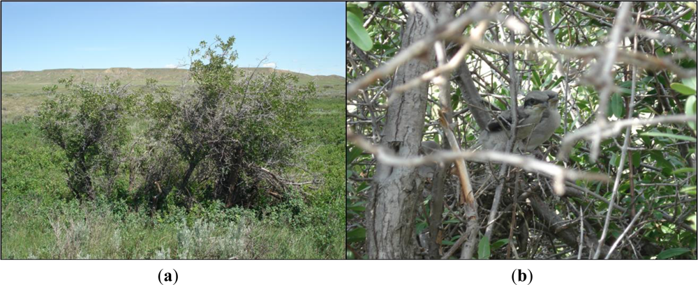
loggerhead shrikes prefer tall shrubs, especially thorny buffalo berry (Sheperdia argentea) for nest locations, because thorny species most likely discourage mammalian predators. This is consistent with the results in a previous study by [
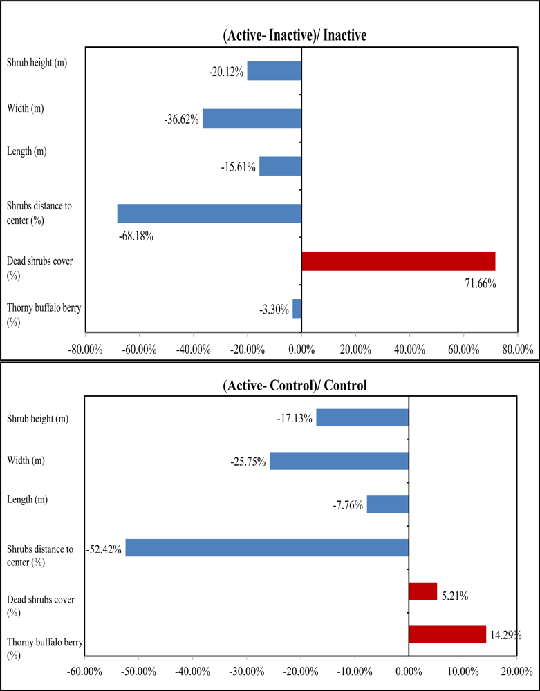
2]. Data analysis for the overstory showed that thorny buffalo berry occupies around 88% of tall shrubs in active sites, 91% in inactive sites, and 77% in control sites (
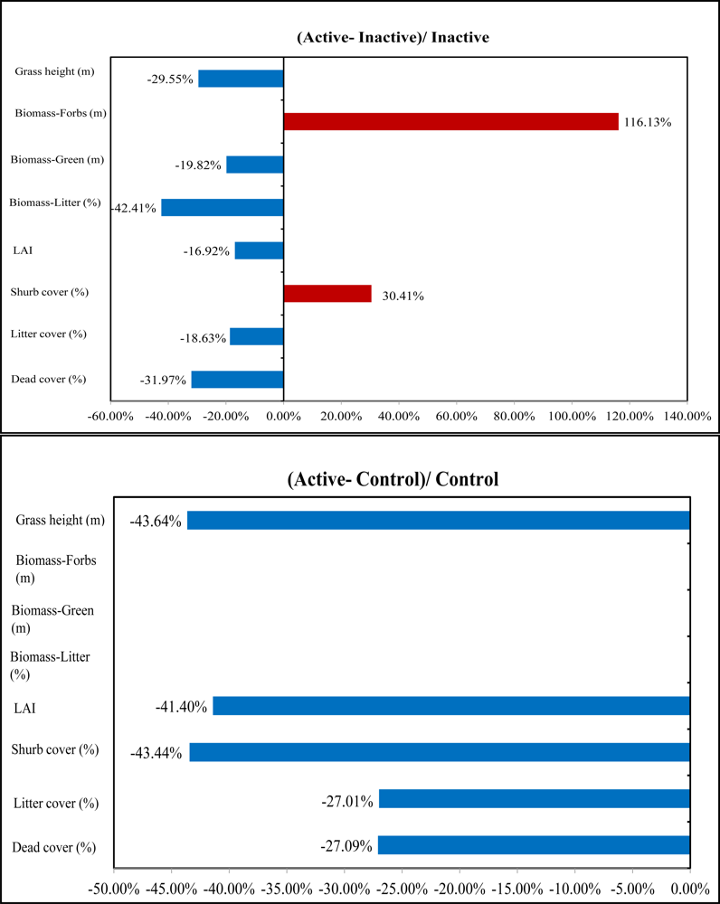
Table 1). The mean height of tall shrubs in active sites is 2.66 m, 20.12% shorter than that in inactive sites and 17.13% shorter than that in control sites (Figure 8). The ANOVA outcomes identified a significant difference in mean height existing between active and inactive sites with a P-value 0.06, indicating that shrikes may have a preference in tall shrubs with a height lower than 3 m for nesting. In addition, the active sites have the highest canopy cover of dead shrubs with 34.4% among the three habitat categories, 42% greater than that in inactive sties and 5% greater than in control sites (Figure 8). Therefore, shrike nesting sites are characterized by a high amount of dead materials, which was also supported by the significant difference between active and inactive sites in dead shrubs cover due to a P-value of 0.08 derived from ANOVA results. This is reasonable because shrikes can use dead branches to perch on while hunting for prey. Our analysis also revealed that dense thorny shrubs with less dead canopy in inactive sites are biophysical characteristics that may cause the site abandonment.
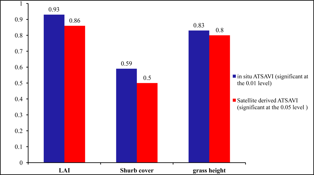
In the understory, active sites had the lowest LAI in comparison with the inactive and control sites. LAI has great potential in identifying nesting locations from non-nesting locations owing to the significant difference among the three habitat categories shown by the P values 0.01, 0.09, and 0.08. Therefore, the low LAI as well as less green biomass in active sites can strengthen the possibility that shrikes prefer nest locations with less grass productivity and more open spaces for easily identifying prey (Figure 9). Similar results can be also found in previous studies by [2,2729] which concluded that shrikes prefer open habitats characterized by vegetation of lower stature. In addition, the averaged grass height in active sites was 0.31 m; significantly shorter than that in other habitat types, which is consistent with the findings in the study by [30].

4.2. Measured Topographical Characteristics of Different Habitat Categories

Comparison of the topological characteristics among the three categories showed that shrikes’ occupied territories are farthest away from the roads at a higher elevation (Table 4). On average, active sites, inactive sites, and control sites were 2,227 m, 1,779 m and 1,315 m away from the road respectively. This indicated that shrikes prefer to locate their nests further from the roads to avoid jeopardizing the roadside habitats in predation, which is in accordance with the explanations by [29,31]. We also found that the elevation for active sites and for control sites is significantly different (P < 0.1). The active sites were, on average, at an elevation 4 m higher than inactive sites, and 6 m higher than control sites, possibly indicating that the high elevation of active sites can reduce predation rates and provide more food availability for shrikes in comparison with the other two sites.

4.3. Correlation of Vegetation Index and Biophysical Variables

Figure 10 showed that both the ground measured hyperspectral ATSAVI and imagery derived ATSAVI were significantly correlated with LAI, shrub cover, and grass height (P < 0.01 and <0.05), which demonstrated that this VI can be a good indicator of vegetation characteristics for loggerhead shrike habitats. ATSAVI was superior in estimating LAI and grass height compared to estimating shrub cover, which is consistent with a previous study in the same study area by [21]. By comparing the relationship between two types of ATSAVI and the selected biophysical variables, we also found that ATSAVI proved to be better at estimating vegetation characteristics at large spatial scales than at nesting scales due to the slightly higher correlation coefficients for the imagery derived ATSAVI.

4.4. Spatial variability of Vegetation for Different Habitat Categories

Control nesting sites showed significantly higher averaged ATSAVI than did the active and inactive sites at all three spatial scales (Table 5). This matches well with the fact that the active sites have higher dead shrub cover and lower green biomass derived from the in situ measurements analysis in Section 4.1. The difference between active and inactive sites is not significant because the period was only 2 years for the abandonment of the active sites. There may be some reason contributing to this transformation of these two habitat types, which we still have limited knowledge about to make specific an explanation. The spatial variation of ATSAVI indicated that vegetation abundance decreases as the spatial scales increase for all three types of habitat sites (Figure 11). The active sites have the most spatial heterogeneity at different scales, followed by inactive and then control sites. This means that areas of less spatial variation in vegetation may not be suitable for shrike nesting.

4.5. Spatial Heterogeneity of Vegetation for Different Habitat Categories

Heterogeneity is considered one of the most important indicators of prairie habitat. The grassland heterogeneity at different spatial scales can be contributed by various disturbances which increases wildlife biodiversity [32]. CV values in Table 6 showed vegetation heterogeneity declines from active sites, to inactive sites and then to control sites at both spatial scales. In particular control sites had significantly higher vegetation heterogeneity than did the active and inactive sites according to the ANOVA results with P values < 0.1. This indicated that shrike habitats are characterized by vegetation of high heterogeneity, which is consistent with the fact that shrikes prefer open nesting areas with scattered shrubs and higher dead material components for ease of foraging. As shown in Figure 12, the vegetation heterogeneity for all types of habitat categories increases with the spatial scales enlarged. It is possible that areas of moderate vegetation heterogeneity with a certain threshold are potential loggerhead shrike habitats. This can also be related with the fact that shrikes prefer smaller shrub sizes for nesting sites based on our in situ data analysis.

4.6. Suitable Shrike Habitat Modeling

The logistic regression coefficient, its standard error, and Wald test were shown in Table 7. The ratio of regression coefficient to standard error, squared, equals the Wald statistic. If the Wald statistic is significant (i.e., less than 0.05) then the parameter is useful to the model. For example, we can see that dead shrub canopy cover, shrub patch width, shrub patch height in Table 7(D, G, and H) resulted in a small Wald statistic, therefore, and these three variables might be useful to build the regression models.
The log likelihood, Pseudo R2 (Cox & Snell R2 and Nagelkerke R2), overall predicted correct, and Hosmer & Lemeshow test were presented in Table 7 to evaluate the models. R2 is comparable to R2 from ANOVA conducted on individual observations. The interpretation of the log likelihood and Pseudo R2 is: the less log likelihood, the higher R2, the more proportion of variation in the dependent variable accounted for by the independent variable or variables. In this case, 21% of variation in active or inactive of habitat sites was accounted for by an index of the dead shrub canopy cover. Comparing Table 7(D, G) we saw that the model with ‘dead shrub canopy cover’ accounted for 1% less of the variation in active and inactive than did the model with ‘shrub patches width’: the latter variable had a less log likelihood and, consequently, a greater Psuedo R2. Hosmer & Lemeshow Test is a goodness-of-fit test of the null hypothesis that the model adequately fits the data. If the null is true, the statistic should have an approximately chi-square distribution with the displayed degrees of freedom. If the significance of the test is small (i.e., less than 0.05) then the model does not adequately fit the data. Table 7(D) showed a close chi-square distribution (7.71) with the displayed degrees of freedom (7) and the significance (0.36) was greater than 0.05, then the model should fit the data. The overall predicted correct helped to assess the performance of the models.
Having obtained the results in Table 7(A–M), we conducted a multiple logistic regression analysis to determine how many different factors may be contributing to variation in the active habitat presence. We therefore ran another model, with the stepwise method to select the suitable independent variables, shown in Table 7(N). In this case, we saw that only two variables, ATSAVI and ‘Shrub dead canopy cover’, were selected to enter the model. The effect of each of the 2 variables was significant when controlling for the effect of the other. Note that the Pseudo R2 for the 2-variable model was higher compared to the Pseudo R2 for all other single variable models in Table 7(A–M). Thus, by including both ATSAVI and ‘Shrub dead canopy cover’ in the model, we are able to increase the Pseudo R2. We also examined the goodness of fit of the model in Table 7N and the results showed that no reason to reject the fit of the model, implying that the assumption made in logistic regression that residuals are binomially distributed was satisfied. The higher predicted correct in Table 7(N) (72%) showed the predicted probability of the model for nesting presence. Based on 
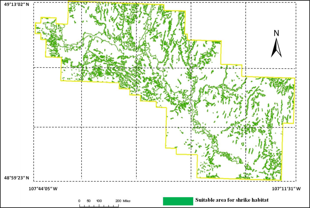
Table 7(N), the logistic model for suitable habitat mapping should be:
Y = 1 1 + e U , U = 0.73 + 0.127 Ds 12.6 × ATSAVI
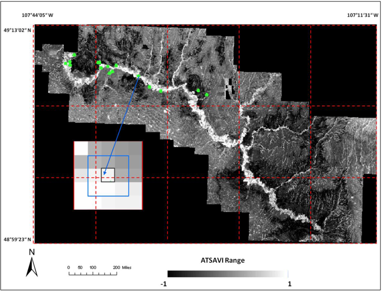
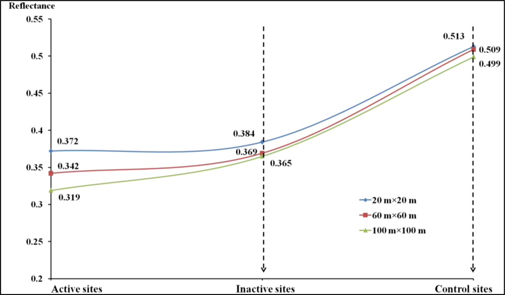
where Ds is dead material in tall shrub canopy. From above equation we can see that dead material in tall shrub canopy positive contribute to the shrike nest selection, and ATSAVI negatively contributes to the shrike nest selection. The ATSAVI is a greater negative contributor. This conclusion is consistent with the ATSAVI variation for different shrike habitat types which is shown in Figure 11. This model was applied to the SPOT image to derive the suitable habitat map for loggerhead shrike in GNPC (Figure 13). This map is a polygon file and can be easily used by Parks manager.

4.7. Uncertainties and Opportunities

As a preliminary research, our research suffers from several limitations and uncertainties. First, this study relied on Andrew Didiuk (Environment Canada, Canadian Wildlife Service) survey of loggerhead shrike nests in 2004 for baseline locations. Some shrike nests in GNPC might have not been accurately known, and the outliner or absence of records may result in inadequate exploration of shrike habitats. It is necessary to resurvey the study area in order to obtain more reliable sample data. Because the uncertainty arising from insufficient field datasets can lead to difficulty in validating the accuracy of habitat estimation. Other limiting factors include climate variation (temperature and precipitation), grazing, burning, and surrounding land-use activities (land conversions) that all might affect shrike abundance [3335].
Uncertainties can also be found in the field survey which covers quite a large area. In such situation, a gradient analysis method should have more potential than non-gradient approaches for accurately investigating habitat characteristics along the environmental gradient. Possible gradient methods contain PCA (principle component analysis), CA (Correspondence analysis), or DCA (detrended correspondence analysis). This can be promising a direction for our further research to improve the results.
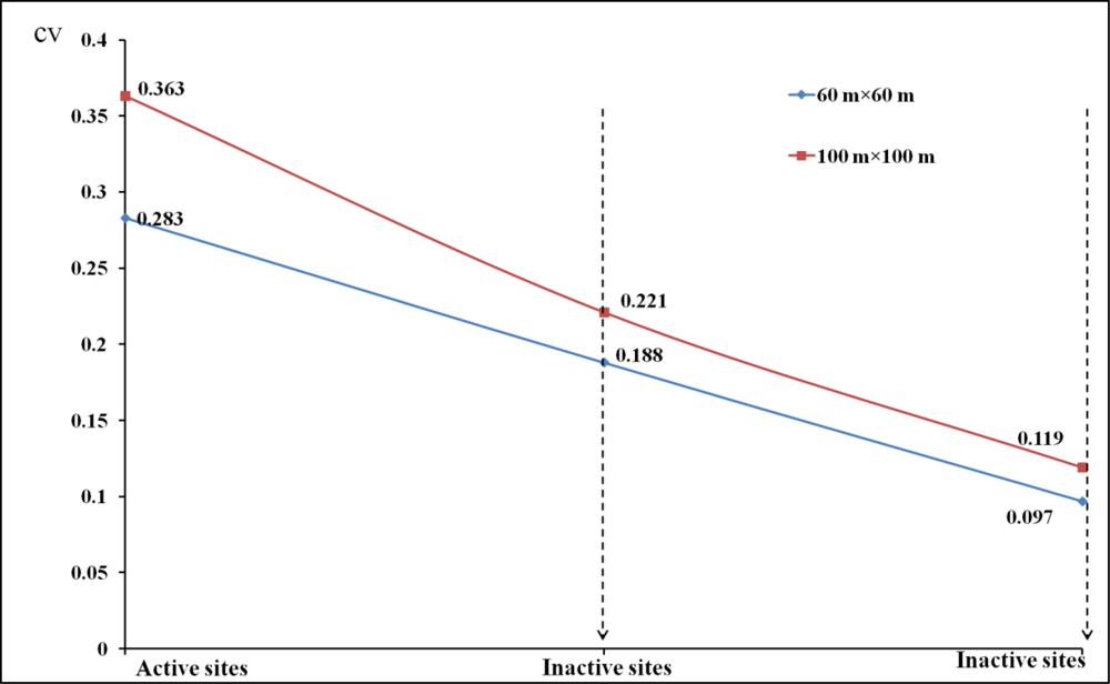
For remote sensing perspective of spatial heterogeneity, CV (Coefficient of variance) analysis can be further validated by measures such as landscape indices, fragmentation/connectivity measure, image segmentation, or image texture (e.g., GLCM-grey level co-occurrence matrix). However, due to the low spatial resolution of our available satellite imagery and the high level of heterogeneity of our study area, currently landscape indices and image segmentation performed poorly in this study for extracting meaningful information from shrike habitats.
Therefore, in order to eliminate or minimize the aforementioned uncertainties in our study, three important concerns need to be addressed in future research: (1) applying comprehensive census methods to detect more shrike nests in the study area; (2) investigating multiple habitat impacting factors.

5. Conclusions

Our study indicated that loggerhead shrikes prefer nesting sites characterized by tall shrubs (lower than 3 m), especially thorny buffalo berry which occupies approximately 88% of the total tall shrubs. In addition, the active sites have the highest dead shrub cover (34.4%) among three habitat categories, 42% greater than in inactive sties and 5% greater than in control sites. Dead materials are normally used by shrike to perch on while hunting for prey. Also, shrikes prefer nest locations with less grass productivity and more open spaces for easily identifying prey, due to the lowest LAI (average 1.67) observed in active sites compared to that in inactive (average 2.01) and control (average 2.85) sites. The most significant topographical characteristic of shrike territories found in this research is that shrike nesting sites are located further away from roads (over 2,000 m) at higher elevation.
Both ground measured and satellite imagery derived vegetation index (Adjusted Transformed Soil-Adjusted Vegetation Index-ATSAVI) is significantly related to most relevant biophysical factors: (Lear Area Index-LAI), shrub cover, and grass height with a correlation coefficient over 0.5 (P < 0.05). This proves that vegetation index can be a good indicator for shrike habitat characterization. Spatial variation analysis (at three scales: 20 m × 20 m, 60 m × 60 m and 100 m × 100 m) showed that for all spatial scales active sites have the lowest vegetation abundance (LAI: 0.372, 0.342, 0.319) and highest heterogeneity (Coefficient of Variance-CV: 0, 0.283, 0.363) among the three types of nesting sites. A logistic model can be used to spatially estimate habitat area for loggerhead shrike based on suitable independent variables (ATSAVI and shrub dead canopy cover) with a higher predicted probability (72%).
For suggestions to protect loggerhead shrike habitats in future park management, our findings demonstrated that it is necessary to preserve native grass and thorny shrub species within shrike’s breeding range. In areas with taller grass, grazing (introducing bison) might be able to provide suitably short vegetation for shrike foraging as well as for increasing shrike productivity [36,37]. However, a few areas of tall grass should be maintained within pastures as they can serve as food reserves for small mammals, which are potential shrike’s prey [2]. Since the loggerhead shrike prefers more open spaces, managing dense woody vegetation is highly recommended.

Acknowledgments

This research was supported by Parks Canada Funding (5P401-06-5007), NSERC, and ISTPCanada. The authors are grateful to the anonymous reviewers whose suggestions have been helpful in preparation of the manuscript. The authors also would like to acknowledge Jordon Steeg who helped to improve the English language of this manuscript.

References

  1. Burnside, F.L.; Shepherd, W. Population trends of the loggerhead shrike (Lanius Ludovicianus) in Arkansas. Proc. Ark. Acad. Sci 1985, 39, 25–28. [Google Scholar]
  2. Prescott, D.C.; Collister, D.M. Characteristics of occupied and unoccupied loggerhead shrike territories in southeastern Alberta. J. Wildl. Manag 1993, 57, 346–352. [Google Scholar]
  3. Brooks, B.L.; Temple, S.A. Dynamics of a loggerhead shrike population in Minnesota. Wilson Bull 1990, 102, 441–450. [Google Scholar]
  4. Bystrak, D.; Robbins, C.S. Bird population trends detected by the North American breeding bird survey. Pol. Ecol. Stud 1977, 3, 131–143. [Google Scholar]
  5. Hess, B.K. Summary of the status of shrikes in Delaware. Delmarva Ornitho 1980, 15, 8–9. [Google Scholar]
  6. Kridelbaugh, A.L. Population trend, breeding and wintering distribution of loggerhead shrikes Lanius ludovicianus in Missouri. Trans. Missouri Acad. Sci 1981, 15, 111–119. [Google Scholar]
  7. Gawlik, D.E.; Bildstein, K.L. Seasonal habitat use and abundance of loggerhead shrikes in South Carolina. J. Wildl. Manag 1993, 57, 352–357. [Google Scholar]
  8. National Audubon Society. Announcing the Blue List an “early warning system” for birds. Am. Birds 1971, 25, 948–949. [Google Scholar]
  9. Tyler, J.D. Nesting ecology of the loggerhead shrike in southwestern Oklahoma. Wilson Bull 1992, 104, 95–104. [Google Scholar]
  10. Chalfoun, A.D.; Martin, T.E. Assessments of habitat preferences and quality depend on spatial scale and metrics of fitness. J. Appl. Ecol 2007, 44, 983–992. [Google Scholar]
  11. Willms, W.D.; Dormaar, J.F.; Adams, B.W.; Douwes, H.E. Response of the mixed prairie to protection from grazing. J. Range Manag 2002, 55, 210–216. [Google Scholar]
  12. Bjorge, R.R.; Prescott, D.R.C. Population estimate and habitat associations of the loggerhead shrike, Lanius ludovicianus, in Southeastern Alberta. Can. Field Nat 1996, 110, 445–449. [Google Scholar]
  13. Jobin, B.T.; Grenier, M.; Laporte, P. Using satellite imagery to assess breeding habitat availability of the endangered loggerhead shrike in Quebec. Biodivers. Conserv 2005, 14, 81–95. [Google Scholar]
  14. Penniket, R. Aerial Photography Interpretation and Mapping for Silver Sagebrush, Final Summary Report; Parks Canada Agency: Calgary, AB, Canada, 2004. [Google Scholar]
  15. Guo, X.; Wilmshurst, J.F.; Zhang, C.; Sissons, R.; Fargey, P. Measuring Grassland Structure for Recovery of Grassland Species at Risk; Final Report 5P401–04–5002; University of Saskatchewan, Saskatoon: Saskatoon, SK, Canada, 2005. [Google Scholar]
  16. Li, Z.; Guo, X. A suitable vegetation index for quantifying temporal variation of leaf area index (LAI) in semiarid mixed grassland. Can. J. Remote Sens 2011, 36, 709–721. [Google Scholar]
  17. Didiuk, A. Prairie Loggerhead Shrike Habitat Assessments and Surveys on Federal Lands, Grasslands National Park, West Block and East Block 2003–2004. Unpublished Progress Report. 2005. [Google Scholar]
  18. Jensen, J.R. Introductory Digital Image Processing: A Remote Sensing Perspective, 3rd ed.; Pearson Prentice Hall: Upper Saddle River, NJ, USA, 2005. [Google Scholar]
  19. Chavez, P.S. An Improved dark-object subtraction technique for atmospheric scattering correction of multispectral data. Remote Sens. Environ 1988, 24, 459–479. [Google Scholar]
  20. Baret, F.; Guyot, G. Potentials and limits of vegetation indices for LAI and APAR assessment. Remote Sens. Environ 1991, 35, 161–173. [Google Scholar]
  21. He, Y.; Guo, X.; Wilmshurst, J. Studying mixed grassland ecosystems I: Suitable hyperspectral vegetation indices. Can. J. Remote Sens 2006, 32, 98–107. [Google Scholar]
  22. Wang, K.; Franklin, S.F.; Guo, X.; Collingwood, A.; Stenhouse, G.B.; Lowe, S. Comparison of Landsat multispectral and IRS panchromatic Imagery for landscape pattern analysis of grizzly bear habitat in agricultural areas of western Alberta. Can. J. Remote Sens 2010, 36, 36–47. [Google Scholar]
  23. Robinson, T.; Rogers, D.; Williams, B. Mapping tsetse habitat suitability in the common fly belt of Southern Africa using multivariate analysis of climate and remotely sensed vegetation data. Med. Vet. Entomol 1997, 11, 235–245. [Google Scholar]
  24. Carter, J.L.; Fend, S.V.; Kennelly, S.S. The relationships among three habitat scales and stream benthic invertebrate community structure. Freshw. Biol 1996, 35, 109–124. [Google Scholar]
  25. Ferguson, R.S. Detection and classification of muskox habitat on Banks Island, Northwest Territories, Canada, using Landsat Thematic Mapper data. Arctic 1991, 44, 66–74. [Google Scholar]
  26. Joy, M.K.; Death, R.G. Predictive modeling and spatial mapping of freshwater fish and decapod assemblages using GIS and neural networks. Freshw. Biol 2004, 49, 1036–1052. [Google Scholar]
  27. Stewart, R.E. Breeding Birds of North Dakota; Tri-College Center for Environmental Studies: Fargo, ND, USA, 1975. [Google Scholar]
  28. Brooks, B.L.; Temple, S.A. Dynamics of a loggerhead shrike population in Minnesota. Wilson Bull 1990, 102, 441–450. [Google Scholar]
  29. De Geus, D.W. Productivity and Habitat Preference of Loggerhead Shrikes Inhabiting Roadsides in a Midwestern Agroenvironment. Iowa State University, Ames, IA, USA, 1990. [Google Scholar]
  30. Yosef, R.; Grubb, T.C. Effect of vegetation height on hunting behavior and diet of loggerhead shrikes. Condor 1993, 95, 127–131. [Google Scholar]
  31. Crabtree, R.L.; Broome, L.S.; Wolfe, M.L. Effects of habitat characteristics on gadwall nest predation and nest-site selection. J. Wildl. Manag 1989, 53, 129–137. [Google Scholar]
  32. Guo, X.; Wilmshurst, J.; McCanny, S.; Fargey, P.; Richard, P. Measuring spatial and vertical heterogeneity of grasslands using remote sensing techniques. J. Environ. Inform 2004, 3, 24–32. [Google Scholar]
  33. Cleckner, H.L.; Allen, T.R.; Bellows, A.S. Remote sensing and modeling of mosquito abundance and habitats in Coastal Virginia, USA. Remote Sens 2011, 3, 2663–2681. [Google Scholar]
  34. Wondie, M.; Schneider, W.; Melesse, A.M.; Teketay, D. Spatial and temporal land cover changes in the Simen Mountains National Park, a world heritage site in Northwestern Ethiopia. Remote Sens 2011, 3, 752–766. [Google Scholar]
  35. Ndegwa Mundia, C.; Murayama, Y. Analysis of land use/cover changes and animal population dynamics in a wildlife sanctuary in East Africa. Remote Sens 2009, 1, 952–970. [Google Scholar]
  36. Hands, H.M.; Drobney, R.D.; Ryan, M.R. Status of the Loggerhead Shrike in the North Central US (Unpublished Report). 1989. [Google Scholar]
  37. Hellman, S.L. Breeding Habitat, for the Loggerhead Shrike (Lanius ludovicianus) in Southwestern Manitoba. 1994. [Google Scholar]
Figure 1. Study area (the west block of GNP).
Remotesensing 05 00432f1
Figure 2. Landscape and loggerhead shrike in the west block of GNP in 2006. (a) Thorny Buffalo berry for shrike habitats; (b) Physical look of loggerhead shrike.
Remotesensing 05 00432f2
Figure 3. Loggerhead shrike nesting sites for different habitat types in the west block of GNP in 2006.
Remotesensing 05 00432f3
Figure 4. Stratified random sampling design for field data collection.
Remotesensing 05 00432f4
Figure 5. ATSAVI for active sites at different spatial scales (20 m × 20 m, 60 m × 60 m and 100 m × 100 m).
Remotesensing 05 00432f5
Figure 6. ATSAVI for inactive sites at different spatial scales (20 m × 20 m, 60 m × 60 m and 100m × 100 m).
Remotesensing 05 00432f6
Figure 7. ATSAVI for control sites at different spatial scales (20 m × 20 m, 60 m × 60 m and 100 m × 100 m).
Remotesensing 05 00432f7
Figure 8. Relative difference of overstory characteristics among sites.
Remotesensing 05 00432f8
Figure 9. Relative differences of understory characteristics among sites.
Remotesensing 05 00432f9
Figure 10. The Correlation Coefficients between ATSAVI and significant vegetation variables.
Remotesensing 05 00432f10
Figure 11. Spatial variation of ATSAVI at three spatial scales for different habitat categories.
Remotesensing 05 00432f11
Figure 12. Spatial heterogeneity represented by CV for different habitat types.
Remotesensing 05 00432f12
Figure 13. The suitable shrike habitat mapping based on a logistic model for Loggerhead shrink in the west block of GNPC in 2006.
Remotesensing 05 00432f13
Table 1. Measured overstory and understory biophysical characteristics and significance results for different habitat sites.
Measured VariablesMeanSignificance

Active SitesInactive SitesControl SitesActive-ControlActive-InactiveControl-Inactive
Overstory
Thorny buffalo berry of tall shrubs (%)8891770.8610.49
Dead shrubs cover (%)34.3520.0132.6510.08*0.25
Shrub distance to center (m)5.416.9711.350.990.11
Length (m)6.547.757.09111
Width (m)3.986.285.360.710.09*1
Shrub height (m)2.663.333.210.280.06*1
Understory
Dead Cover (%)7.5111.0410.30.970.461
Litter cover (%)67.0682.4191.870.130.441
Shrub cover (%)24.5318.8143.370.02*0.950*
LAI1.672.012.850.01*0.09*0.08*
Biomass-Litter (g)25.7944.78N/AN/A0.3N/A
Biomass-Green(g)9.7512.16N/AN/A0.5N/A
Biomass-Forbs (g)1.340.62N/AN/A0.5N/A
Grass height (m)0.310.440.550.018*N/AN/A
*Small significance values (<0.1) indicate group differences.
Table 2. Biophysical VIs investigated in this study.
Vegetation Indices (VIs)EquationReference
Adjusted Transformed Soil-Adjusted Vegetation Index (ATSAVI) a ( ρ 800 a ρ 670 b ) a ρ 800 + ρ 670 a b + X ( 1 + a 2 ) , X = 0.08Baret and Guyot [19]
Note: The coefficients a (gain) and b (offset) in the equation for ATSAVI are derived from the NIR-Red rock-soil baseline. In our study area, a is 1.22 and b is 0.03 [21]. ρ, reflectance. When calculated VIs using satellite data, ρ800, ρ670 in the equation were ρNIR and ρRed, respectively.
Table 3. Control sites in the false color composite reflectance imagery of 28 June 2006.
Habitat SitesATSAVI (1 Pixel)ATSAVI(3 × 3 Pixels)ATSAVI (5 × 5 Pixels)
Active Sites
10.2580.2840.272
20.5010.4850.473
30.0540.1120.098
40.2170.1560.128
50.5760.5240.522
60.4630.3730.328
70.5030.4560.406
80.4480.4040.390
90.3270.3250.332
100.5390.4630.377
110.3470.3420.263
120.4960.4190.420
130.5410.4720.433
140.3160.2420.239
150.2420.2450.253
160.1210.1750.171
Inactive Sites
10.2010.1980.207
20.4550.4690.472
30.240.2240.240
40.3510.3070.309
50.2810.2900.317
60.5200.5330.529
70.5070.5110.505
80.4450.4780.465
90.4320.3270.298
100.5140.4340.422
110.5170.4680.459
120.4370.4230.397
130.2630.3040.307
140.4190.3980.380
150.5380.5220.527
160.0720.1440.165
170.2230.2150.200
180.5080.4450.432
190.3800.3250.307
Control Sites
10.5530.5140.477
20.5440.5180.509
30.6070.5530.529
40.3640.4090.422
50.5760.5700.548
60.4850.4950.496
70.3770.4390.451
80.5370.5370.526
90.5300.4910.474
100.5570.5610.557
Table 4. Measured topographical characteristics and ANOVA results for different habitat sites.
Measured VariablesStatistical VariablesActive SitesInactive SitesControl SitesSig.*
Active-InactiveActive-ControlInactive-Control
Distance to road (m)Mean2,2271,7791,3150.301.001.00
Elevation (m)Mean7797757730.240.430.02*
*Small significance values (<0.1) indicate group differences.
Table 5. Spatial variation of ATSAVI at three spatial scales for different habitat categories.
Habitat CategoriesStatistical VariablesActive SitesInactive SitesControl SitesSig.*
Active-InactiveActive-ControlInactive-Control
ATSAVI (20 m × 20 m)Mean0.3720.3840.5130.810.02*0.01*
ATSAVI (60 m × 60 m)Mean0.3420.3690.5090.520.00*0.00*
ATSAVI (100 m × 100 m)Mean0.3190.3650.4990.260.00*0.00*
*Small significance values (<0.1) indicate group differences.
Table 6. Heterogeneity of ATSAVI at three spatial scales for different habitat categories.
Habitat CategoriesAveraged CV for Pixels in Each SiteActive SitesInactive SitesControl SitesSig.*
Active-InactiveActive-ControlInactive-Control
ATSAVI (60 m×60 m)Mean CV0.2830.1880.0970.0810.003*0.024*
ATSAVI (100 m×100 m)Mean CV0.3630.2210.1190.0090.000*0.005*
*Small significance values (<0.1) indicate group differences.
Table 7. Logistic regression analysis of active/inactive sites in relation to habitat features. The independent variable is detection of habitat sites based on surveys. Simple logistic regression in relation to significant vegetation and topographical parameters (AM). Best multiple logistic regression model, and associated goodness-of-fit statistics (N).
Model EvaluationModel Summary
Log likelihoodPseudo R2Overall Predicted CorrectHosmer & Lemeshow
Cox& Snell R2Nagelkerke R2Chi-SquaredfSig.Cons.Coef.S.EWaldSig.
A) Independent variable: Distance to roads
45.710.030.0459%9.7280.29−0.750.000.000.940.33
B) Independent variable: SPOT4 ATSAVI
45.720.030.0459%7.2680.510.65−2.772.890.920.34
C) Independent variable: Thorny buffalo berry percentage
37.240.100.0152%2.6720.260.56−0.711.830.150.70
D) Independent variable: Dead shrub canopy cover
30.020.210.2865%7.7170.360.070.070.034.670.03
E) Independent variable: Shrub distance to center
29.440.220.3065%4.8270.681.13−0.130.082.700.10
F) Independent variable: Shrub patch length
35.130.030.0562%12.9570.070.84−0.120.130.860.35
G) Independent variable: Shrub patch width
29.660.220.2977%2.8770.902.67−0.550.274.050.04
H) Independent variable: Shrub patch height
30.500.190.2673%4.8670.684.73−1.610.893.280.07
I) Independent variable: Dead cover in understory
35.920.090.1250%4.6970.700.76−0.110.072.060.15
J) Independent variable: Litter cover in understory
36.910.060.0857%4.9070.671.18−0.020.011.640.20
K) Independent variable: Forb cover in understory
36.920.020.0252%4.1070.770.34−0.060.090.460.50
L) Independent variable: Shrub cover in understory
37.420.040.0654%7.6870.36−0.840.030.031.200.27
M) Independent variable: LAI
38.010.020.0350%10.9370.140.53−0.360.450.640.42
N) Best multiple logistic regression model: STEPWISE
23.190.370.4972%50.5460.540.73
ATSAVI−12.66.533.7390.05
Shrub Dead Canopy Cover0.1270.065.0560.02

