A Sequential Aerial Triangulation Algorithm for Real-time Georeferencing of Image Sequences Acquired by an Airborne Multi-Sensor System

Department of Geoinformatics, The University of Seoul, Seoulsiripdaero 163, Dongdaemun-gu, Seoul,Korea
*
Author to whom correspondence should be addressed.
Remote Sens. 2013, 5(1), 57-82; https://doi.org/10.3390/rs5010057
Submission received: 3 October 2012
/
Revised: 14 December 2012
/
Accepted: 17 December 2012
/
Published: 24 December 2012
Abstract
:Real-time image georeferencing is essential to the prompt generation of spatial information such as orthoimages from the image sequence acquired by an airborne multi-sensor system. It is mostly based on direct georeferencing using a GPS/INS system, but its accuracy is limited by the quality of the GPS/INS data. More accurate results can be acquired using traditional aerial triangulation (AT) combined with GPS/INS data, which can be performed only as a post-processing method due to intense computational requirements. In this study, we propose a sequential AT algorithm that can produce accurate results comparable to those from the simultaneous AT algorithm in real time. Whenever a new image is added, the proposed algorithm rapidly performs AT with minimal computation at the current stage using the computational results from the previous stage. The experimental results show that the georeferencing of an image sequence at any stage took less than 0.1 s and its accuracy was determined within ± 5 cm on the estimated ground points, which is comparable to the results of simultaneous AT. This algorithm may be used for applications requiring real-time image georeferencing such as disaster monitoring and image-based navigation.
1. Introduction
Real-time acquisition of spatial data such as DSMs (digital surface models) or orthoimages is needed to provide appropriate and prompt countermeasures to situations such as natural disasters or accidents. For example, by monitoring the areas of forest fires and floods using the spatial data acquired by an airborne multi-sensor system, we can observe the situation, assess on-going damage, effectively decide how to evacuate people and restore damaged areas.
Disaster monitoring systems based on airborne real-time acquisition of spatial data mostly consist of an aerial segment for data acquisition of the target areas and a ground segment for data processing and delivery [1–4]. The aerial segment includes an airborne system based on manned or unmanned air vehicles mounted with sensors such as cameras, laser scanners, GPS, and INS. The image sequences acquired by such a system can be extremely useful for decision makers to establish effective countermeasures by comparing such images with existing spatial data such as 2D or 3D maps, city models, DSMs, and so on. However, such a comparison is possible only if the images are rectified with the same coordinate system as the existing spatial data, which is mainly generated with an absolute ground coordinate system. For example, in order to overlap the images on a 2D map, the images should be orthorectified with the same coordinate system as the map.
The orthorectification requires a DSM over the target areas and the intrinsic and extrinsic parameters of the camera. In a real-time situation, the DSM can be promptly generated from the laser scanner data. The intrinsic parameters can be determined during camera calibration on the ground before the flight and are assumed to be constant during the flight. Most problems occur when determining the extrinsic parameters in real time, which requires knowing the position and attitude of the camera at the time of exposure for each image. This process is referred to as image georeferencing in this paper, which attempts to establish the geometric relationship between an image or image sequences and the absolute ground coordinate system.
Image georeferencing in both photogrammetry and computer vision fields may be categorized into two groups, i.e., indirect georeferencing and direct georeferencing. Indirect georeferencing usually requires accurate ground control features in absolute coordinates that can be identified from the images. This involves significant human involvement, which makes real-time processing difficult or impossible. Direct georeferencing attempts to measure directly the position and attitude of the camera using other independent sensors, mostly GPS and INS. This process can be fully automated, but its accuracy is not satisfactory. Most problems arise in determining the attitude using the INS data. If we want to more accurately determine attitude, we need to employ an INS with higher quality, resulting in much higher cost [5]. Hence, we intend to establish a real-time method to enhance the accuracy of the extrinsic camera parameters initially provided by GPS/INS sensors.
An existing promising method to determine camera parameters is aerial triangulation (AT) based on the bundle block adjustment [6], which considers tie (or corresponding) points between images and ground control features and (or) the GPS/INS data. This process provides the camera parameters for each image and the coordinates of the object points corresponding to the tie points. In a real-time situation, however, we cannot use the ground control features to exclude human operations. We should thus only utilize the tie points with the GPS/INS data as stochastic constraints to the camera parameters. A more severe problem exists in that bundle block adjustment is a simultaneous approach, which estimates the unknown parameters involved in all input images simultaneously. To perform georeferencing of an image sequence in real time, whenever a new image is acquired, we have to not only determine the camera parameters of the image most recently added to the sequence but also update the camera parameters of all previous images. Since, for real-time processing, the computation time should be less than the image acquisition period, the traditional simultaneous approach of bundle block adjustment cannot be used. Hence, we intend to develop a sequential approach that requires a constant computation time even when new images are added continuously.
The three sequential estimation algorithms used to determine the camera parameters that are mostly used in photogrammetry or computer vision fields are: (1) the Kalman filter, which updates the inverse of the normal matrix [7]; (2) the TFU (triangular factor update) algorithm, which directly updates the upper triangle of the normal matrix based on Gauss/Cholesky decompositions [8]; and (3) the Givens transformation, which updates the upper triangle of the design matrix based on orthogonal decomposition [9]. Matthies et al. [10] estimated the depth map from image sequences using the Kalman filter. However, the TFU algorithm was found to work more efficiently than the Kalman filter with respect to both the computation time and storage requirements [11]. Overall, the algorithms based on the Givens transformations were discovered to be the most efficient [12,13]. Gruen and Kersten [14] performed on-line aerial triangulation based on Givens transformations. Kersten and Baltsavias [15] sequentially estimated the orientation of two cameras mounted on a mobile robot based on Givens transformations. Edmundson and Fraser [16] effectively implemented on-line quality control of single-sensor vision metrology through on-line triangulation.
Although the sequential algorithm based on Givens transformations is efficient for estimating the unknown camera parameters, it cannot provide the variance-covariance matrix of the estimates without reverse computation. This is because it changes the structure of the normal matrix by application of the Givens transformation. However, the variance-covariance matrix should be produced in real time so that we can compute the correlation of a new image with the previous images in the sequence. With any efficient sequential algorithm, the processing time at least gradually increases with the number of images. To limit the processing time to a certain threshold such as the image acquisition period, we should discard some images that are significantly less correlated with the new image. In this study, we thus attempt to develop a new sequential aerial triangulation algorithm that can estimate and update not only the camera parameters but also their variance-covariance matrix in real time whenever a new image is added to an image sequence. Using this algorithm, we can update the inverse of the normal matrix with minimal computation while maintaining the original structure of the normal matrix. In this paper, we introduce the new sequential aerial triangulation algorithm, summarize the experimental results, and present some conclusions and future research.
2. Sequential AT Algorithm
To establish real-time image georeferencing, all inputs such as controlled information and tie points between adjacent images must be determined in real time whenever an image is newly captured. The controlled information about ground truth is acquired by surveying ground control points or from the GPS/INS sensors. Acquisition of the ground control points requires labor-intensive operations that preclude real-time processing. Therefore, we assume that image georeferencing is performed without ground control features in which only the initial camera parameters are provided from the GPS/INS sensor. It is also assumed that a sufficient number of tie points among the successive images are collected from a robust real-time image matching algorithm [17]. The whole real-time image georeferencing system is presented in Figure 1.
Under these assumptions, we have to perform aerial triangulation in real time for real-time image georeferencing. Aerial triangulation is a sequential estimation problem where we have to update existing parameters whenever new observations and even new parameters are added. Therefore, we propose a sequential aerial triangulation approach in which we will not only estimate the camera parameters of the new images, but also update those of the existing images whenever a new image is added.
During real-time image acquisition, a new image is continuously being added into an image sequence. The addition of an image involves the addition of the following new parameters: six extrinsic parameters of the camera, also called the exterior orientation parameters (EOP), and 3n parameters for the ground point coordinates corresponding to n pairs of the new tie points. The traditional simultaneous AT algorithm estimates the existing and new parameters using the existing and new observations based on a grand adjustment process, and ignores any computation results from the previous stage. As the number of images increases, this process requires much more time and memory for computation, preventing real-time processing. In order to perform georeferencing of an image sequence in real time, we use a sequential AT approach equipped with an efficient update formula that can minimize the amount of computation at the current stage by using the computation results from the previous stage.
For the sequential AT approach, we classify the observations into three types, y1, y2, and y3, where y1 represents the observations only related to the existing parameters, y2 corresponds to those related to the existing and new parameters, and y3 denotes only those related to the new parameters. In most situations such as the acquisition of an image sequence, the size of y1 continues to increase as time elapses, but the sizes of y2 and y3 are small and only change slightly. Our new sequential AT approach enables us to compute the inverse of the normal matrix of all the observation equations using only new observations for the nearly constant-sized parameters, y2 and y3, and the inverse of the normal matrix already computed from the previous stage. The new sequential AT approach consists of two stages. In the initial stage, where only a small number of images are acquired, we can apply the traditional simultaneous algorithm in a reasonably short processing time. As the number of images acquired becomes larger than a threshold, we move to the combined stage where we apply the sequential algorithm.
2.1. The Initial Stage
In the initial stage, a small number of images are acquired, and the traditional simultaneous aerial triangulation algorithms based on bundle block adjustment is applied. Here, the EOP of the images and the coordinates of ground points (GP) corresponding to the tie points are the parameters to be estimated. The collinearity equations for all the tie points are used as the observation equations. The initial EOP provided from the GPS/INS system is used for stochastic constraints. The observation equations with the stochastic constraints can be expressed as
where ξe1 and ξp1 are the parameter vectors for the EOP and GP, respectively; y11 is the observation vector for the tie points; Ae11 and Ap11 are the design matrices derived from the partial differentiation of the collinearity equations corresponding to the tie points with respect to the parameters, ξe1 and ξp1; z1 is the observation vector of the EOP provided by the GPS/INS system; K1 is the design matrix associated constraints, expressed as an identity matrix; ey11 and ez1 are the error vectors associated with the corresponding observation vectors;
is the unknown variance component;
is the cofactor matrix of ey11, generally expressed as an identity matrix; and
is the cofactor matrix of ez1, reflecting the precision of the GPS/INS.
The observation equations can be rewritten as
where
By applying the least squares principle, we can derive the normal equations as follows:
where
With the sub-block representations of the normal matrix and the right side, the normal equation can be rewritten as
where
The inverse of the normal matrix is then represented as
where
;
;
; and
.
For this computation, we need to calculate the inverses of the matrices, Np11 and Nr1. The computation of
is efficient because it is a 3 × 3 block diagonal matrix, and the computation of
is also efficient because it is a band-matrix. This is a well-known property of the bundle block adjustment method. Therefore, the parameter estimate can be computed as
2.2. The Sequential Combined Stage
With the results of the initial stage, we can progress toward the combined stage. At the combined stage, we have a set of new images and the newly identified ground points corresponding to the tie points either in new images only or in new and existing images together. The parameter vectors for the EOP of the new images and the newly identified ground point coordinates are denoted as ξe2 and ξp2, respectively. In addition, we also have two kinds of new observations. One set of observations is related to both existing and new parameters, and the other set of observations is related to only new parameters. The observation equations corresponding to the first set are expressed as shown in Equation (7), and the observation equations corresponding to the second set are expressed as Equation (8).
where y12 is the observation vector for the image points in the existing images for newly identified GPs; y21 is the observation vector for the image points in the new images for previously identified GPs; Ae12 and Ap12 are the design matrices derived from the partial differentiation of the collinearity equations corresponding to the image points related to y12 with respect to the parameters, ξe1 and ξp2; Ap21 and Ae21 are the design matrices derived from the partial differentiation of the collinear equations corresponding to the image points related to y21 with respect to the parameters, ξp1 and ξe2; ey12 and ey21 are the error vectors associated with the corresponding observation vectors;
and
are the cofactor matrix of ey12 and ey21, generally expressed as an identity matrix.
where y22 is the observation vector for the image points in the new images for newly identified GPs; Ae22 and Ap22 are the design matrices derived from the partial differentiation of the collinear equations corresponding to the image points related to y22 with respect to the parameters, ξe2 and ξp2; z2 is the observation vector about the EOP of the new images, provided by the GPS/INS system; K2 is the design matrix associated with the constraints, expressed as an identity matrix; ey22 and ez2 are the error vectors associated with the corresponding observation vectors;
is the cofactor matrix of ey22, generally expressed as an identity matrix; and
is the cofactor matrix of ez2, reflecting the precision of the GPS/INS system.
The new observation equations in Equations (7) and (8) are combined with the existing observation equations in Equation (1) to estimate the parameters at the combined stage. The entire combined observation equations are then expressed as
where
The normal equations resulting from the application of the least squares principle to the observation equations are expressed as
where
;
;
;
;
;
;
;
; and
.
During an estimation process based on the least squares principle, the most time-consuming step is the computation of the inverse of the normal matrix. Since the size of the normal matrix is the sum of the number of existing and new parameters (n1 + n2), it gradually increases while new images are repeatedly acquired. Although we have to estimate all the parameters whenever a new image is acquired, after a significant number of images are acquired, we cannot compute the inverse of the normal matrix within the required time period since the size of the normal matrix is too large. This requires the derivation of an update formula in order to efficiently compute the inverse of the normal matrix using the results computed at a previous stage.
The inverse of the normal matrix can be written as
where
; W1 = M12(M22 + L22)−1;
and
, using an inversion formula of a block matrix,
where R ≡ A − BD−1C.
The main component in the inverse of the normal matrix is
. This can be computed as
where
, using
Since we already computed
in the previous stage, we will only compute
and (M22 + L22)−1 in P̄2. Using these derivations, we can efficiently compute the inverse of the normal matrix in Equation (11). Suppose that we have already had 150 images and 100 GPs, and a new image and 3 GPs have just been acquired. It should be noted that the size of the inverse normal matrix to be computed is (n1 + n2), where n1 is the number of existing parameters, (150 × 6) + (100 × 3) = 1200, and n2 is the number of new parameters, (1 × 6) + (3 × 3) = 15. Although we employ a reduced normal matrix scheme, we have to compute a large inverse matrix. The dimension of one matrix is (151 × 6) = 906, depending on the total number of images. This number grows during image acquisition and eventually it is impossible to compute the inverse of the normal matrix within the maximum time period allowed for real-time georeferencing, which is normally less than the image acquisition period.
Such a situation can be relieved by using an efficient sequential update formula derived from Equations (11) and (12). Assume that one GP among three new GPs appears on the previous three images and eight GPs among the existing 100 GPs appear on the new image. Using our sequential formula, we should compute two inverse matrices,
and (M22 + L22). The size of the first one is n12 + n21, where n12 is the number of observations corresponding to new GPs appearing on previous images, ((1 × 3) × 2) = 6, and n21 is the number of observations corresponding to existing GPs emerging on new images, ((8 × 1) × 2) = 16. Furthermore, the size of the second one is np2 × ne2, where np2 is the number of observations corresponding to new GPs only appearing on new images, ((2 × 1) × 2) = 4, and ne2 is the number of EOPs of the new images, (1 × 6) = 6. Hence, instead of computing an inverse of a matrix with a size of 906, we can estimate the same parameters by computing only the inverses of two matrices, the sizes of which are 22 and 10, using our sequential formula. This numerical example indicates our algorithm’s computational efficiency and is practical for real-time applications. The estimates for the existing parameter vector can be expressed as the estimates at the previous stage ξ̂1. It is updated for the current stage, as shown in Equation (13). The estimates for the new parameter vector
can be derived according to Equation (14).
2.3. The Sequential AT with Highly Correlated Images
The number of parameters to be updated increases linearly whenever a new image is added into an image sequence, although we use the computation results from the previous stage to efficiently compute the inverse of the normal matrix at the current stage. If we have to acquire an image sequence for a long time, it would be impossible to perform AT in real time due to the extremely large size of the parameter vector. We thus need to maintain a constant parameter vector size for real-time processing. For this purpose, we may update the parameters associated with a certain number of recent images, for example, the latest 50 images. However, such a constant number is set by intuition; it does not originate from the underlying principle of the estimation process. In this study, the correlation between parameters is employed to reasonably limit the size of the parameter vector. It is obvious that some images in the beginning of the sequence must have almost no correlation with a new image if image acquisition continues for a long time. Therefore, we do not update the parameters associated with the images in the beginning of the sequence in such a case. To exclude parameters associated with the images in the beginning of the sequence, we determine the correlation coefficient between the parameters of the current stage and those of the previous stage. If the correlation coefficients between the previous parameters and current parameters are larger than a threshold, only the previous parameters should be updated.
The correlation coefficient is an efficient measure of the correlation between two variables. In general, the correlation coefficient between two variables can be computed using the covariance between the two variables and the standard deviation of each variable. A variance-covariance matrix, derived from an adjustment computation, consists of the variance of a parameter and the covariance between parameters. Our sequential AT process not only estimates the parameters, EOP and GP, but also offers a cofactor matrix (Q) including the variance of the estimated EOP/GP and the covariance between the estimated EOP/GP at every stage. In our proposed algorithm, as shown in Equation (12), the cofactor matrix can be efficiently updated at every stage and is thus actually ready to use without further matrix operations. The diagonal element of the Q matrix is the variance, indicating the dispersion of the estimated EOP/GP, while the remaining off-diagonal element is the covariance, indicating the correlations between the estimated EOP/GP. Consequently, we can quickly calculate the correlation coefficient between parameters using the standard deviation, which is the square root of the diagonal elements and the covariance from the cofactor matrix.
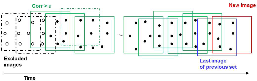
We have two classes of parameters, i.e., EOPs of each image and GPs corresponding to all the tie points. The parameters to be updated are selected separately from among previous parameters as a class. First, we select previous EOPs that are highly correlated with the EOPs of a new image by determining the correlation coefficient between EOPs. However, a problem arises because the correlation coefficient between the existing EOPs and the EOPs of a new image can be found only after adjusting for both existing parameters and new parameters. It is inefficient to adjust all previous parameters without excluding those that correlate poorly with new parameters. It is apparent that a new image is likely to be closest to the last image of the previous set, so we use the correlation coefficient between the EOPs of the previous images and the EOPs of the last image of the previous set instead of the EOPs of the new image. As shown in Figure 2, the last image (blue) instead of the new image (red) is employed to compute the correlation coefficient of the previous images. The EOPs of the image, whose correlation coefficients with the EOPs of the last image are less than a threshold, are excluded from the parameter vector to be updated. Each EOP set of two images has six parameters, X, Y, Z, ω, ϕ, and κ, referring to the position and attitude of the camera. Therefore, the correlation coefficients between the EOPs of the two images are presented as a 6 × 6 matrix. The maximum value among those 36 components in the correlation coefficient block is considered the correlation coefficient between the EOPs of the two images.
To facilitate the efficient implementation of this algorithm, there is no further examination of the correlation coefficient between the EOPs of the next images and the EOPs of the last image after an image highly correlated with the last image is detected from the beginning of the sequence. For example, if the correlation coefficient between the EOPs of the third image and those of the last image is more than the threshold for the first time, all of the EOPs from the third image to the last image should be updated, even though the correlation coefficient of the EOPs for the fifth and the last image is less than the threshold (Figure 2).
After the images associated with the EOPs included in the adjustment are selected, GPs appearing only in the images associated with EOPs excluded from the adjustment also have to be eliminated in the adjustment computation. Some GPs may appear only once in the images associated with the EOPs included in the adjustment. They should also be deleted from the adjustment computation because they can no longer be considered to be derived from tie points. As shown in Figure 2, white GPs do not appear or appear only once in the images associated with the EOPs included in the adjustment. Therefore, those white GPs are excluded from the parameter vector to be updated. Finally, the EOPs and GPs that are highly correlated with a new image are determined and the size of the parameter vector can be held nearly constant. The algorithm for keeping constant the parameter vector size is summarized below.

| Do if a new image is acquired |
| For n = 1: the number of previous images |
| Calculate the correlation coefficient between EOPs of a previous image and the new image. |
| If (the correlation coefficient < a threshold) |
| Exclude the EOPs of a previous image from the parameter vector. |
| Else |
| Count the number of images that appear per previous GP |
| If (the appearance number > 1) |
| Include the GP in the parameter vector |
3. Experiments with Simulated Data
Experiments were conducted with simulated data sets to evaluate our proposed AT algorithm. We implemented three types of aerial triangulation processes, the sequential AT with highly correlated images (Seq-R), the sequential AT with full images (Seq-F), and the simultaneous AT (Sim) using Matlab (ver. R2008b), and tested them in the computing environment described in Table 1. Each AT method was applied with simulated data and the results were analyzed in terms of accuracy and processing time.
3.1. Preparation for Experiments
Emergency monitoring will definitely benefit from real-time image georeferencing technologies. In an emergency situation, we need a feasible platform such as an unmanned aerial vehicle (UAV). One of the advantages of utilizing an UAV is that it can fly over dangerous regions without a human operator. In addition, it enables us to acquire sensory data with high spatial resolution since it can fly at relatively low altitude. Thus, we assumed a multi-sensor system based on a close-range UAV to simulate experimental data. We assumed that the system is equipped with a medium-format digital camera and a medium-grade GPS/INS. These sensors were carefully selected among the actual sensors available in current markets and their specifications were used for the simulation parameters. Under reasonable assumptions for flight and sensor parameters and a terrain model, we determined the attitude and position of the camera at the time of exposure of each image and the tie points in the adjacent images. The main simulation parameters are summarized in Table 2.
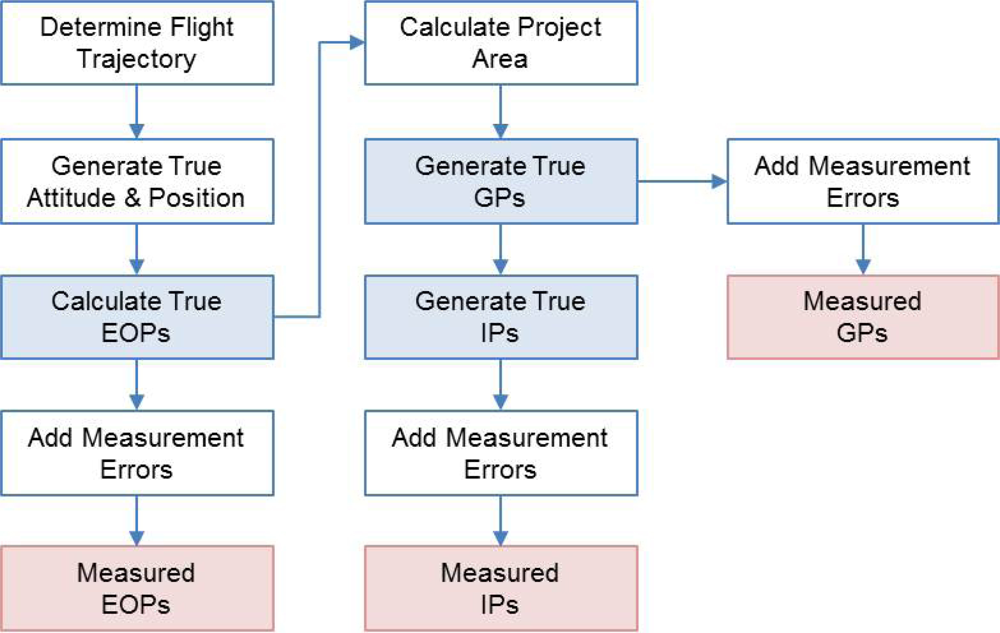
The simulation procedure is shown in detail in Figure 3. First, we determined a flight trajectory and acceleration and angular acceleration along the trajectory. We determined the true attitude and position by substituting the acceleration and the angular acceleration into the navigation equation. By sampling the attitude and position at the frame rate, true exterior orientation parameters (EOPs) were obtained. We simulated the measured EOP pos (position) and EOP att (attitude) by adding position and attitude measurement errors to the true EOPs, respectively. Then, we produced true ground point coordinates (GPs) within the project areas boundaries, which were determined according to the true EOPs and image coverage. The true image point coordinates (IPs) were generated through back-projection based on collinearity equations. Finally, we simulated the IPs by adding measurement errors, 1 pixel size, to the true IPs. We assigned the standard deviations of the position and attitude errors as 0.3 m and 0.1° by assuming a SBAS (Satellite Based Augmentation System) GPS/INS system.
There were a total of 5,812 simulated images points and 304 ground points, and an average of 14.4 conjugate points between adjacent images. The overlap ratio between two subsequent images was almost 94%. One ground point appeared in 20 images on average except at the fringes of the project area. The results of the simulation are summarized in Table 3. We implemented three types of AT processes and compared them quantitatively, denoted as Sim, Seq-F, and Seq-R. The first is the traditional simultaneous AT; the second is the sequential AT considering all the previous images; the third is the sequential AT considering only the images that are highly correlated with the newest image. In the third process, we exclude images for which the correlation with the last image in the previous set was less than a threshold. The threshold can be variably defined based on processing time requirements and the accuracy of AT results.
3.2. Accuracy Verification
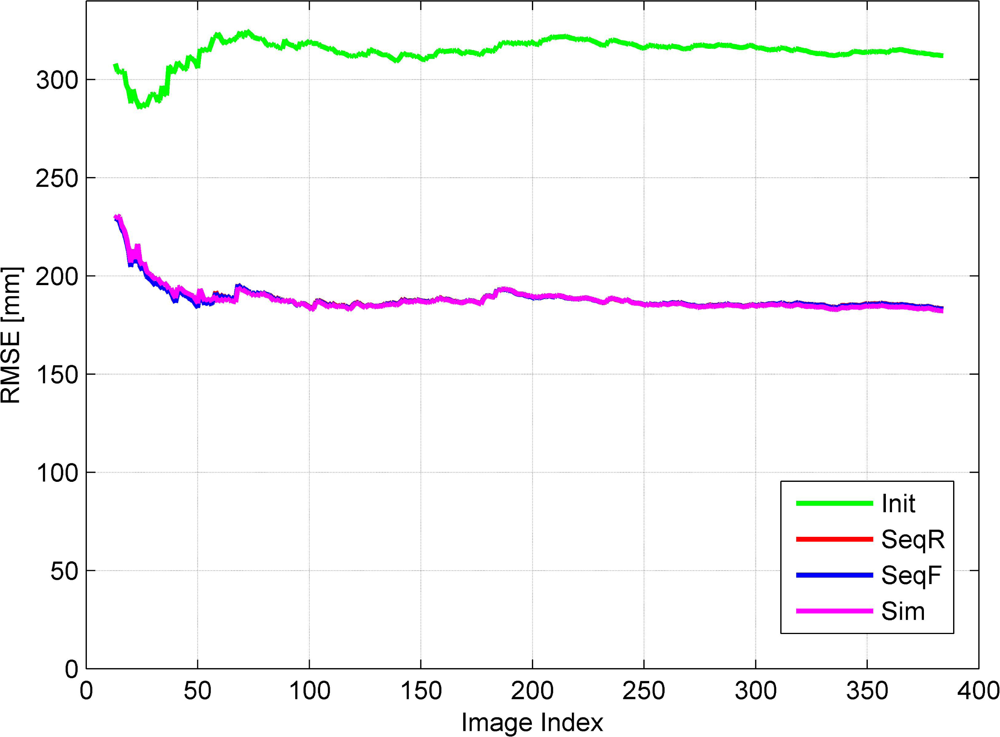
By applying the simulated data to the three different AT processes, we can estimate the EOPs and GPs whenever a new image is acquired. Since the input data are a simulated set, we know the true values for all the unknowns and compute the RMSE by comparing them with the estimated ones. Figures 4 and 5 show the RMSEs of the estimates for the position and attitude parameters among EOPs, respectively. The green lines represent the RMSE of the initial approximations, which indicate the accuracy of the direct measurements by the GPS/INS. The RMSE of the initial approximations, about 0.32 m and 0.1°, corresponds to the assumption about the GPS/INS quality parameter in Table 1, as expected.
The red, blue and pink lines represent the RMSE of the estimates from the sequential AT with only highly correlated images (Seq-R), the sequential AT with full images (Seq-F), and the simultaneous AT (Sim), respectively. The results from all types of AT are evidently better than the initial approximation the results from direct georeferencing. In addition, the results from each AT method are very similar. We see that the red, blue and pink lines almost coincide. The RMSEs of the estimated EOPs from each method are about 0.18 m and 0.05°. This is nearly a 50% improvement in accuracy compared with the results of direct georeferencing. Indirect georeferencing technologies based on aerial triangulation can compensate for position/attitude sensor performance such as in GPS/INS. Figure 6 shows the RMSE of the estimates for the GPs. The initial approximation for GPs can be computed using the tie points and the initial EOPs provided by GPS/INS. The RMSE of the initial approximation for GPs is about 1 m, which is quite reasonable considering the propagation of GPS/INS, IP and GP measurement errors to GP estimates. Through indirect georeferencing, such as Sim, Seq-F and Seq-R, the RMSE for GP is significantly reduced from about 1 m to 10 cm. All the parameters can be estimated through Seq-F or even Seq-R without large decreases in the RMSE, as compared with the RMSE of Sim.
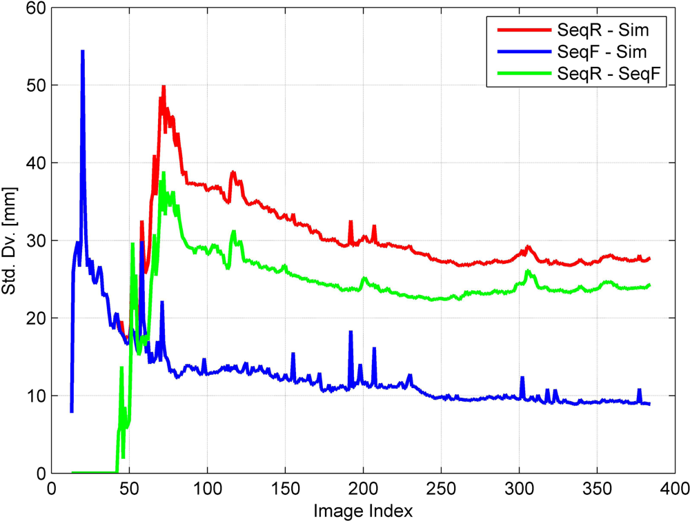
To compare the results from these methods, we compute the standard deviation of the differences between the ground point coordinates estimated using the three different methods, as shown in Figure 7. The blue line indicates the standard deviation of the difference between the results from Seq-F and Sim. The differences are relatively large for about 20 images in the beginning of the sequence. Thereafter, the differences decrease considerably and finally come within ± 1 cm. With the Seq-R results, the differences are limited to within ± 3 cm even though some previous images are excluded for faster computation. We can perform georeferencing of an image sequence using sequential AT with only highly correlated images and have accuracy of ± 3 cm compared with a post-processing method, simultaneous AT. In this experiment, the correlation coefficient threshold to exclude the less correlated images is set to 0.1.
3.3. Processing Time
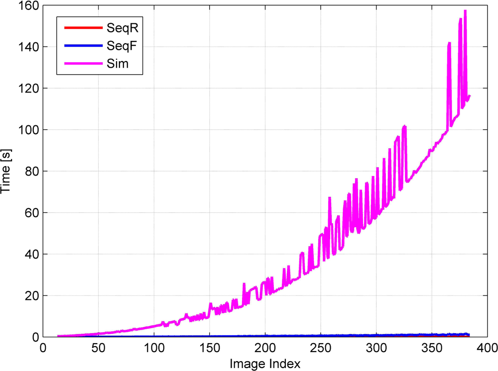
The goal of sequential AT is to determine the EOP of all the images in almost real time whenever a new image is acquired. Therefore, it is necessary to prove that sequential AT is more efficient than simultaneous AT in terms of processing time. Figure 8 shows the processing time of each method according to the number of images being acquired within an image sequence. The pink line denotes the processing time of the simultaneous AT. The blue line and red line represent the processing time of the sequential AT with full images and the sequential AT with only highly correlated images, respectively. From the comparison of the processing times, we found that the processing time of sequential AT is much shorter than that of simultaneous AT, as expected.
The processing time of simultaneous AT increases proportionally to the square of the number of images as shown in Figure 8. Many peaks appearing on the graph that indicate the processing time of simultaneous AT arise since the number of iterations is varied to solve the non-linear problem. Simultaneous AT requires significantly more computation time than sequential AT mainly because the dimension of the inverse normal matrix increases remarkably due to the increasing number of images. In spite of the reduced normal matrix scheme, we have to compute two kinds of inverse normal matrices (
and
) with dimensions that depend on the number of total images and GPs. The dimensions are (ne × 6) and (ngp × 3), where ne and ngp are the total number of images and GPs, respectively. As image acquisition progresses, it is obvious that the dimensions rapidly increase according to the increasing number of total parameters, EOPs and GPs. However, with our sequential methods, both Seq-F and Seq-R, inverse operations required at each stage, are only
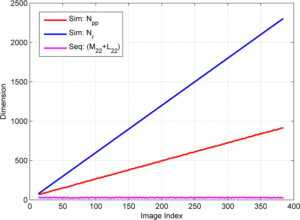
and (M22 + L22)−1 as indicated earlier. Their dimensions depend principally on the number of newly acquired observations and thus can be maintained as a small constant. The sizes of Nr and Npp increase almost linearly according to the number of images, while the size of (M22 + L22) is maintained almost constantly with slight changes, as shown in Figure 9. The increase in the sizes of Nr and Npp is not suitable for real-time georeferencing. Consequently, simultaneous AT cannot be employed for applications requiring real-time georeferencing even though it provides highly accurate results.
The processing time of sequential AT with full images also increases slightly with the number of images as shown in Figure 10, which is an enlargement of Figure 8. This is because the size of the parameter vector to be updated increases linearly with the number of images. The time to update the parameter thus increases linearly, although the inverse normal matrix can be computed within a constant time frame, regardless of the number of images. This linear increase makes real-time processing impossible when the image sequence is long and comprises a large number of images. The processing time at each stage must be limited to a constant to facilitate real-time processing.
Sequential AT with highly correlated images can be useful for real-time processing for a long image sequence. In such a sequence, it is obvious that some images in the beginning of the sequence must have almost no correlation with a new image. Hence, we choose not to update the parameters associated with the images in the beginning of the sequence. Here, the question is how many images in the beginning of the sequence can be safely excluded from the adjustment. Instead of setting a particular number of images to be excluded, we adaptively select the images that would have an almost negligible impact on the adjustment by determining their correlation with the new image. Such images with EOPs that have a low correlation coefficient with the EOPs of the new image can be reasonably excluded from the adjustment.
In the experiment, we exclude the images with correlation coefficients less than 0.1. With this threshold, the size of the parameter vector is maintained at about 400 (Figure 11). The processing time of Seq-R can be limited to 0.1 s (Figure 10). Since a new image is acquired every 0.5 s, the processing time is fully satisfactory for real-time image georeferencing. Furthermore, the speed requirement of a specific application can be fulfilled by selecting an appropriate threshold for the correlation coefficient.
4. Application to Real Data
4.1. Data Preparation
We acquired the real data using an airborne multi-sensory system composed of an UAV and sensors such as a digital camera, a laser scanner, and GPS/INS. The main specifications of the sensors are summarized in Table 4. The test site covers residential, agricultural and river areas in Chungju, Korea. The flight altitude and velocity are 200 m and 60 km/h, respectively. The flight trajectory is shown over the test site in Figure 12. The system during the data acquisition is presented in Figure 13.
We obtained 113 images with a GSD (Ground Sampling Distance) of 3 cm and performed automatic image matching using a commercial digital photogrammetric workstation to generate conjugate points, the input data for AT. A total of 1,488 conjugate points corresponding to 304 ground points are produced with an average of 13 conjugate points between adjacent images. The coverage of the images and the distribution of the ground points are shown in Figure 14. The green dots indicate the ground points and the red dots indicate the camera positions at the exposure times.
4.2. Results and Analysis
We applied our sequential AT algorithms to the real data and analyzed the results in terms of the accuracy and processing time. To verify the accuracy, we compared the estimates from our AT methods (Seq-R and Seq-F) with those from the conventional AT method (Sim). Since we do not know the true values for the unknowns in the experiments using real data, we used the Sim results as the reference data instead. The Sim results have been recognized as the most accurate, although Sim cannot be performed in real time.
The AT results are verified in terms of EOP positions, EOP attitudes, and GPs. The RMS values of the differences between three AT results are shown in Figures 15–17. Our algorithm operates the same as the Sim algorithm in the initial stage when a small number of images are acquired. The differences are thus presented after the 11th image. When the sequential combined stage starts from the 11th image, the RMS values increase dramatically and decreases gradually while new images are continuously acquired. When the final image is acquired, the RMS values of the differences between Seq-R and Sim estimates on EOP positions, EOP attitudes, and GPs reach about 0.7 mm, 0.0006° and 5 cm, respectively. It is important that the results from our algorithm are increasingly similar to those from Sim as the sequential stage progresses.
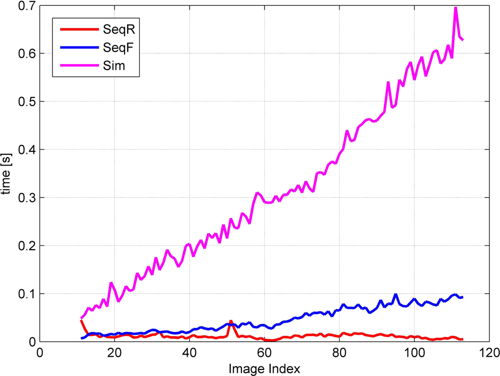
The processing times of each AT method according to the number of images being acquired are shown in Figure 18. As we expect, the processing time of Sim increases drastically according to the number of images, which makes it impossible to operate in real time. Only the Seq-R consumes a bounded time, less than 0.1 s, regardless of the number of images.
5. Conclusions
This research proposes a new sequential AT algorithm to perform real-time georeferencing of image sequences acquired by an airborne multi-sensor system. Although the traditional AT algorithm can produce very accurate results, it cannot be employed for real-time georeferencing due to its computation time, which dramatically increases with the number of images. The proposed sequential AT algorithm can produce accurate results comparable to those from the simultaneous AT with a computation time maintained within a constant time frame. This algorithm can be controlled such that it has a computation time shorter than the image acquisition time, which supports real-time georeferencing. Rapid computation is possible since only the minimum computation at the current stage is performed, using the computational results from the previous stage whenever a new image is added. Moreover, the exclusion of an image based on the correlation between the existing and new parameters in the algorithm can minimize the processing time.
The accuracy and processing speed were verified by applying this algorithm to a simulated data set. The experimental results show that the georeferencing of an image sequence is possible in less than 0.1 s whenever a new image is acquired every 0.5 s. The accuracy of the sequential AT results is comparable to that from the simultaneous AT results, where the differences between both results are very small, within ±3 cm in terms of the ground point coordinates. In addition, the proposed algorithm was applied to a real data set acquired by an airborne multi-sensory system and the results confirm that it works efficiently with the real data as well as the simulated data.
Consequently, it is expected that our sequential AT algorithm can be effectively employed for various applications requiring real-time image georeferencing such as disaster monitoring and image-based navigation. In the near future, this sequential AT algorithm will be integrated with a real-time image matching algorithm for real-time image georeferencing. Finally, this approach will be applied to a variety of real data sets and also verified with respect to accuracy and processing speed.
References
- Choi, K.; Lee, I.; Hong, J.; Oh, T.; Shin, S. Developing an UAV based rapid mapping system for emergency response. Proc. SPIE 2009. [Google Scholar] [CrossRef]
- Choi, K.; Lee, I.; Shin, S.W.; Ahn, K. A project overview for the development of a light and flexible rapid mapping system for emergency response. Int. Arch. Photogramm. Remote Sens. Spat. Inf. Sci 2008, 37, 915–920. [Google Scholar]
- Choi, K.; Lee, J.; Lee, I. A UAV Multi-sensor Rapid Mapping System for Disaster Management. Proceedings of Geoinformation for Disaster Management (Gi4DM), Antalya, Turkey, 3–8 May 2011.
- Choi, K.; Lee, I. A UAV-based close-range rapid aerial monitoring system for emergency responses. Int. Arch. Photogramm. Remote Sens. Spat. Inf. Sci 2011, 38, 247–252. [Google Scholar]
- Rau, J.; Habib, A.; Kersting, A.; Chiang, K.; Bang, K.; Tseng, Y.; Li, Y. Direct sensor orientation of a land-based mobile mapping system. Sensors 2011, 11, 7243–7261. [Google Scholar]
- McGlone, C. Manual of Photogrammetry, 5th ed.; American Society of Photogrammetry and Remote Sensing: Bethesda, MD, USA, 2004. [Google Scholar]
- Mikhail, E.; Helmering, R. Recursive methods in photogrammetric data reduction. Photogramm. Eng 1973, 39, 983–989. [Google Scholar]
- Gruen, A. An optimum algorithm for on-line triangulation. Int. Arch. Photogramm. Remote Sens. Spat. Inf. Sci 1982, 24, 1–22. [Google Scholar]
- Blais, J. Linear least-squares computations using Givens transformation. Can. Surv 1983, 37, 225–233. [Google Scholar]
- Matthies, L.; Szeliski, R.; Kanade, T. Kalman filter-based algorithms for estimating depth from image sequences. Int. J. Comput. Vis 1989, 3, 209–238. [Google Scholar]
- Gruen, A. Algorithmic aspects in on-line triangulation. Photogramm. Eng. Remote Sensing 1985, 51, 419–436. [Google Scholar]
- Runge, A. The Use of Givens Transformation in On-Line Triangulation. Proceedings of ISPRS Intercommission Conference on Fast Processing of Photogrammetric Data, Interlaken, Switzerland, 2–4 June 1987; pp. 179–192.
- Holm, K. Test of algorithms for sequential adjustment in on-line phototriangulation. Photogrammetria 1989, 43, 143–156. [Google Scholar]
- Gruen, A.; Kersten, T. Sequential estimation in robot vision. Photogramm. Eng. Remote Sensing 1995, 61, 75–82. [Google Scholar]
- Kersten, T.; Baltsavias, E. Sequential estimation of sensor orientation for stereo images sequences. Int. Arch. Photogramm. Remote Sens. Spat. Inf. Sci 1994, 30, 206–213. [Google Scholar]
- Edmundson, K.; Fraser, C. A practical evaluation of sequential estimation for vision metrology. ISPRS J. Photogramm 1998, 53, 272–285. [Google Scholar]
- Dogan, S.; Temiz, M.; Kulur, S. Real time speed estimation of moving vehicles from side view images from an uncalibrated video camera. Sensors 2010, 10, 4805–4824. [Google Scholar]
Figure 1.
Real-time image georeferencing.
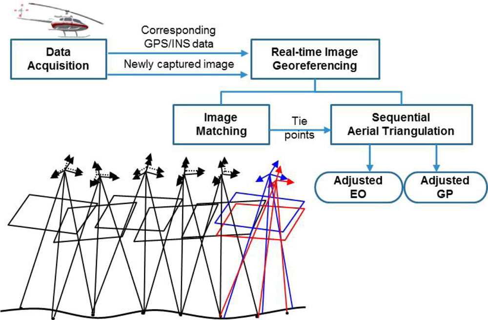
Figure 2.
Exclusion process of the previous parameters.

Figure 3.
Simulation procedures.

Figure 4.
RMSE of estimated EOP (position).

Figure 5.
RMSE of estimated EOP (attitude).
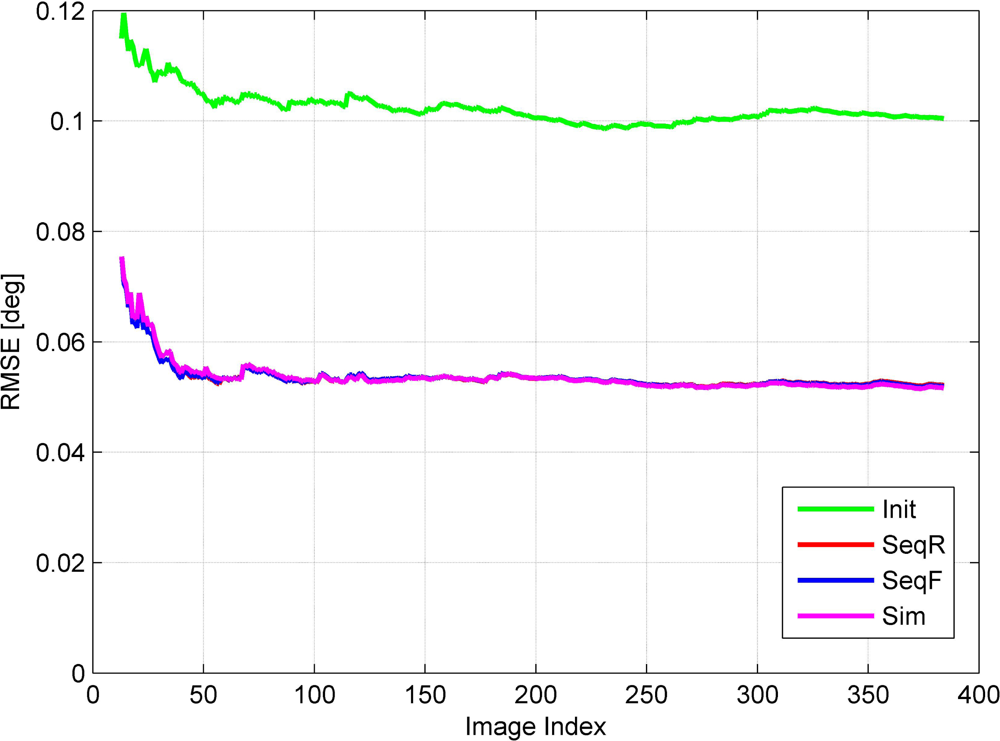
Figure 6.
RMSE of estimated ground point coordinates.
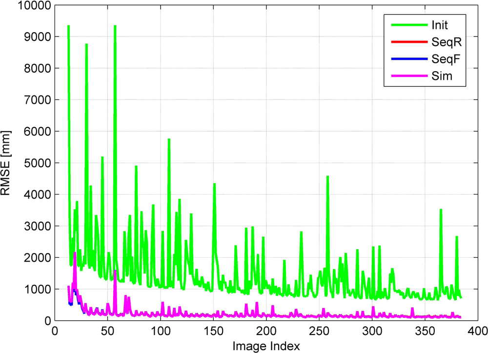
Figure 7.
Standard deviation of estimated ground point coordinates.

Figure 8.
Processing time of the three AT methods.

Figure 9.
Dimension of the inverse matrices to be computed.

Figure 10.
Processing time of the three AT methods (zoomed in).
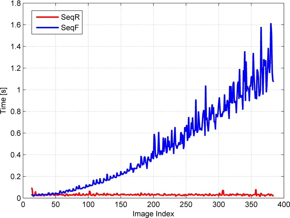
Figure 11.
Size of parameter vectors.

Figure 12.
Test site and flight trajectory.
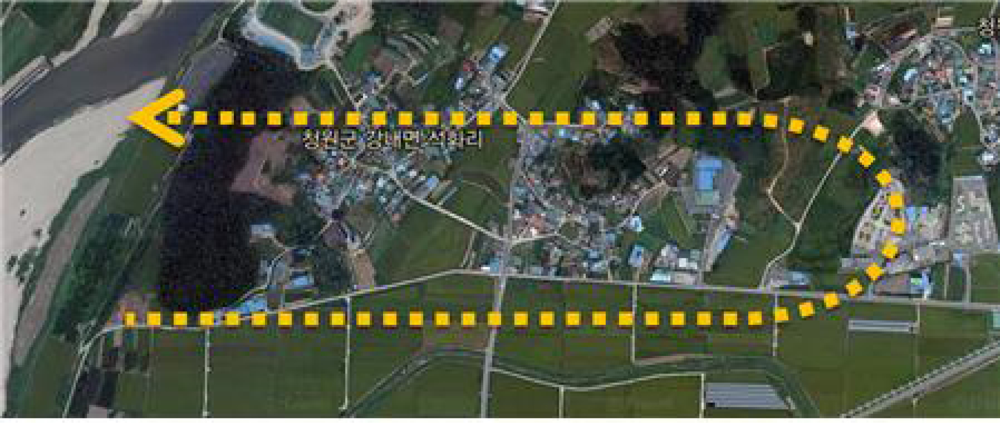
Figure 13.
Airborne multi-sensory system during data acquisition over the test site.
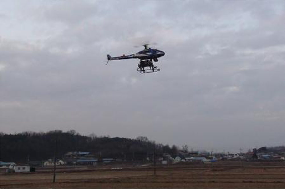
Figure 14.
Image coverage and ground points.
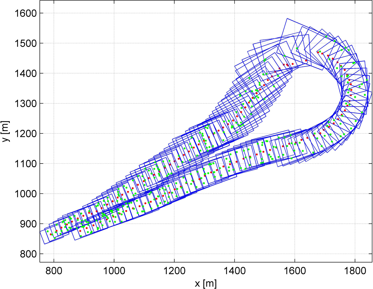
Figure 15.
RMS values of EOP differences (position).

Figure 16.
RMS values of EOP differences (attitude).
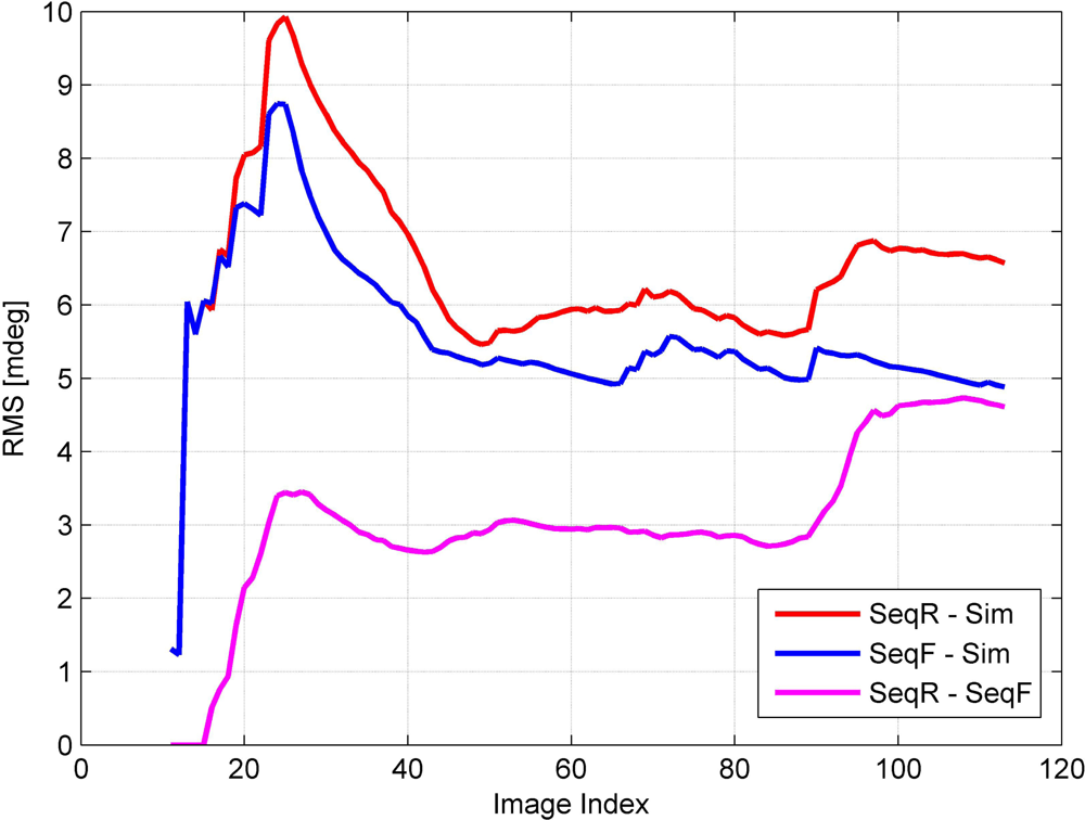
Figure 17.
RMS values of GP differences.
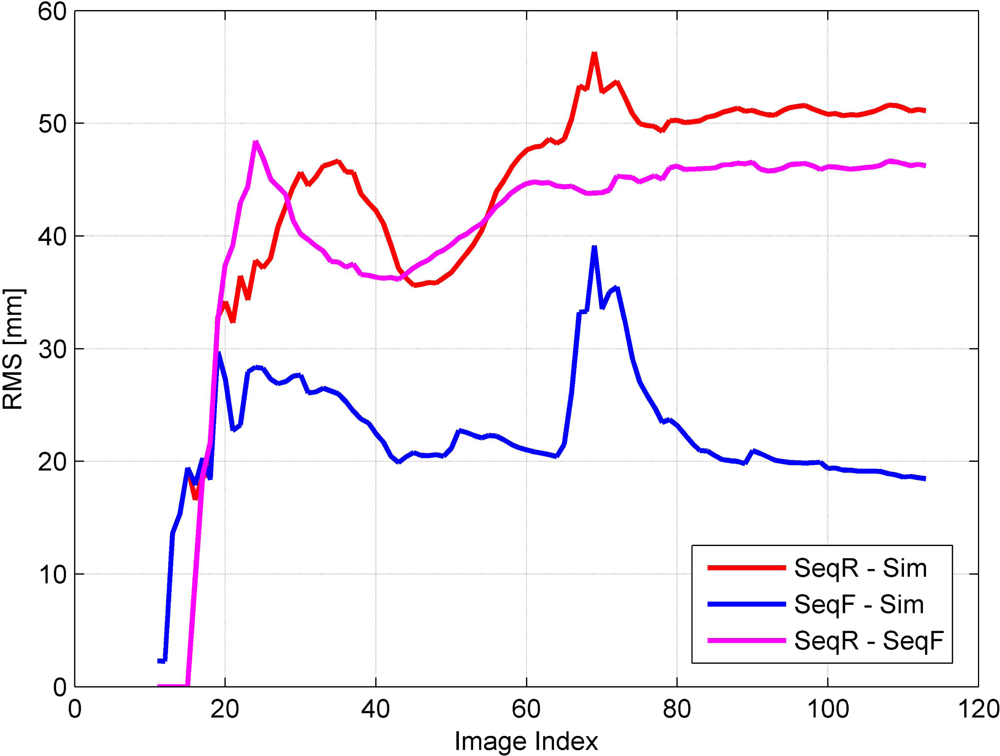
Figure 18.
Processing time of each AT method.
| Environment | Specifications |
|---|---|
| Operating System | Microsoft Window XP SP3 |
| CPU | Intel(R) Core(TM)2 Duo CPU |
| E7500 @ 2.93 GHz, 2.93 GHz | |
| RAM | 3.00 GB |
| Category | Parameter | Value | Unit |
|---|---|---|---|
| Flight configuration | height | 200 | m |
| speed | 10 | m/s | |
| no. strips | 1 | ||
| length of a strip | 2,000 | m | |
| Camera | focal length | 17 | mm |
| pixel size | 3.45 × 3.45 | μm | |
| detector dimensions | 2,456 × 2,058 | pixels | |
| frame rate | 2 | images/s | |
| GPS/INS | position error | 0.3 | m |
| attitude error | 0.1 | degree |
| Parameter | Value |
|---|---|
| Images per strip | 384 |
| Ground points | 304 |
| Image points | 5,812 |
| Image points per ground point | 20 |
| Tie points between adjacent images | 14 |
| Ground Sampling Distance (GSD) | 3 cm |
| Sensors | Specifications |
|---|---|
| Camera | medium format |
| effective pixels : 4,872 × 3,248 | |
| focal length : 50 mm | |
| frame rate : 1 fps | |
| GPS/INS | tactical grade |
| position accuracy : 0.3 m | |
| attitude accuracy : 0.1° | |
| data rate : 20 Hz | |
Share and Cite
MDPI and ACS Style
Choi, K.; Lee, I. A Sequential Aerial Triangulation Algorithm for Real-time Georeferencing of Image Sequences Acquired by an Airborne Multi-Sensor System. Remote Sens. 2013, 5, 57-82. https://doi.org/10.3390/rs5010057
AMA Style
Choi K, Lee I. A Sequential Aerial Triangulation Algorithm for Real-time Georeferencing of Image Sequences Acquired by an Airborne Multi-Sensor System. Remote Sensing. 2013; 5(1):57-82. https://doi.org/10.3390/rs5010057
Chicago/Turabian StyleChoi, Kyoungah, and Impyeong Lee. 2013. "A Sequential Aerial Triangulation Algorithm for Real-time Georeferencing of Image Sequences Acquired by an Airborne Multi-Sensor System" Remote Sensing 5, no. 1: 57-82. https://doi.org/10.3390/rs5010057