Analysis and Inter-Calibration of Wet Path Delay Datasets to Compute the Wet Tropospheric Correction for CryoSat-2 over Ocean

Abstract

Unlike most altimetric missions, CryoSat-2 is not equipped with an onboard microwave radiometer (MWR) to provide wet tropospheric correction (WTC) to radar altimeter measurements, thus, relying on a model-based one provided by the European Center for Medium-range Weather Forecasts (ECMWF). In the ambit of ESA funded project CP4O, an improved WTC for CryoSat-2 data over ocean is under development, based on a data combination algorithm (DComb) through objective analysis of WTC values derived from all existing global-scale data types. The scope of this study is the analysis and inter-calibration of the large dataset of total column water vapor (TCWV) products from scanning MWR aboard Remote Sensing (RS) missions for use in the WTC computation for CryoSat-2. The main issues regarding the computation of the WTC from all TCWV products are discussed. The analysis of the orbital parameters of CryoSat-2 and all other considered RS missions, their sensor characteristics and inter-calibration is presented, providing an insight into the expected impact of these datasets on the WTC estimation. The most suitable approach for calculating the WTC from TCWV is investigated. For this type of application, after calibration with respect to an appropriate reference, two approaches were found to give very similar results, with root mean square differences of 2 mm.

1. Introduction

With an absolute value up to 50 cm and highly variable in space and time, the path delay due to the presence of water vapor in the atmosphere, or wet tropospheric correction (WTC), is still one of the major error sources in satellite radar altimetry. Due to its high variability, the most accurate way to model this effect over open ocean is through the measurements of microwave radiometers (MWR) on board the altimetric missions.

CryoSat-2 (CS-2), primarily dedicated to measuring and monitoring the changing thickness of ice in polar regions, does not carry an onboard MWR, being the wet tropospheric correction currently applied to the radar altimeter data, a model-based one, provided by the European Center for Medium-Range Weather Forecasts (ECMWF). The loss of Envisat in April 2012 increased the use of CS-2 data for applications beyond the primary objectives of the mission, including studies over oceans. The more stringent accuracy requirements imposed by global-scale ocean and coastal studies, however, are driving a need to develop an improved correction for CS-2, particularly important for these applications.

In the scope of the European Space Agency (ESA) funded project “CryoSat Plus for Oceans (CP4O)” (e.g., [1]), a data combination (DComb) algorithm is being developed for the computation of a more accurate WTC, when compared to the one provided by ECMWF. The DComb algorithm, based on the approaches followed by [2–4], estimates the WTC using objective analysis of several available data sources: Scanning MWR on board remote sensing (RS) satellites, Global Navigation Satellite Systems (GNSS), and the ECMWF ReAnalysis (ERA) Interim model. The purpose of the present study is the analysis and inter-calibration of some of the datasets used in the computation of the wet path delay of altimeter measurements over ocean, including open ocean, polar regions, and coastal zones, for their use in the DComb algorithm. In this context, the dataset of total column water vapor (TCWV) images acquired by the various scanning MWR on board RS missions is of particular relevance due to data amount and coverage (both in space and time) and the variety of instruments acquiring such data, which will thus require proper inter-calibration. The analysis and inter-calibration of the WTC derived from these TCWV images is the main focus of this study.

In Section 2, the WTC estimation from microwave radiometers is addressed and the main issues regarding the WTC estimation from TCWV datasets are discussed.

A detailed analysis and inter-calibration of the water vapor products of scanning MWR of various sensors on board different RS missions and the main issues concerning their use and impact in the improvement of the WTC for CS-2 are analyzed in Section 3. Discussion and main conclusions are presented in Section 4.

2. WTC Estimation from Microwave Radiometers

2.1. Introduction

The correction for the path-delay of the altimeter signal due to the presence of water vapor in the atmosphere is one of the most difficult altimeter corrections to model. The magnitude of this correction is much smaller than the corresponding dry component, which is of the order of 2.3 m but can be precisely modeled (accuracy better than 1 cm, [3]) from meteorological models which assimilate atmospheric temperature and pressure measurements. The wet component is much more difficult to estimate because of the high variability of humidity and the complexity of the water cycle at all spatial and time scales.

Mean values of WTC show a near-zonal dependency, with absolute values ranging from less than 5 cm at high latitudes to ∼35 cm near the equator and the tropics (Figure 1). The standard deviation ranges from 1–5 cm near the poles to 10–15 cm in the tropics (Figure 2).

In spite of the continuous progress in the modeling of this effect by means of numerical weather models (NWM) (e.g., [5,6]), accuracy of present NWM-derived WTC is still not good enough for most altimetry applications such as sea level variation. Indeed, an accurate enough modeling of this effect can only be achieved through actual measurements of the atmospheric water vapor content at the time and location of the altimetric measurements. For this purpose, dedicated microwave radiometers have been incorporated in the most recent altimetric missions. For simplicity, these instruments will be hereafter designated by RA-MWR, standing for near nadir-looking, single measurement MWR on board radar altimeter missions. Two main types of RA-MWR have been used: 2-band and 3-band radiometers. Examples of the first are those flown on European Remote-sensing Satellite (ERS), Geosat Follow-On (GFO), Envisat, SARAL/Altika, and the upcoming Sentinel-3; TOPEX/Poseidon (T/P), and Jason-1 (J1) and Jason-2 (J2) possess 3-band radiometers. All of them have one band in the water vapor absorption line between 21 and 23.8 GHz plus one or two in “atmospheric window” channels. The 2-band radiometers have the second band in the 34–37 GHz window, sensitive to surface emissivity and also sensitive to cloud liquid water; the 3-band radiometers have a third channel near the 18–18.7 GHz band, also sensitive to surface emissivity and with particularly low sensitivity to clouds, improving the retrieval of the atmospheric correction [7,8]. In the 2-band microwave radiometers, which do not include the low frequency channel, the surface roughness is taken into account through the altimeter backscattering coefficient. The spatial resolution of these instruments is of the order of 20–45 km [9], except for AltiKa, which is about 10 km [10,11].

In addition to the dedicated MWR aboard altimetric missions, scanning imaging instruments, also retrieving water vapor data from measurements in several bands of the microwave spectrum, have been flown in various RS missions. In addition, for simplicity, these instruments will hereafter be designated by SI-MWR, standing for scanning imaging MWR, not to be confused with the RA-MWR single-measurement systems. The main difference between RA-MWR and SI-MWR is that, at each epoch, the first can only make a single measurement in the nadir direction while the second performs a scan of the sea surface over the instrument swath. While the final product of the first is an along track profile, the second is an along-track image. The details of the instruments and water vapor products available for the various SI-MWR are presented in Section 3.

2.2. From TCWV to WTC

The total column water vapor, also referred as precipitable water, PW, or integrated water vapor, (IWV) is the total water vapor contained in an air column from the Earth’s surface to the top of the atmosphere and is usually expressed in kg/m² or millimeters (mm), as the length of an equivalent column of liquid water.

The TCWV (abbreviated to WV in the following equations) in kg/m² is given by

$$\mathit{WV}=\underset{0}{\overset{H}{\int }}{\rho }_w\mathit{dz}$$

(1)

where ρ_w is the water vapor density in kilograms per cubic meter, z is the altitude (in m), and H is the altitude above which the water vapor density is considered to be negligible. Dividing the above equation by the density of liquid water ρ (ρ = 10³ kg/m³) the equivalent quantity in millimeters is obtained [12].

The path delay due to the water vapor in the atmosphere, the WTC, can be estimated from TCWV and atmospheric temperature T by (e.g., [13]):

$$\mathit{WTC}=1.763\underset{0}{\overset{H}{\int }}\frac{{\rho }_w}{T}\mathit{dz}$$

(2)

where WTC is in meters and T is the temperature in kelvin.

For practical computations it is most appropriate to replace the vertical integration expressed in Equation (2) by expressions which make use of single level quantities as provided by NWM or measured quantities as provided by most measurement systems.

The relation between WTC and TCWV is a function of various physical constants and of the weighted mean temperature T_m of the atmosphere. According to [12,14], the WTC can be estimated from TCWV and T_m using the following expression:

$$\mathit{WTC}=-\left(0.101995+\frac{1725.55}{T_m}\right)\frac{\mathit{WV}}{1000}$$

(3)

where T_m is the mean temperature of the troposphere, which may be in turn modeled from the surface temperature (T₀) according to, e.g., [15,16]:

$$T_m=50.40+0.789\hspace{0.17em}{T}_0$$

(4)

In Equations (3) and (4), T₀ and T_m are in kelvin, WV in millimeters and the WTC results in meters. A similar expression to Equation (4) was derived by [12]. According to [15,16], Equation (4) was determined using a global set of radiosondes covering a latitude range of 62°S to 83°N, while [12] used a set of sites in the United States, with a latitude range of 27°N to 65°N. In addition, the RMS of fit of the linear regressions of the derived models using radiosonde data is of 4.7 K [12] and 3.1 K [16], respectively. This should lead to errors in TCWV less than 2% [12,14,17]. Moreover, the T_m vs. T₀ relationship can be site-dependent and may vary seasonally and diurnally [17,18].

Alternatively, the dependence of the WTC on the atmospheric temperature can be implicitly accounted for by establishing a direct relationship between WTC and TCWV (e.g., [4,13,19]), since the ratio between WTC and TCWV can be described by a decreasing function of water vapor content, which partly expresses the WTC temperature dependence. For example, in [4] the following relationship was deduced from temperature and humidity profiles from ECMWF model fields:

$$\frac{\mathit{WTC}}{\mathit{WV}}=-(a_0+a_1\mathit{WV}+a_1{\mathit{WV}}^2+a_{3}W{V}^3)$$

(5)

with a₀ = 6.8544, a₁ = −0.4377, a₂ = 0.0714, a₃ = −0.0038. In Equation (5)WTC and WV are in centimeters. Keeping WV in cm, the corresponding WTC values in meters are obtained as:

$$\mathit{WTC}=-(a_0+a_1\mathit{WV}+a_2{\mathit{WV}}^2+a_3{\mathit{WV}}^3)\hspace{0.17em}\mathit{WV}{.10}^{-2}$$

(6)

In [19], a similar expression is provided which gives WTC values about 1% larger than those given by Equation (5) [4].

For less accurate studies, the WTC can be considered approximately proportional to WV by

$$\mathit{WTC}(\text{m})=-0.0067\hspace{0.17em}\mathit{WV}(\text{mm})$$

(7)

In this study, both Equation (3) and Equation (6) are considered in order to identify the most suitable for use in the WTC retrieval from SI-MWR water vapor products. All expressions above provide the WTC in meters according to the convention adopted in altimeter Geophysical Data Records (GDR): the correction that should be added to the raw altimeter measurement to get the corrected one.

2.3. WTC from ERA Interim

At present, various global NWM exist for this type of application, such as ECMWF and the National Centre for Environment Prediction (NCEP). In this work ECMWF was adopted. Various versions of the ECMWF model are available, for example, the operational model at 0.125° × 0.125° or 0.25° × 0.25° spacing and six-hour intervals and the ERA Interim model at 0.75° × 0.75° spacing and also at six-hour intervals. Both model versions provide global grids of TCWV and surface temperature (two-meter Temperature, 2T). From these single-level fields, at each grid node, the wet tropospheric correction for altimeter measurements can be computed from TCWV and 2T using Equations (3) and (4).

Aiming to identify the most suitable version of the ECMWF model for use in the DComb algorithm, the WTC computed both from ERA Interim and ECMWF operational models, for the period of the three reference altimetric missions (T/P, J1, and J2) were compared, using the model values present in the Radar Altimeter Database System (RADS). In RADS, the WTC is estimated from ERA Interim 0.75°× 0.75° grids using the Bevis approach (Equations (3) and (4)); for the ECMWF operational model the WTC values are those present on the GDR of each mission. Results are shown in Figure 3, in which the statistical parameters (mean and standard deviation of the differences) for each mission cycle are plotted.

It can be observed that, since 1992, the operational model suffered various updates which originate discontinuities in the derived WTC. The mean differences between the two models reveal large discontinuities in the 90s (Figure 3a).

Figure 3b shows that the standard deviation of the differences between the two models decreases from about 3 cm in the early 90s to about 1 cm since 2004. Comparisons (not shown here) between each model and the WTC derived from the measurements of the RA-MWR of each altimetric mission show that, after 2004, both models agree with the MWR-derived WTC within 1.1–1.2 cm (1 standard deviation).

Comparisons with GNSS data presented in [3] show that for the latest years and in spite of its lower spatial resolution, the difference between GNSS-derived zenith total delays (ZTD) and those derived from ERA Interim and ECMWF operational model are very similar, with standard deviations of the order of 1.2 cm. The fact that, in spite of their different spatial resolution, both models give similar results, may be due to their poor temporal resolutions of six hours. In addition, the same authors also report the increase in the differences between GNSS and ECMWF operational derived ZTD as we go back in time, in agreement with Figure 3.

In summary, results show that ECMWF operational model is not suitable for use in altimetric studies over the years prior to 2004, if centimeter level accuracy is required. Since about 2004, the accuracy of ERA Interim model is similar to present ECMWF operational model and has the advantage of being homogeneous through time [6]. Consequently, in spite of its lower spatial resolution, ERA Interim has been identified as the most appropriate model for use in the DComb algorithm and throughout this study. It should also be emphasized that, although the first goal of the DComb type of WTC is CryoSat-2, it is aimed to apply the same methodology to any type of altimetric mission, including the oldest ones such as Geosat, which also does not possess an onboard radiometer). Therefore, the choice of ERA Interim warrants the same model accuracy for all missions.

2.4. WTC from SI-MWR Water Vapor Products

As mentioned above, scanning microwave imaging radiometers on board remote sensing satellites (SI-MWR) make measurements in various water vapor absorption bands of the microwave spectrum. The algorithm for retrieving the TCWV over the ocean using as input data from SI-MWR observations is usually based on a model using the brightness temperatures from channels operating at frequencies ∼19, ∼22, and 37 GHz; however, when using data from sensors such as AMSU-A, only observations from two channels are used (see

Table 1. Main characteristics of the sensors with scanning MWR images of TCWV available for this study. The scale factor of product is the value required to multiply the original product value to get the TCWV in mm. All products are swath except the last two, which are grid products.

Sensor	Pixel Size (km)	Swath Width (km)	Number of (Lines, Pixels)	Name of Product	Scale Factor of Product	Channels Used to Retrieve TCWV (GHz)
AMSR-E	9 km	1,625	(variable, 243)	Med_res_vapor	0.01	18.7/23.8/36.5
AMSU-A	50 km ***	2,200	(variable, 30)	TPW	0.1	23.8/31.4
TMI	10 km	878	(variable,104)	Columnar_water_vapor	0.01	19.35/21.3/37.0
SSM/I *	25 km	1,420	(variable,64)	TPW	0.1	19.35/22.235/37.0
SSM/I, SSM/IS **	0.25°	1,790–1,850	(720, 1440)	VAPOR	0.3	19.35/22.235/37.0
WindSat	0.25°	1,400	(720, 1440)	VAPOR	0.3	18.7/23.8/37.0

Note:

^*Swath product from NOAA CLASS database;

^**Grid product from Remote Sensing Systems (RSS);

^***Value provided is the central pixel size (maximum pixel size is 130 km).

and Section 3.1) [20–24].

As shown above, the WTC can then be derived from TCWV and atmospheric temperature using Equations (3) and (4), where the dependence on temperature can be accounted for from a NWM such as ERA Interim, or from a direct relationship such as that expressed by Equation (6). In this study both expressions will be used and their impact in the WTC estimation will be assessed.

3. MWR Imaging Sensors

3.1. Data Description

For use in the WTC estimation for CryoSat-2, a database of water vapor images was set up, encompassing all scanning MWR on board RS satellites whose data are available for the period of the CS-2 mission (starting in April 2010). The different sensors considered are (see Tables 1 and

Table 2. Main orbital characteristics (compared with those of CryoSat-2) of the satellites with scanning MWR images of TCWV available for this study. Grey-shaded rows refer to gridded products and the remaining to swath products. LTAN is the Local Time of the Ascending Node.

Satellite	Sensor	Height (km)	Inclination (°)	Period (min)	Sun-synch. Orbit	LTAN Jan 2011 (hh:mm)	LTAN Jan 2012 (hh:mm)	Data Availability for Cryosat-2
CryoSat-2	-	717	92.0	93.2	No	N/A	N/A	since April 2010
AQUA	AMSR-E	705	98.0	99.0	Yes	13:36	-	until Oct 2011
NOAA-19	AMSU-A	870	98.7	102.1	Yes	13:32	13:32	until present
NOAA-18	AMSU-A	854	98.7	102.1	Yes	14:07	14:30	until present
DMSP-F15	SSM/I	850	98.8	102.0	Yes	16:44	16:05	*
NOAA-15	AMSU-A	807	98.5	101.1	Yes	16:35	16:35	until present
Coriolis	WindSat	830	98.8	101.6	Yes	17:54	17:54	**
DMSP-F17	SSM/IS	850	98.8	102.0	Yes	17:30	18:06	until present
DMSP-F16	SSM/IS	845	98.9	101.8	Yes	19:12	18:30	until present
NOAA-17	AMSU-A	810	98.7	101.2	Yes	20:20	19:40	until present
NOAA-16	AMSU-A	849	99.0	102.1	Yes	19:16	20:00	until present
MetOp-A	AMSU-A	817	98.7	101.4	Yes	21:26	21:27	until present
TRMM	TMI	402	35.0	93.0	No	N/A	N/A	until present

^*CLASS products are available until present; RSS products, corrected for RADCAL beacon interference, are only available until end of 2011;

^**WindSat Version 7 of RSS products are only available until the end of 2011; after that date near real time (NRT) products are available.

):

(1)

The Advanced Microwave Sounding Unit A (AMSU-A) on board the National Oceanic and Atmospheric Administration (NOAA) satellite series (NOAA-15, -16, -17, -18, -19) and on board the European Organization for the Exploitation of Meteorological Satellites (EUMETSAT) MetOp-A satellite;

(2)

The Advanced Microwave Scanning Radiometer-Earth Observing System (AMSR-E) on board the National Aeronautics Space Administration (NASA) Aqua satellite;

(3)

The Tropical Rain Measuring Mission (TRMM) Microwave Imager (TMI) on board the joint NASA and Japan Aerospace Exploration Agency TRMM satellite;

(4)

The Special Sensor Microwave Imager (SSM/I) and Special Sensor Microwave Imager/Sounder (SSM/IS) on board the Defense Meteorological Satellite Program (DMSP) satellite series (F15, F16, F17, and F18);

(5)

The WindSat Polarimetric Radiometer developed by the Naval Research Laboratory (NRL) aboard Coriolis, a satellite of the US Department of Defense.

All data are available online and can be accessed as summarized below:

(1)

AMSU-A Level-2 swath products are made available by NOAA through its Comprehensive Large Array-Data Stewardship System (CLASS): http://www.class.ngdc.noaa.gov. The Microwave Surface and Precipitation Products System (MSPPS) Orbital Global Data products (MSPPS_ORB) have been used. In addition, CLASS also provides similar products for SSM/I (F15), although it was found that these products are not suitable for use in the WTC computation (see Section 3.3).

(2)

For the AMSR-E, the Level-2B ocean swath (AE_Ocean) dataset was downloaded from the National Snow and Ice Data Center (ftp://n4ftl01u.ecs.nasa.gov/SAN/AMSA/AE_Ocean.002/).

(3)

For TMI, the Level-2 product swath dataset was acquired from the Global Hydrology Resource Center (ftp://ghrc.nsstc.nasa.gov/pub/data/tmi-op/).

(4)

SSM/I and SSM/IS data are available through Remote Sensing Systems (RSS) ( http://www.ssmi.com/ssmi/ssmi_browse.html), which provide ocean data products for the DSMP satellites from F08 to F18. According to information in February 2013, products for F18 were not yet available. According to RSS information, after August 2006, F15 products are affected by RADCAL beacon interference. The released F15 Version 7 products from RSS have been corrected for this effect. Due to the required calibration and correction, F15 Version 7 products are provided with some delay; thus, for this study only data until the end of 2011 were available. In spite of the fact that RSS recommends that, after August 2006, F15 products should not be used for climate studies, it will be shown in Section 3.3 that the corrected (Version 7) RSS F15 products seem to be adequate for use in the WTC computations.

(5)

WindSat data are available through RSS (ftp://ftp.remss.com/windsat) also in the form of grid binary files; as for DMSP-F15 (see point 4 above) WindSat Version 7 products are being generated with some delay, and for the present study they were only available until the end of 2011—for the remaining period the near real time products are available. RSS also provides similar gridded products for AMSR-E.

Two types of water vapor products containing the TCWV field have been used: (1) Level-2 swath products, whenever available, from all data providers except RSS; (2) Level-2 gridded products, otherwise (from RSS). Swath products are available in HDF-EOS2 format, while gridded products are available in binary format. The existing products and their main characteristics are summarized in Tables 1 and 2 (status as in February 2013). Figures 4 and 5 show examples of the swath and gridded products, respectively.

3.2. Orbit Configuration

In this section we present an analysis of the characteristics of the orbits of the satellites providing the SI-MWR images and compare various orbital parameters with those of CryoSat-2, in view to understand the type of coverage that can be expected for CS-2 from these images.

When examining Table 2, the first remark is that, except for TMI, all MWR scanning sensors are on board satellites with sun-synchronous orbits with an inclination (98°–99°) close to that of CS-2 (92°). This means that the local time of ascending node (LTAN) of each satellite remains constant all over the year. On the contrary, since CS-2 orbit is not sun-synchronous, and with a very long repetition cycle (369 days), every day the satellite will have a pass over a different location and the corresponding LTAN will change accordingly. This means that the set of RS satellites that provide good space-time coverage for CS-2 at a given epoch, or, say, are in phase with CS-2, a few months later will be out of phase, with a large time difference between the acquisition time of the corresponding images and the CS-2 passage.

According to Table 1, leaving out the AQUA satellite, since AMSR-E stopped working on 4 October 2011, there are 10 RS missions in near polar sun-synchronous orbits providing water vapor products: NOAA-15, -16, -17, -18, -19, MetOp-A, DMSP-F15 (with some restrictions), -F16, -F17, and Coriolis. In summary, since October 2011, there are a total of 11 satellites (now including the non-sun-synchronous TRMM), with five different MWR scanning sensors with variable pixel size: 50 km, 25 km and 10 km for nadir looking (see Table 1).

It was already mentioned that CS-2 has a very long repetition cycle of 369 days. For practical reasons, a convention was established and has been used by RADS with the purpose of dividing the long 369-day cycle of CS-2 into shorter periods, guaranteeing that collinear tracks (that is, 369 days apart) have the same pass number and that passes with the same number (within each sub-cycle of a full CS-2 cycle) are close together. Therefore, each CS-2 cycle is divided into 13 sub-cycles of 29 or 27 days as follows: four repetitions of three sub-cycles of 29, 29, and 27 days, plus an additional sub-cycle of 29 days (i.e., 4 × (29 + 29 + 27) + 29 = 369 days). The same convention was adopted here by the authors.

In order to compare the orbit of each sun-synchronous satellite with that of CS-2, the longitude of equator crossings (ascending and descending), here referred as Lon_Node, and corresponding epochs were determined for CS-2 and all 11 sun-synchronous satellites mentioned above. Figure 6 shows Lon_Node vs. time, at middle of CS-2 sub-cycle 17 (July 2011), for a period of two days. It can be observed that the time distribution of the SI-MWR images is not uniform throughout the day, the maximum time difference between two images being around four hours (between an ascending MetOp-A and a descending NOAA-19 image or vice versa). A similar analysis for other CS-2 sub-cycles demonstrates how different the space-time coverage of the SI‐MWR images is for different times of the year and, therefore, throughout the CS-2 mission.

The variation of CS-2 orbit with respect to each sun-synchronous satellite can also be inspected in Figure 7, which represents the time evolution of the LTAN and local time of descending node (LTDN) of all 11 sun-synchronous RS satellites and of CS-2 passes from the middle of sub-cycle 11 (February 2011) to the middle of sub-cycle 35 (December 2012).

Using the theory of satellite orbit perturbations it can be shown that the CS-2 orbital configuration repeats with respect to a pure sun-synchronous orbit with a period of ∼482 (482.52) days (the time that takes the CS-2 orbital plane to perform a full revolution with respect to the Sun). Therefore, the coverage observed in the examples shown in Figure 6 repeats every 482 days. This is also clearly illustrated in Figure 7.

In addition to the fact that CS-2 orbit varies with respect to the corresponding orbits of the sun-synchronous satellites, the LTAN of the latter may also drift in time, in particular for the oldest missions (e.g., [25]). This is illustrated in Figure 7 and also in Table 2, where the approximate LTAN of the various satellites is given for two epochs one year apart.

Results show that the most favorable conditions occur in the following two cases:

(1)

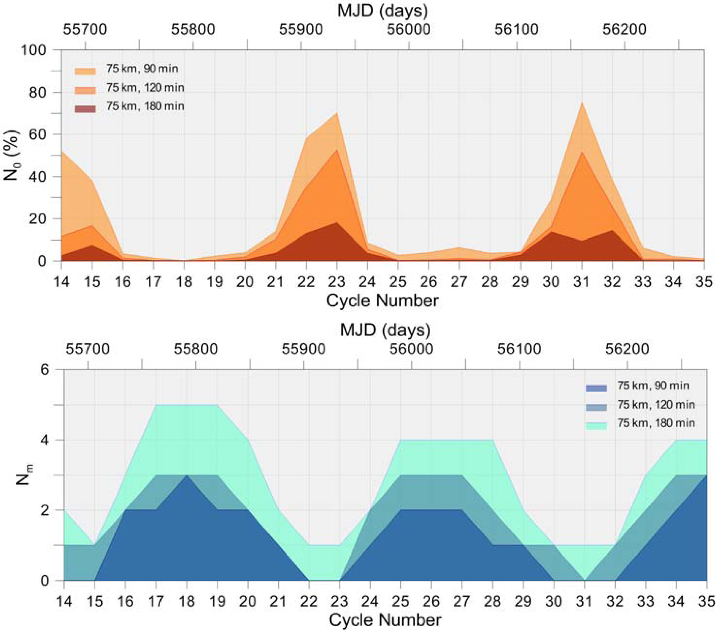
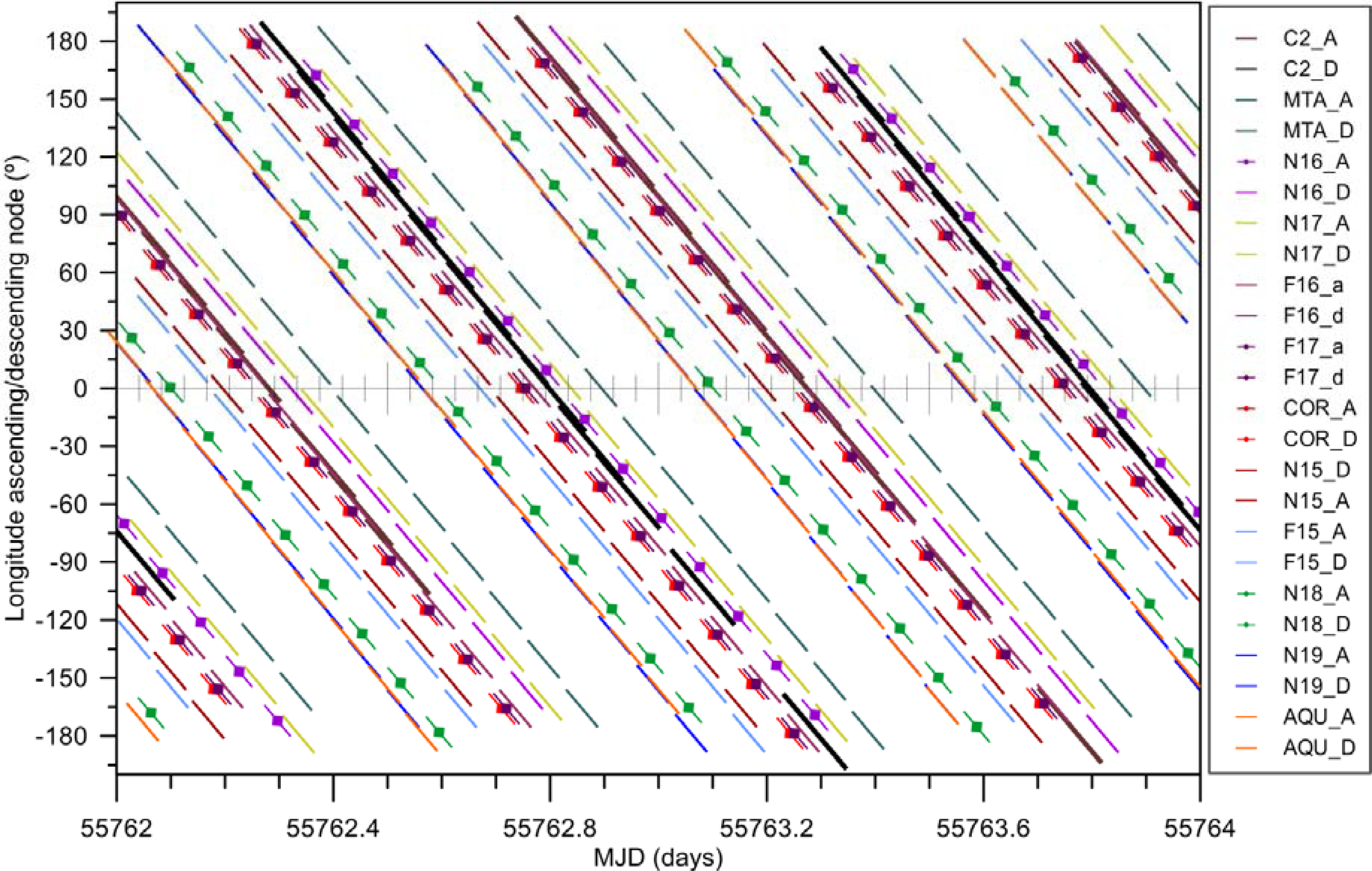
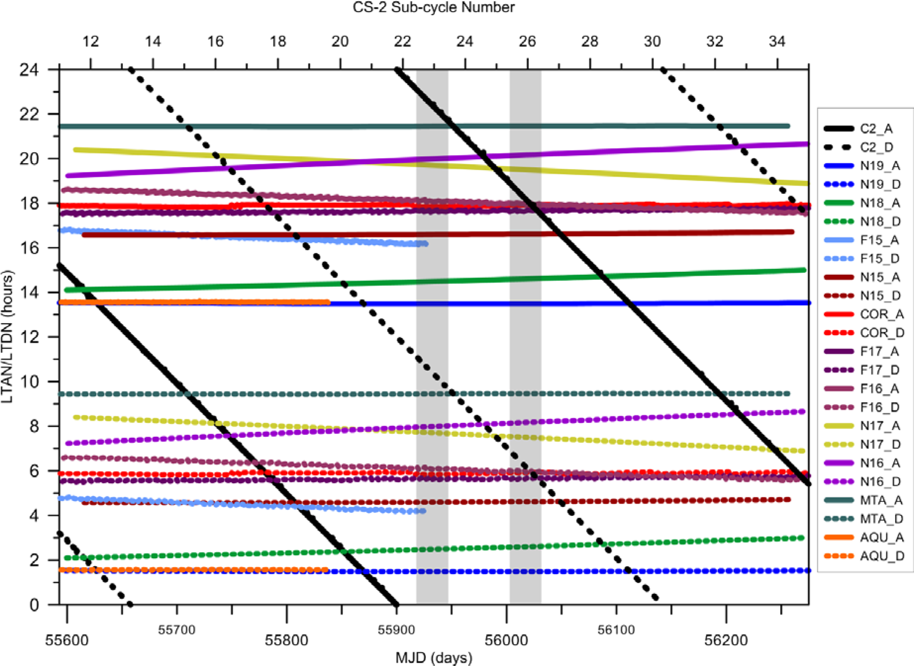
When an ascending CS-2 pass is in phase with an ascending pass of the RS satellite, which is collecting the SI-MWR images, i.e., both satellites have close LTAN and close LTDN, since both passes are nearly parallel. This happens for the middle of CS-2 sub-cycle 26 and satellites Coriolis, F16 and F17 (Figure 7).

(2)

When an ascending CS-2 pass is in phase with a descending pass of the RS satellite, i.e. the CS-2 LTAN is close to the LTDN of the sun-synchronous satellite, or vice versa, when a fraction of the SI-MWR images will be within an acceptable space/time range for the WTC computation. This happens for the middle of CS-2 sub-cycle 18 and satellites Coriolis, F16 and F17 (Figure 7).

Concerning TRMM, since its orbit is not sun-synchronous and with an inclination of 35°, each CS-2 pass will always cross a TRMM pass within two hours, in the latitude band ±40° (Figure 3). Therefore, in this latitude band, a portion of each CS-2 pass will always have TMI images available.

3.3. Spatial and Temporal Coverage with Respect to CryoSat-2

In this section we examine how the space-time coverage of the SI-MWR images varies during the CryoSat-2 mission and how this will affect the WTC estimation for CS-2.

In order to estimate the number of images available for the computation of the WTC for each CS-2 sub-cycle, the number of different images available for each CS-2 point along the satellite track was computed, considering different values for the time difference (ΔT) and distance (ΔD) between each CS-2 point and each image (indeed between the CS-2 point and the closest point in each image) satisfying these conditions.

This is illustrated in Figures 8 and 9 for sub-cycles 23 and 26, respectively, chosen as representative of the extreme conditions that can occur. In this analysis, only one out of every 30 CS-2 points were analyzed (to save computation time) and various values were considered for ΔT and ΔD. For each SI-MWR image, only points with valid TCWV values, according to validity criteria specified by each product, were considered. The results are summarized in

Table 3. Percentage of points with zero available images (N₀) for CryoSat-2 sub-cycle 23 as function of ΔT and ΔD. The main contribution is from five different satellites: MetOp-A, NOAA-16, -17, and -19 and TRMM.

ΔT\ΔD	50 km	75 km	100 km
60 min	65.2	62.5	61.3
90 min	54.0	50.7	49.2
120 min	39.9	36.2	34.6
150 min	24.9	21.3	19.8
180 min	13.6	10.2	9.0

and

Table 4. Percentage of points with zero available images (N₀) for CryoSat-2 sub-cycle 26 as function of ΔT and ΔD. The main contribution is from eight different satellites: NOAA-15, -16, -17, and -19, Coriolis, DMSP-F16 and -F17 and TRMM.

ΔT\ΔD	50 km	75 km	100 km
60 min	8.9	7.2	6.6
90 min	2.9	2.0	1.6
120 min	1.0	0.5	0.3
150 min	0.9	0.4	0.3
180 min	0.8	0.3	0.2

, for sub-cycles 23 and 26, respectively.

Figures 8 and 9 resulting from this analysis show that, as expected, the number of images available for the computation of the WTC increases with latitude, in the same way as the percentage of image overlaps (see Figures 4 and 5). Due to its low inclination, TRMM has a clear impact in the coverage of the low latitudes, in the band ±40 (Figure 3).

As the previous analysis, illustrated by Figures 8 and 9, has shown, the number of images available within a certain time interval is not uniform throughout the year. Sub-cycles 23 (January 2012) and 26 (April 2012) are representative of the less and the most favorable conditions, respectively. Considering these results, the time difference ΔT has a larger effect in the coverage than the distance ΔD. For sub-cycle 26, most of the altimeter ground-track points for which the number of available SI-MWR images is zero (N₀) are either at coastal areas or at high latitudes (Figure 9). Apart from these regions, full coverage is obtained within two hours for this sub-cycle. It can be concluded that the distance ΔD has a clear impact in the coastal regions. Comparing analysis for the same ΔT and different ΔD (not shown here) it can be observed that a decrease in ΔD augments the number of coastal points with no SI-MWR images available. For sub-cycle 23, there are still about 10% of the altimeter ground-track points without any SI-MWR image within range, even when considering a time difference ΔT of three hours.

Having analyzed two sub-cycles representative of the most and less favorable conditions and knowing that the coverage is function of latitude, the percentage of CS-2 points with zero SI-MWR images available (N₀) and the mean number of images available within a certain region (N_m) was computed for two latitude bands: ±5° and in 40°–50°, using ΔD = 75 km and three values for ΔT (90 min, 120 min, and 180 min). Results are illustrated in Figures 10 and 11 respectively.

These figures confirm the results already presented and give a clear indication of the variation of the space-time coverage of the set of SI-MWR images with respect to CS-2. It can be observed that the same conditions repeat every 241 days, the time that takes and ascending/descending CS-2 pass to be in phase with an ascending/descending pass of each sun-synchronous satellite. For example, considering a time interval of three hours both near the equator and at latitude 45°, the percentage of N₀ values varies from 0% to about 15%. In the equator, the mean number of images N_m varies from 0 to 5 while at latitude 45° it varies from 2 to 6. Decreasing the time difference ΔT will change these numbers accordingly. Since the orbital period of each satellite is about 100 min (see Table 2) the critical value for the time difference ΔT is about 120 min. However, for epochs such as for sub-cycle 23, increasing ΔT from 120 min to 180 min considerably increases the number of images available, reducing N₀ from 36% to 10%, for ΔD = 75 km.

In summary, globally the SI-MWR images constitute a very valuable dataset for the WTC computation for CS-2. While for most of the time these images assure a nearly full coverage within three hours, for certain periods of the CS-2 mission the coverage of these images will be insufficient for the computation of an accurate wet tropospheric correction. This stresses the importance of the remaining datasets to be used in the data combination algorithm: GNSS and ERA Interim model derived WTC.

3.4. Sensor Calibration

To prepare the SI-MWR TCWV data from all available MWR imaging sensors for use in the WTC computation, all datasets must be calibrated with respect to a common reference. For this purpose, the WTC retrieved by the Advanced Microwave Radiometer (AMR) on board J2 was used. The reason for adopting AMR is due to the fact that this radiometer has been well monitored and the subject of successive calibrations (e.g., [26]).

Inter-calibration of similar remote sensing instruments on board different missions is a common procedure, and that has been widely used also for microwave radiometers, either as stand-alone methods or as a complement to other approaches, e.g., the use of vicarious targets or comparison with numerical weather models (e.g., [26,27]).

In order to maintain its long-term calibration, AMR on board Jason-2 was subject of a dedicated inter-satellite calibration with respect to Aqua/AMSR-E, TRMM/TMI, and DMSP-F16/SSMIS for a period of three years [26]. In the scope of this inter-calibration process, both latitudinal and different viewing geometry (nadir RA-MWR vs. non-nadir SI-MWR observations) biases were taken into account and corrected for, being the resulting calibrated AMR data and products included on the GDR-D version of the Jason-2 data. An absolute standard is not yet available for microwave radiometers (e.g., [27]), and even though it is known that AMR does have unresolved stability issues and could, therefore, be avoided as a reference, having been carefully recalibrated against reference microwave sensors, makes it itself an acceptable common reference within the present study. In addition, the fact that all altimetric ESA missions fly on sun-synchronous orbits makes it impossible to use their onboard MWR in the calibration of all SI-MWR on board sun-synchronous orbits, due to their different LTAN, being impossible to find collocated measurements between most of these missions. The AMR data used in this study are the GDR-D recently recalibrated products retrieved from RADS.

For the calibration of each SI-MWR derived WTC, a dataset of observations collocated with AMR, i.e., located within a specified space and time interval around the AMR observation, was built. Each collocation is generated by a pair of J2 and SI-MWR sensor observations, providing they occur within 50 km and 45 min of each other. For each AMR ground-track point, the closest SI-MWR image point within the given time interval was selected. In this way, a database of collocations is generated for each MWR imaging sensor.

Using the theory of orbit perturbations, it can be proven that for each RS sun-synchronous satellite (SSat), J2/SSat orbital configurations repeats once every 118 (117.45) days (∼12 J2 cycles). This is illustrated in Figure 12, which represents the time evolution of the LTAN (solid lines) and LTDN (dashed lines) of all sun-synchronous RS satellites and of J2 cycles from middle of J2 cycle 108 (13 June 2011) to middle of J2 cycle 132 (6 February 2012).

Considering that the inclination of each sun-synchronous satellite is greater than 90° and that of J2 is less than 90° (66.4°), the number of J2/SSat collocated points is maximum when an ascending SSat pass is in phase with a descending J2 pass and vice versa, which happens once every 118 days (∼12 J2 cycles). For example, considering Coriolis, this happens for J2 cycles 108, 120, and 132 represented in Figure 12.

For TMI, the J2/TRMM orbital configurations repeat once every 78 (77.76) days (∼ 8 J2 cycles).

To inspect how the calibration parameters depend on the chosen dataset, for Coriolis/WindSat the collocation points and corresponding calibration parameters were computed for a large set of J2 cycles (61 to 156) covering a period of about 2.5 years. It can be observed that the number of collocations and its geographical location has strong time dependence, as already mentioned above. This is well illustrated in Figure 13, in which the location of collocated J2/Coriolis points for three J2 cycles is shown. The time variation of the number of collocated points for J2/AQUA and J2/TRMM was also reported by [26].

The bottom panel of Figure 13 shows (in green) the collocations for J2 cycle 132, for which the time of J2 LTAN coincides with the Coriolis LTDN (see also Figure 12), the most favorable configuration for getting the largest possible number of collocations, spanning the whole latitude range. In this case the passes of both satellites are nearly parallel, although they are moving in opposite ways. The top panel of Figure 13 represents, in blue, the collocations for J2 cycle 138, for which the J2 LTAN coincides with the Coriolis LTAN, that is, the ascending passes of both satellites occur within the accepted time range but they intercept at a large angle, due to the different inclination of the respective orbits. In this case, a considerable number of collocations are obtained but only for the lowest latitudes. Finally, the top panel of the same figure also shows, in red, the collocations for J2 cycle 135. This represents the typical situation for all J2 cycles, which occur between the two configurations described above, in which only a small number of collocations is obtained, all located at high latitudes, therefore sampling only the water vapor conditions of these regions, not representative of the whole range of TCWV values.

The calibration parameters determined for Coriolis/WindSat and each J2 cycle (61 to 156), covering a period of about 2.5 years, were analyzed. It was found that the estimated parameters reveal a small seasonal signal. Therefore, to get stable parameters it is important to use a number of J2 cycles over at least the period of one year, covering the main seasonal variations of the water vapor in the atmosphere.

In summary, for calibration purposes, a set of J2 cycles with a J2/SSat configuration of the first type described above (Figure 13, bottom) shall be selected, covering at least the period of one year.

For each SI-MWR dataset several J2 cycles were selected, separated at intervals of 78 days (for TRMM) and 118 days (for all sun-synchronous satellites), and covering the period of about one year. For example, the set of J2 cycles used in the calibration of Coriolis/WindSat were: 61, 73, 85, and 97.

For all collocated points of the whole set of SI-MWR sensors, the WTC was derived from the TCWV products using (1) the formulation presented by [14], Equation (3), and (2) the formulation proposed by [4], Equation (6). In addition, the WTC from ERA Interim fields was also computed according to Equation (3) for the location and epoch of the collocated points of each database (those of J2). In this way, three WTC datasets were computed. In the subsequent analysis, instead of the negative WTC values, the corresponding symmetric (positive) wet path delay values were used. This approach was adopted to facilitate the illustration of the results both in terms of the calibration plots and associated calibration parameters. The three wet path delays (WPD) datasets calculated this way for each database of collocated points are designated by WPD_Bevis, WPD_Stum, and WPD_ERA, respectively, and were plotted against the corresponding WPD from AMR (WPD_AMR). We recall that WPD_AMR is the symmetric of the WTC correction retrieved from AMR GDR-D products, present in RADS.

For every satellite/sensor, a linear fit was computed for each of the three datasets (WPD_Bevis, WPD_Stum, and WPD_ERA) against WPD_AMR, and the calibration coefficients, i.e., scale factor and offset, were thus derived from the obtained parameters.

Figures 14 and 15 illustrate the results for Coriolis/WindSat images, while Figures 16 and 17 show the corresponding results for MetOp-A/AMSU-A.

Table 5. Calibration parameters (scale factor and offset) of the WPD_Bevis and WPD_Stum with respect to WPD_AMR (linear fits parameters), and RMS of the differences between these datasets before and after calibration.

Satellite	Solution Type	Scale Factor	Offset (cm)	RMS (cm)
				Before	After
AQUA	Bevis	0.980	−0.74	1.41	0.85
	Stum	1.012	−1.01	1.14	0.80
COR	Bevis	0.985	−0.71	1.33	0.88
	Stum	1.016	−0.97	1.11	0.86
F15	Bevis	0.986	−0.63	1.35	1.01
	Stum	1.018	−0.91	1.18	1.01
F16	Bevis	0.985	−0.63	1.34	0.98
	Stum	1.016	−0.89	1.16	0.97
F17	Bevis	0.982	−0.59	1.35	1.01
	Stum	1.012	−0.81	1.17	1.00
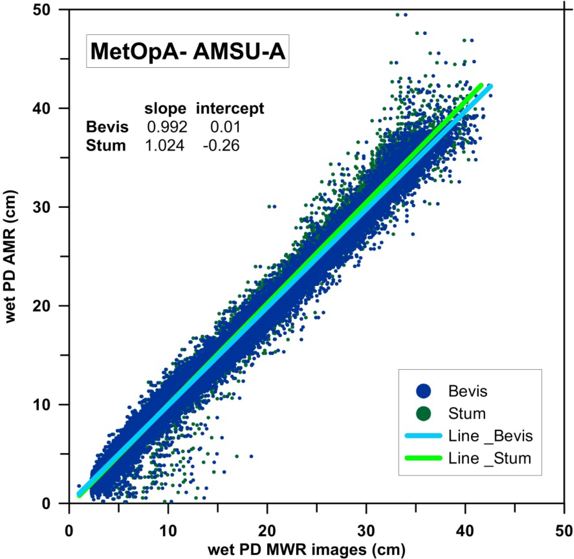
MTA	Bevis	0.992	0.01	1.14	1.13
	Stum	1.024	−0.26	1.09	1.06
N15	Bevis	0.999	0.12	1.22	1,21
	Stum	1.032	−0.18	1.23	1.15
N16	Bevis	0.997	0. 10	1.14	1.14
	Stum	1.029	−0.17	1.14	1.07
N17	Bevis	0.978	0.13	1.24	1.20
	Stum	1.010	−0.14	1.13	1.13
N18	Bevis	0.996	−0.09	1.20	1.19
	Stum	1.029	−0.37	1.13	1.10
N19	Bevis	0.993	0.06	1.17	1.17
	Stum	1.026	−0.21	1.12	1.08
TRM	Bevis	1.004	−0. 93	1. 38	1. 09
	Stum	1.041	−1.40	1.21	1.09

shows the calibration parameters (scale factor and offset) for all 12 analyzed SI-MWR for both WPD_Bevis and WPD_Stum. In addition to the calibration parameters, the statistical parameters of the differences between WPD_AMR and WPD_Bevis or WPD_Stum before and after applying the calibration parameters were computed and are also shown in Table 5.

Results show that, before calibration, WPD_Stum underestimates the wet path delay by 1.0%–4.1% while WPD_Bevis leads to errors in the WPD within [−2.2, +0.4]% (Figures 14 and 17 and Table 5). After calibration, i.e., after applying the derived scale factors and offsets, WPD_Bevis and WPD_Stum agree within ±2 mm.

Figures 15 and 17 illustrate that AMR is well calibrated with respect to ERA Interim and that both the WPD retrieved using the Bevis and Stum approaches agree very well with ERA Interim, although, on average, the calibration coefficients for the Bevis approach are closer to those obtained for ERA Interim (see examples in Figures 15 and 17). It should be recalled that AMR has been calibrated with respect to ECMWF operational model, which, since 2004, is very similar to ERA Interim (see Section 2.3) [26].

Although AMR is well calibrated with respect to ERA Interim, the RMS (Root-Mean Square) of the differences between WPD_AMR and WPD_ERA after calibration has values in the range 1.3–1.6 cm for all satellites, which evidences the lower accuracy of this model when compared to the various SI-MWR. This is also illustrated in Figures 15 and 17, which show a larger spread of WPD_ERA compared to WPD_Bevis, with respect to WPD_AMR.

Results presented in Table 5 show that, overall, all SI‐MWR are well calibrated with respect to AMR. For some of these sensors these results were expected since, as mentioned above, AMR has been calibrated with respect to TMI, AMSR-E and F15-SSM/IS [26].

The fact that the obtained calibration parameters for these satellites are not exactly 1.0 for the scale factor and 0.0 for the offset can be attributed to the following different aspects of the presented methodology: (1) Different datasets for AMSR-E and F15-SSM/IS were used (swath vs. grid products); (2) Possible latitudinal biases were not taken into account; and (3) no restrictions were imposed to, or effect corrected for, the viewing geometry of the SI-MWR observations used, what may help explaining the slight overestimation/underestimation of the SI-MWR-derived WTC using the Bevis and Stum approaches, respectively, before calibration.

The difference between the present results and those presented by [4] for common sensors such as TRMM/TMI and AQUA/AMSR-E can be explained by a set of differences in the two approaches: the comparisons are with respect to two different RA-MWR (JMR vs. AMR); the points used in the calibration were selected for different periods (all Jason-1 cycles spanning a period of only four months in [4]vs. 4 Jason-2 cycles, spanning the period of one year, in this study, chosen to coincide with epochs for which the number of collocations is maximum, covering a larger latitude range; different methods have been used to find the collocated points. In addition, in [4] AMSR-E swath data from CLASS were used while in this paper the corresponding gridded products from RSS were adopted.

For the period of time considered, the best results for RMS of the differences between the WTC derived from AMR and the corresponding values derived from each imaging sensor using the Stum approach and after calibration are (in cm): Coriolis/WindSat (0.80) and AQUA/AMSR-E (0.86). All DMSP satellites’ sensors (F15 (from RSS), F16, and F17) have an RMS of 1.0 cm. For all other sensors (on board TRMM, NOAA-15, -16, -17, -18, -19, MetOp-A, the corresponding RMS with respect to AMR, after calibration, are in the range 1.1–1.2 cm (Table 5). The corresponding RMS differences for the Bevis approach are systematically larger but only by very small values, all less than 1 mm.

In face of these results, WPD_Stum agree with the values derived from AMR slightly better than WPD_Bevis, In practice and for this type of application, the two methods give equivalent results, with differences below the accuracy level of the WTC estimation.

Following the information referred in Section 3.1, the use of DMSP-F15 SSM/I data after August 2006 had to be subject to some prior analysis. Therefore, the latest available version of such data was analyzed, by comparing the derived WTC with that of AMR. Results show that DMSP-F15 SSM/I data from RSS have a performance very similar to those of -F16 and -F17 SSM/IS, being therefore appropriate for use in this study (Table 5). On the contrary, DMSP-F15 SSM/I swath products provided by NOAA CLASS system reveal a serious degradation for that period, evidencing that this dataset has not been corrected for the mentioned anomalies.

The calibration parameters presented in Table 5 refer to wet path delay values. The corresponding parameters to be applied to WTC values are related to those on Table 5 as follows: scale factor—the same; offset—multiply those on Table 5 by (−1).

4. Discussion and Conclusions

This study presented an analysis of the water vapor dataset of SI-MWR sensors available for the computation of the WTC for CryoSat-2, launched in April 2010. In the scope of CP4O project, the next step consists in the implementation of a data combination algorithm (DComb) using, amongst others, the inter-calibrated datasets described in this study.

It is shown that the water vapor dataset of images from MWR on board RS missions constitute a very valuable dataset particularly favorable for CS-2 due to the orbital characteristics of CS-2 and these satellites. Leaving out the AQUA satellite, since AMSR‐E stopped working on October 4, 2011, there are at present 10 RS missions in near polar sun-synchronous orbits providing water vapor products: NOAA-15, -16, -17, -18, -19, MetOp-A, DMSP-F15 (with some restrictions), -F16, -F17, and Coriolis. It is also expected that F18 products shall be released soon. In addition, there is also the low inclination TRMM mission providing measurements in the latitude band ±40°. In summary, since October 2011 there is a total of 11 satellites, with five different MWR scanning sensors with variable pixel size: 50 km, 25 km, and 10 km (for nadir looking).

Results also show that the space-time coverage of these SI-MWR images with respect to CS-2 varies with time, with periods for which there is full coverage within two to three hours, while for less favorable periods, about 10% of the CS-2 measurements over a sub-cycle period will have no images available within three hours (for a distance up to 75 km), thus relying on NWM-derived WTC or the availability of GNSS data near the coast. This stresses the importance of using GNSS data and the best available NWM, which at present and for global studies, is the most recent reanalysis model from ECMWF (ERA Interim).

Coastal regions are of particular importance for CryoSat-2 data, since it is in these regions that the altimeter is operating in the higher resolution in the along-track direction Synthetic Aperture Radar (SAR) mode. In these regions, WTC derived from GNSS data at coastal and island stations shall be used, available online from various networks, e.g., IGS (International GNSS Service), EPN (EUREF Permanent Network), and United States SuomiNet. Details of the GNSS processing and applications to coastal altimetry can be found in [2,3]. It has been shown that the most recent GNSS processing techniques lead to accurate (better than 1 cm) WTC estimates which are stable in time, i.e., show no drift with respect to ERA Interim. The GNSS-derived path delays will be instrumental in the computation of the WTC in the coastal zones, for the full exploitation of the CS-2 SAR measurement mode. In addition, being an independent dataset, in spite of the fact that GNSS measurements are usually not collocated with MWR data, they can play an important role in analyzing the long-term stability of the various radiometers, both RA-MWR and SI-MWR. This shall be a topic for future work.

When using measurements from various instruments, sensor inter-calibration is a crucial step to warrant the consistency of all datasets. To this end, all SI-MWR were calibrated with respect to AMR. It is shown that different approaches for the computation of the WTC from TCWV have an impact in the WTC estimates. Two such approaches were considered here: while the “Bevis approach” leads to WTC with scale factors with respect to AMR in the range 0.98–1.00, the corresponding scale factors for the “Stum approach” are in the range 1.01–1.04. Thus, WTC_Bevis leads to errors in the WPD within [−2, 0] % while WTC_Stum leads to an underestimation by 1%–4%. However, after calibration the WTC derived from both methods are equivalent, with differences within ±2 mm. Results also show that when the two approaches are used to estimate the wet path delay from TCWV or TCWV and T0 values, the difference between the two datasets can be mainly described by a scale factor, that is, WTC_Bevis gives values about 3% larger than WTC_Stum. The pattern of the differences between two datasets of WTC_Bevis and WTC_Stum computed for global ERA Interim grids and for the period of one year (figure not shown) reveals that the RMS differences between the two data sets varies between 0.1 and 1 cm, with a spatial pattern very similar to that shown in Figure 1, that is, strongly correlated with the mean WTC values, thus reinforcing that the main difference between the two methods is a scale factor. Although the two approaches differ in the way they model the water vapor dependence on the temperature, the present results seem to indicate that, regarding this issue, there is no significant difference between the two methods.

In face of the present results, the “Stum approach” allowing the estimation of the WTC directly from TCWV values without any additional information, is the most practical method, particularly for near real time applications. However, a scale factor of 3% in the difference between the values obtained with these two methods gives and error in the WTC up to 1.5 cm, which is not negligible. Therefore, further investigations shall be pursued, by comparisons with other independent data sources such as radiosondes and GNSS to establish which methodology is the most suitable for applications when no calibration is performed.

This study shows that the analyzed dataset of TCWV from SI-MWR sensors is particularly favorable for CS-2 high inclination geodetic orbit. The same does not apply to satellite such as TP, J1, or J2, which are in lower inclination non sun-synchronous orbits and whose tracks have a less favorable relative position with respect to those of the RS sun-synchronous missions. For sun-synchronous altimetric missions such as ERS, Envisat, Altika and Sentinel-3, only a small number of the SI-MWR sensors will be within an acceptable range of their measurements, those whose LTAN are close to the corresponding LTAN of these altimetric missions. In both cases, an improved WTC for these altimetric missions can be obtained from a DComb type of approach using all datasets described in this study, provided the RA-MWR on board each altimetric mission is also incorporated. This DComb type of correction shall be advantageous with respect with the traditional onboard RA-MWR based correction, since a more stable, homogeneous an inter-calibrated WTC will be obtained for all altimetric missions, particularly useful for climate applications.

References and Notes

- Cotton, D.; Benveniste, J.; Clarizia, M.-P.; Roca, M.; Gommenginger, C.; Naeije, M.; Labroue, S.; Picot, N.; Fernandes, J.; Andersen, O.; et al. CryoSat Plus For Oceans: An ESA Project for CryoSat-2 Data Exploitation Over Ocean. Proceedings of EGU General Assembly 2013, Vienna, Austria, 27 April–2 May 2013.
- Fernandes, M.J.; Lazaro, C.; Nunes, A.L.; Pires, N.; Bastos, L.; Mendes, V.B. GNSS-Derived path delay: An approach to compute the wet tropospheric correction for coastal altimetry. IEEE Geosci. Remote Sens. Lett 2010, 7, 596–600. [Google Scholar]
- Fernandes, M.J.; Pires, N.; Lázaro, C.; Nunes, A.L. Tropospheric delays from GNSS for application in coastal altimetry. Adv. Space Res 2013, 51, 1352–1368. [Google Scholar]
- Stum, J.; Sicard, P.; Carrere, L.; Lambin, J. Using objective analysis of scanning radiometer measurements to compute the water vapor path delay for altimetry. IEEE Trans. Geosci. Remote Sens 2011, 49, 3211–3224. [Google Scholar]
- Miller, M.; Buizza, R.; Haseler, J.; Hortal, M.; Janssen, P.; Untch, A. Increased resolution in the ECMWF deterministic and ensemble prediction systems. ECMWF Newslett 2010, 124, 10–16. [Google Scholar]
- Dee, D.P.; Uppala, S.M.; Simmons, A.J.; Berrisford, P.; Poli, P.; Kobayashi, S.; Andrae, U.; Balmaseda, M.A.; Balsamo, G.; Bauer, P.; et al. The ERA-Interim reanalysis: configuration and performance of the data assimilation system. Quart. J. Royal Meteorol. Soc 2011, 137, 553–597. [Google Scholar]
- Eymard, L.; Obligis, E. The Altimetric Wet Troposheric Correction: Progress since the ERS-1 Mission. Proceedings of 15 Years of Progress in Radar Altimetry, Venice, Italy, 13–18 March 2006.
- Brown, S. A novel near-land radiometer wet path-delay retrieval algorithm: Application to the Jason-2/OSTM advanced microwave radiometer. IEEE Trans. Geosci. Remote Sens 2010, 48, 1986–1992. [Google Scholar]
- Tournadre, J. Improved level-3 oceanic rainfall retrieval from dual-frequency spaceborne radar altimeter systems. J.Atmos. Ocean. Technol 2006, 23, 1131–1149. [Google Scholar]
- Tournadre, J.; Lambin-Artru, J.; Steunou, N. Cloud and rain effects on AltiKa/SARAL Ka-band radar altimeter—Part I: Modeling and mean annual data availability. IEEE Trans. Geosci. Remote Sens 2009, 47, 1806–1817. [Google Scholar]
- Verron, J.; Steunou, N. ALTIKA: A Micro-Satellite Ka-band Altimetry Mission. Proceedings of 15 Years Progress in Satellite Altimetry, Venice, Italy, 13–18 March 2006.
- Bevis, M.; Businger, S.; Herring, T.A.; Rocken, C.; Anthes, R.A.; Ware, R.H. GPS meteorology: Remote-sensing of atmospheric water-vapor using the global positioning system. J. Geophys. Res.-Atmos 1992, 97, 15787–15801. [Google Scholar]
- Keihm, S.J.; Janssen, M.A.; Ruf, C.S. TOPEX/Poseidon microwave radiometer (TMR), III, Wet troposphere range correction algorithm and pre-launch error budget. IEEE Trans. Geosci. Remote Sens 1995, 33, 147–161. [Google Scholar]
- Bevis, M.; Businger, S.; Chiswell, S.; Herring, T.A.; Anthes, R.A.; Rocken, C.; Ware, R.H. GPS meteorology—Mapping zenith wet delays onto precipitable water. J.Appl. Meteorol 1994, 33, 379–386. [Google Scholar]
- Mendes, V.B.; Prates, G.; Santos, L.; Langley, R.B. An Evaluation of the Accuracy of Models of the Determination of the Weighted Mean Temperature of the Atmosphere. Proceedings of ION 2000 National Technical Meeting, Anaheim, CA, USA, 26–28 January 2000.
- Mendes, V.B. Modeling the Neutral-Atmosphere Propagation Delay in Radiometric Space Techniques. 1999. [Google Scholar]
- Wang, J.H.; Zhang, L.Y.; Dai, A. Global estimates of water-vapor-weighted mean temperature of the atmosphere for GPS applications. J. Geophys. Res.-Atmos 2005, 110, 1–17. [Google Scholar]
- Ross, R.J.; Rosenfeld, S. Estimating mean weighted temperature of the atmosphere for Global Positioning System applications. J. Geophys. Res.-Atmos 1997, 102, 21719–21730. [Google Scholar]
- Keihm, S.J.; Zlotnicki, V.; Ruf, C.S. TOPEX Microwave radiometer performance evaluation, 1992–1998. IEEE Trans. Geosci. Remote Sens 2000, 38, 1379–1386. [Google Scholar]
- Wentz, F.J. A well-calibrated ocean algorithm for special sensor microwave/imager. J.Geophys. Res.-Ocean 1997, 102, 8703–8718. [Google Scholar]
- Wentz, F.J.; Meissner, T. AMSR Ocean Algorithm, Version 2; Remote Sensing Systems: Santa Rosa, CA, USA, 2000. [Google Scholar]
- Viltard, N.; Burlaud, C.; Kummerow, C.D. Rain retrieval from TMI brightness temperature measurements using a TRMM PR-based database. J. Appl. Meteorol. Clim 2006, 45, 455–466. [Google Scholar]
- Meissner, T.; Wentz, F. Ocean Retrievals for WindSat—Radiative Transfer Model, Algorithm, Validation. Proceedings of OCEANS 2005 MTS/IEEE, Washington, DC, USA, 18–23 September 2005.
- Weng, F.; Ferraro, R.R.; Grody, N.C. Effects of AMSU Cross-Scan Asymmetry of Brightness Temperatures on Retrieval of Atmospheric and Surface Parameters. In Microwave Radiometry & Remote Sensing of the Earth’s Surface and Atmosphere; Pampaloni, P., Paloscia, S., Eds.; VSP: Leiden, The Netherlands, 2000; pp. 255–262. [Google Scholar]
- Ignatov, A.; Laszlo, I.; Harrod, E.D.; Kidwell, K.B.; Goodrum, G.P. Equator crossing times for NOAA, ERS and EOS sun-synchronous satellites. Int. J. Remote Sens 2004, 25, 5255–5266. [Google Scholar]
- Brown, S. Maintaining the long-term calibration of the Jason-2/OSTM advanced microwave radiometer through intersatellite calibration. IEEE Trans. Geosci. Remote Sens 2013, 51, 1531–1543. [Google Scholar]
- Cao, C.Y.; Chen, R.Y.; Miller, L. Monitoring the Jason-2/AMR stability using SNO observations from AMSU on MetOp-A. Mar. Geod 2011, 34, 431–446. [Google Scholar]