Assessing Water Stress of Desert Tamarugo Trees Using in situ Data and Very High Spatial Resolution Remote Sensing

 ,
,
Abstract
:
1. Introduction
- Test the water stress indicators proposed by Chávez et al. [8] for Tamarugo plants under laboratory conditions, namely canopy water content and leaf area index, on single Tamarugo trees under different field water stress scenarios.
- Test the vegetation indices proposed by Chávez et al. [8] to assess water condition of single Tamarugo trees by using the spectral bands of WorldView2 images and in situ measurements.
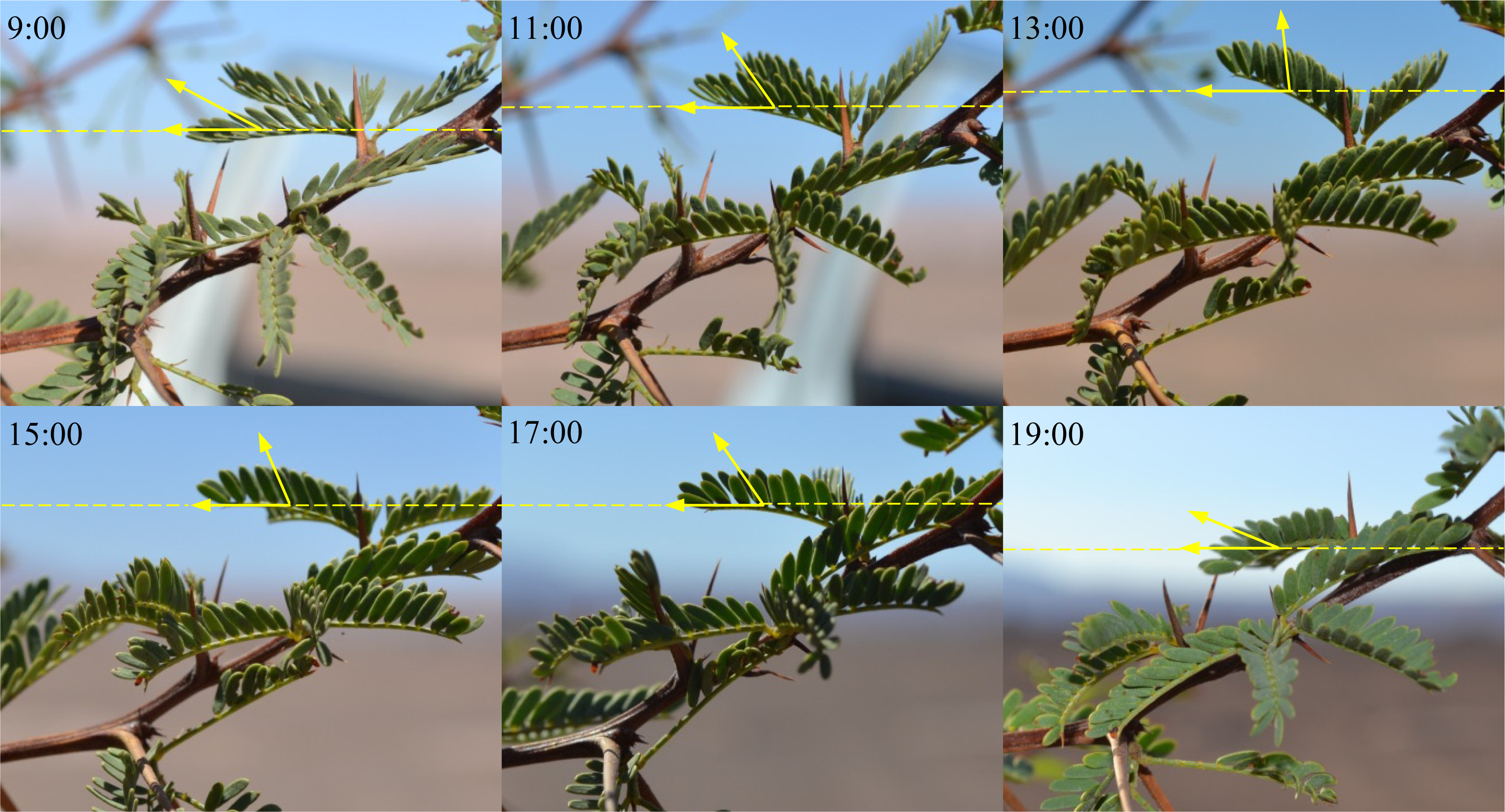
- Study Tamarugo leaf movements during the day in the field and their implications for remote sensing based estimations of water stress.
2. Material and Methods
2.1. Species Description
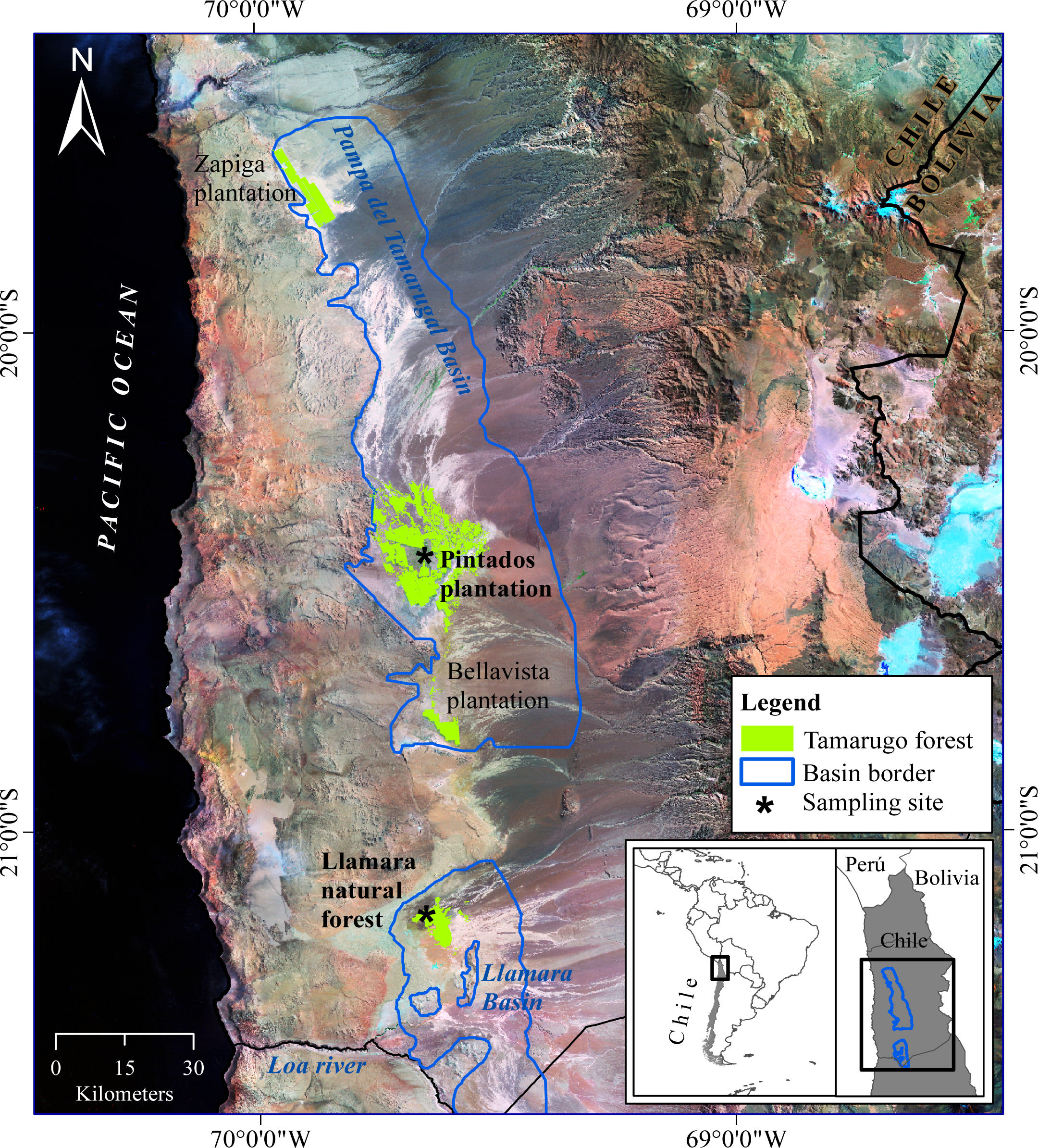
2.2. Study Area
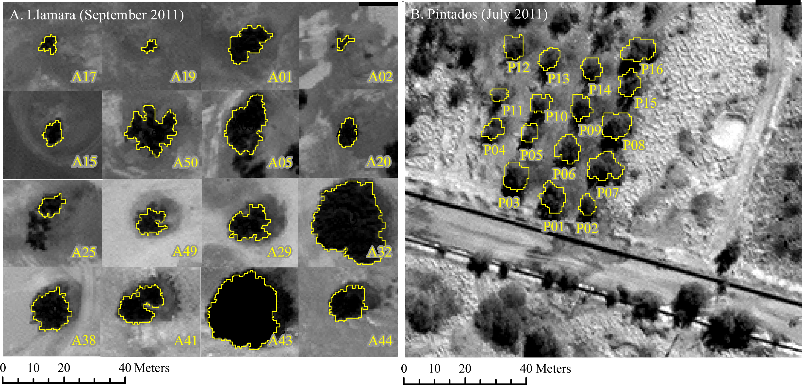
2.2.1. Llamara Site
2.2.2. Pintados Site
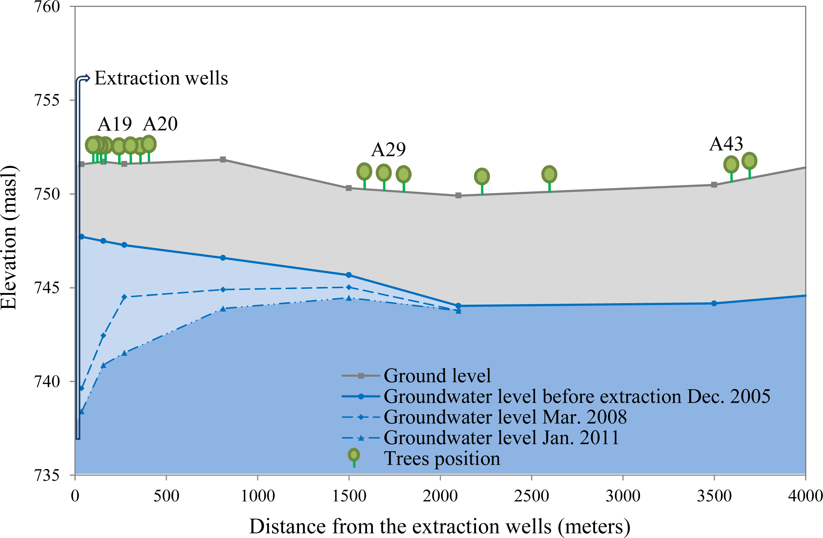
2.3. Groundwater Depletion Scenarios
- Null water depletion (Dep1-null): trees located in the Llamara site at a distance >1500 m from the pumping area (nine trees). Ground water depth was between 5 and 6 m in January 2011 (Figure 2).
- Short-term intensive water depletion (Dep2-int): trees located at the Llamara site at a distance <500 m from the pumping area with depletions of around 6–7 m in five years (seven trees). Ground water depth was between 10 and 12 m in January 2011 (Figure 2).
- Long-term gradual water depletion (Dep3-grad): trees located at the Pintados site with depletions of around 1 meter in 20 years (16 trees). At this site groundwater depth was about 11 m in 2011 according to the records of the closest DGA (Chilean Water Service) monitoring well (about 1 km away from this site).
2.4. In Situ Measurements
2.5. Calculation of Spectral Vegetation Indices using Object-Based Analysis and WorldView2 Images
2.5.1. The WorldView2 Sensor
2.5.2. Crown Delineation
2.5.3. Vegetation Indices
2.6. Data Analysis
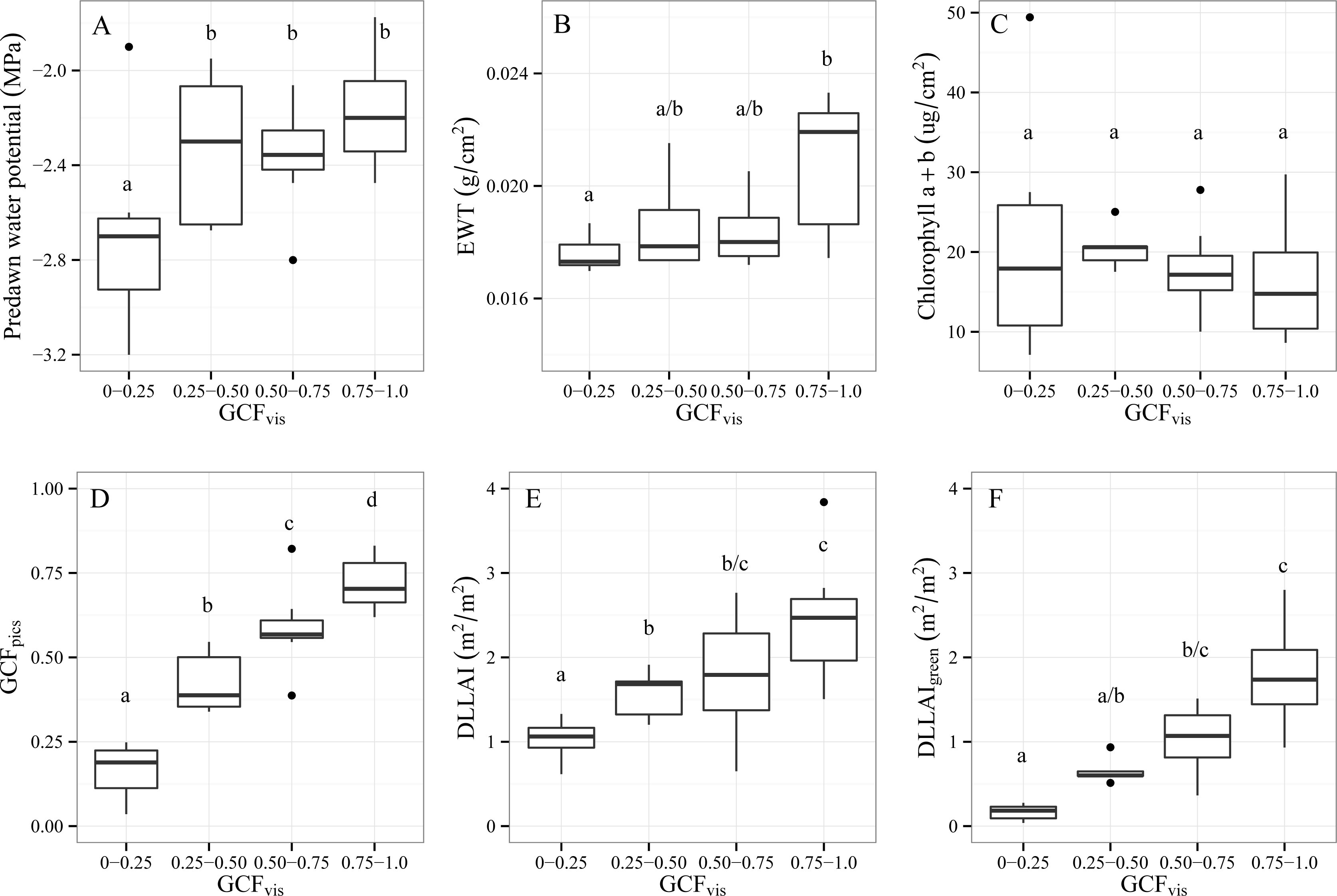
- Objective 1. Test the variables CWC and LAI as water stress indicators for single Tamarugo trees under different field water stress scenarios. We tested first for significant differences in predawn water potential between trees under the three depletion scenarios to check if they were facing different levels of water stress. Then we tested for significant differences in selected foliar and canopy variables between trees under different depletion scenarios. Additionally, we analyzed whether trees with a different GCFvis were significantly different in terms of predawn water potential, foliar biochemistry and other canopy variables. Significance was tested with the Tukey-Kramer multiple comparison test for unbalanced samples with a significance level α of 0.05.
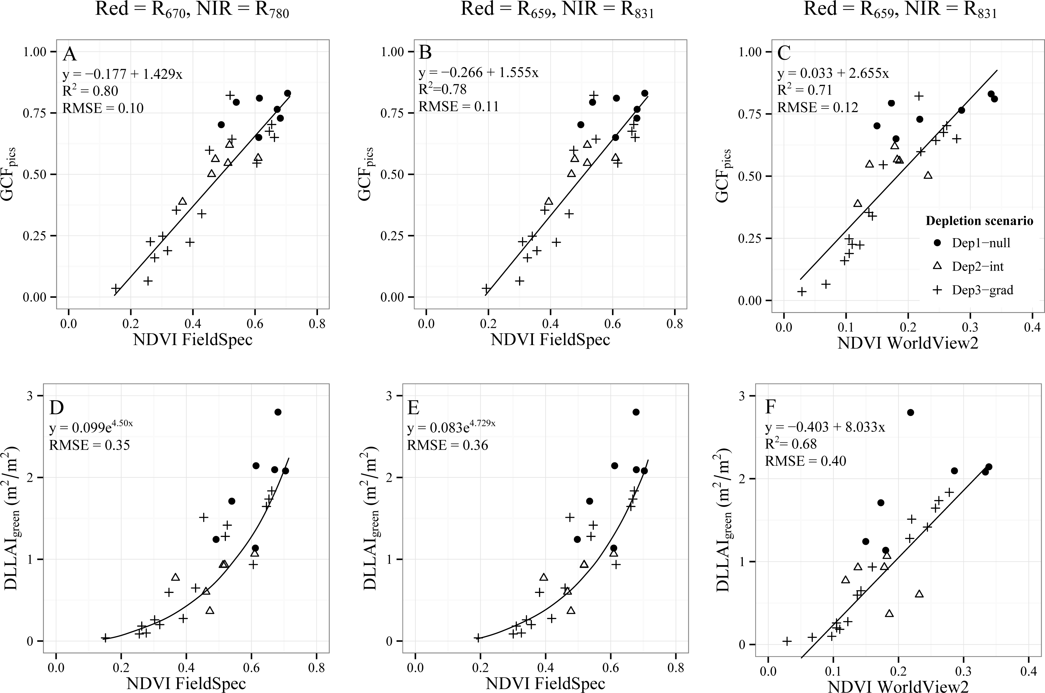
- Objective 2. Test the CIRed-edge and NDVI to assess water condition of single Tamarugo trees by using WorldView2 images and in situ measurements. We tested the capability of these two vegetation indices as best field water stress indicators using the root mean squared errors (RMSE) between estimated values and the in situ measurements. We compared the fitted curves and RMSE for the indices calculated using FieldSpec data, which were obtained during the field campaign, and the indices calculated from satellite data to check for seasonal effects in the remote sensing estimations.
- Objective 3. Study Tamarugo leaf movements during the day in the field and their implications for remote sensing based estimations of water stress. The photographic recording of diurnal leaf movements was carried out simultaneously with the FieldSpec measurements, and therefore, diurnal changes in canopy reflection can be associated to these movements. Using the hourly FieldSpec data, we obtained hourly values of CIRed-edge and NDVI and calculated the correlation coefficient (R) between these values and hourly values of solar radiation. We hypothesize that solar radiation is the main environmental variable driving the leaf movements of Tamarugo trees since this has been shown for other Leguminosae plants [38–40]. Solar radiation data were obtained from the meteorological station Canchones of the Universidad Arturo Prat (20°26′36″S, 69°41′43″W). A potential correlation between spectral vegetation indices and solar radiation would imply that not only diurnal but also seasonal changes of this variable would have an impact on biophysical retrievals from remote sensing data. This is especially relevant for hyper-arid ecosystems such as the Atacama Desert, where the solar radiation can be extremely high with high fluctuations between summer and winter [41,42].
3. Results
3.1. Biophysical Response of the Tamarugo Trees under Different Water Depletion Scenarios
3.1.1. Differences between Depletion Scenarios
3.1.2. Differences between GCFvis Classes
3.2. Remote Sensing Based Estimations of Tamarugo Water Status
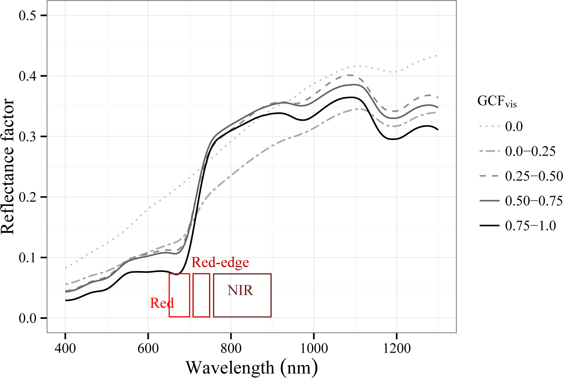
3.2.1. Spectral Response to Green Foliage Loss
3.2.2. Vegetation Indices for GCF and DLLAIgreen Estimations
3.2.2.1. Normalized Difference Vegetation Index (NDVI)
3.2.2.2. Red-edge Chlorophyll Index (CIRed-edge)
3.3. Effects of Tamarugo Pulvinar Movements on Spectral Reflectance
4. Discussion
5. Conclusions and Recommendations
Acknowledgments
Conflict of Interest
References
- Ezcurra, E. Global Deserts Outlook; United Nations Environment Programme: Nairobi, Kenya, 2006. [Google Scholar]
- Blaschke, T. Object based image analysis for remote sensing. ISPRS J Photogram. Remote Sens 2010, 65, 2–16. [Google Scholar]
- Laliberte, A.S.; Rango, A.; Havstad, K.M.; Paris, J.F.; Beck, R.F.; McNeely, R.; Gonzalez, A.L. Object-oriented image analysis for mapping shrub encroachment from 1937 to 2003 in southern New Mexico. Remote Sens. Environ 2004, 93, 198–210. [Google Scholar]
- Laliberte, A.S.; Fredrickson, E.L.; Rango, A. Combining decision trees with hierarchical object-oriented image analysis for mapping arid rangelands. Photogram. Eng. Remote Sens 2007, 73, 197–207. [Google Scholar]
- Gibbes, C.; Adhikari, S.; Rostant, L.; Southworth, J.; Qiu, Y. Application of object based classification and high resolution satellite imagery for savanna ecosystem analysis. Remote Sens 2010, 2, 2748–2772. [Google Scholar]
- Asner, G.P.; Wessman, C.A.; Bateson, C.A.; Privette, J.L. Impact of tissue, canopy, and landscape factors on the hyperspectral reflectance variability of arid ecosystems. Remote Sens. Environ 2000, 74, 69–84. [Google Scholar]
- Borzuchowski, J.; Schulz, K. Retrieval of leaf area index (LAI) and soil water content (WC) using hyperspectral remote sensing under controlled glass house conditions for spring barley and sugar beet. Remote Sens 2010, 2, 1702–1721. [Google Scholar]
- Chávez, R.O.; Clevers, J.G.P.W.; Herold, M.; Ortiz, M.; Acevedo, E. Modelling the spectral response of the desert tree Prosopis tamarugo to water stress. Int. J. Appl. Earth Obs. Geoinf 2013, 21, 53–65. [Google Scholar]
- Taiz, L.; Zeiger, E. Plant Physiology; Sinauer Associates: Sunderland, MA, USA, 2010. [Google Scholar]
- Kimes, D.S.; Kirchner, J.A. Diurnal variations of vegetation canopy structure. Int. J. Remote Sens 1983, 4, 257–271. [Google Scholar]
- Moran, M.S.; Pinter, P.J., Jr; Clothier, B.E.; Allen, S.G. Effect of water stress on the canopy architecture and spectral indices of irrigated alfalfa. Remote Sens. Environ 1989, 29, 251–261. [Google Scholar]
- Verhoef, W.; Bach, H. Coupled soil-leaf-canopy and atmosphere radiative transfer modeling to simulate hyperspectral multi-angular surface reflectance and TOA radiance data. Remote Sens. Environ 2007, 109, 166–182. [Google Scholar]
- Rojas, R.; Dassargues, A. Groundwater flow modelling of the regional aquifer of the Pampa del Tamarugal, Northern Chile. Hydrogeol. J 2007, 15, 537–551. [Google Scholar]
- Romero, H.; Méndez, M.; Smith, P. Mining development and environmental injustice in the Atacama Desert of Northern Chile. Environ. Justice 2012, 5, 70–76. [Google Scholar]
- Gajardo, R. La Vegetación Natural de Chile Clasificación y Distribución Geográfica; Editorial Universitaria: Santiago, Chile, 1994. [Google Scholar]
- CONAMA, Biodiversidad de Chile, Patrimonio Y Desafíos; Ocho Libros Editores: Santiago, Chile, 2008.
- CONAF, Plan de Manejo Reserva Nacional Pampa del Tamarugal; Corporación Nacional Forestal (CONAF); Ministerio de Agricultura: Gobierno, Chile, 1997; p. 110.
- Estades, C.F. Natural history and conservation status of the Tamarugo Conebill in northern Chile. Wilson Bull 1996, 108, 268–279. [Google Scholar]
- Ramírez-Leyton, G.; Pincheira-Donoso, D. Fauna del Altiplano y Desierto de Atacama. Vertebrados de la Provncia de El Loa; Phrynosaura Ediciones: Calama, Chile, 2005. [Google Scholar]
- Oyarzún, J.; Oyarzún, R. Sustainable development threats, inter-sector conflicts and environmental policy requirements in the arid, mining rich, Northern Chile territory. Sustain. Dev 2011, 19, 263–274. [Google Scholar]
- Burkart, A. A monograph of the genus Prosopis (Leguminosae subfam. Mimosoideae). J. Arnold. Arbor 1976, 57, 219–249. [Google Scholar]
- Altamirano, H. Prosopis tamarugo Phil. Tamarugo. In Las especies arbóreas de los bosques templados de Chile y Argentina. Autoecología; Donoso, C., Ed.; Marisa Cuneo Ediciones: Valdivia, Chile, 2006; pp. 534–540. [Google Scholar]
- Riedemann, P.; Aldunate, G.; Teillier, S. Flora nativa de valor ornamental. Chile, Zona Norte. Identificación y propagación; Productora Gráfica Andros Ltda: Santiago, Chile, 2006; p. 404. [Google Scholar]
- Acevedo, E.; Ortiz, M.; Franck, N.; Sanguineti, P. Relaciones hídricas de Prosopis tamarugo Phil. Uso de isótopos estables; Universidad de Chile: Santiago, Chile, 2007; p. 82. [Google Scholar]
- Sudzuki, F. Environmental Influence on Foliar Anatomy of Prosopis Tamarugo Phil. In The Current State of Knowledge on Prosopis Tamarugo; Habit, M., Ed.; FAO: Rome, Italy, 1985. [Google Scholar]
- DICTUC, Anexo VIII.2 Modelación de la Evolución del Nivel de la Napa en la Pampa del Tamarugal. In EIA proyecto Pampa Hermosa; Dirección de Investigaciones Científicas y Tecnológicas Universidad Católica de Chile: Santiago, Chile, 2008; p. 169.
- Geohidrología-SQM, Informe Semestral 2. In Plan de Segumiento Ambiental Hidrogeológico Proyecto Pampa Hermosa; Geohidrología: Santiago, Chile, 2012; p. 118.
- Meyer, W.S.; Ritchie, J.T. Resistance to water flow in the Sorghum plant. Plant. Physiol 1980, 65, 33–39. [Google Scholar]
- Scholander, P.F.; Hammel, H.T.; Bradstreet, E.D.; Hemmingsen, E.A. Sap pressure in vascular plants. Science 1965, 148, 339–346. [Google Scholar]
- Lichtenthaler, H.K.; Wellburn, A.R. Determination of total carotenoids and chlorophyll a and b of leaf extract in different solvents. Biochem. Soc. Trans. 1983, 591–592. [Google Scholar]
- LI-COR, LAI-2000 Plant Canopy Analyser. Instruction Manual; LICOR: Lincoln, NE, USA, 1992.
- Jonckheere, I.; Fleck, S.; Nackaerts, K.; Muys, B.; Coppin, P.; Weiss, M.; Baret, F. Review of methods for in situ leaf area index determination: Part I. Theories, sensors and hemispherical photography. Agric. For. Meteorol 2004, 121, 19–35. [Google Scholar]
- Peper, P.J.; McPherson, E.G. Evaluation of four methods for estimating leaf area of isolated trees. Urban. For. Urban. Green 2003, 2, 19–29. [Google Scholar]
- Ortiz, M.; Silva, P.; Acevedo, E. Leaf Water Parameters in Prosopis Tamarugo Phil. Subject to a Lowering of the Water Table. In Nivel freático en la Pampa del Tamarugal y Crecimiento de Prosopis tamarugo Phil; Tesis para optar al Grado Académico de Doctor en Ciencias Silvoagrpecuarias y Veterinarias: Santiago, Chile, 2010; pp. 15–42. [Google Scholar]
- Updike, T.; Comp, C. Radiometric Use of WorldView2 Imagery; Technical Note; Revision 1; DigitalGlobe, Inc.: Longmont, CO, USA, 2010; p. 17. [Google Scholar]
- Tucker, C.J. Red and photographic infrared linear combinations for monitoring vegetation. Remote Sens. Environ 1979, 8, 127–150. [Google Scholar]
- Gitelson, A.A.; Keydan, G.P.; Merzlyak, M.N. Three-band model for noninvasive estimation of chlorophyll, carotenoids, and anthocyanin contents in higher plant leaves. Geophys. Res. Lett 2006, 33, L11402. [Google Scholar]
- Pastenes, C.; Pimentel, P.; Lillo, J. Leaf movements and photoinhibition in relation to water stress in field-grown beans. J. Exp. Bot 2005, 56, 425–433. [Google Scholar]
- Liu, C.C.; Welham, C.V.J.; Zhang, X.Q.; Wang, R.Q. Leaflet movement of Robinia pseudoacacia in response to a changing light environment. J. Integr. Plant. Biol 2007, 49, 419–424. [Google Scholar]
- Pastenes, C.; Porter, V.; Baginsky, C.; Norton, P.; González, J. Paraheliotropism can protect water-stressed bean (Phaseolus vulgaris L.) plants against photoinhibition. J. Plant. Physiol 2004, 161, 1315–1323. [Google Scholar]
- Ortega, A.; Escobar, R.; Colle, S.; de Abreu, S.L. The state of solar energy resource assessment in Chile. Renewable Energy 2010, 35, 2514–2524. [Google Scholar]
- Hirschmann, R.J. Records on solar radiation in Chile. Solar Energy 1973, 14, 129–138. [Google Scholar]
- Schmidhalter, U. The gradient between pre-dawn rhizoplane and bulk soil matric potentials, and its relation to the pre-dawn root and leaf water potentials of four species. Plant. Cell. Environ 1997, 20, 953–960. [Google Scholar]
- Veste, M.; Staudinger, M.; Küppers, M. Spatial and temporal variability of soil water in drylands: Plant water potential as a diagnostic tool. Forestry Studies China 2008, 10, 74–80. [Google Scholar]
- Richter, H. Water relations of plants in the field: some comments on the measurement of selected parameters. J. Exp. Bot 1997, 48, 1–7. [Google Scholar]
- Boochs, F.; Kupfer, G.; Dockter, K.; Kuhbauch, W. Shape of the red edge as vitality indicator for plants. Int. J. Remote Sens 1990, 11, 1741–1753. [Google Scholar]
- Filella, I.; Penuelas, J. The red edge position and shape as indicators of plant chlorophyll content, biomass and hydric status. Int. J. Remote Sens 1994, 15, 1459–1470. [Google Scholar]
- Horler, D.N.H.; Dockray, M.; Barber, J. The red edge of plant leaf reflectance. Int. J. Remote Sens 1983, 4, 273–288. [Google Scholar]
- Carter, G.A.; Knapp, A.K. Leaf optical properties in higher plants: linking spectral characteristics to stress and chlorophyll concentration. Am. J. Bot 2001, 88, 677–684. [Google Scholar]
- Malenovský, Z.; Bartholomeus, H.M.; Acerbi-Junior, F.W.; Schopfer, J.T.; Painter, T.H.; Epema, G.F.; Bregt, A.K. Scaling dimensions in spectroscopy of soil and vegetation. Int. J. Appl. Earth Obs. Geoinf 2007, 9, 137–164. [Google Scholar]
- Moorthy, I.; Miller, J.R.; Noland, T.L. Estimating chlorophyll concentration in conifer needles with hyperspectral data: An assessment at the needle and canopy level. Remote Sens. Environ 2008, 112, 2824–2838. [Google Scholar]
- Baret, F.; de Solan, B.; Lopez-Lozano, R.; Ma, K.; Weiss, M. GAI estimates of row crops from downward looking digital photos taken perpendicular to rows at 57.5° zenith angle: Theoretical considerations based on 3D architecture models and application to wheat crops. Agric. For. Meteorol 2010, 150, 1393–1401. [Google Scholar]
- Liu, J.; Pattey, E.; Admiral, S. Assessment of in situ crop LAI measurement using unidirectional view digital photography. Agric. For. Meteorol 2013, 169, 25–34. [Google Scholar]


| Field Campaign/WorldView2 Image | Variables | Sample and Location | Dates |
|---|---|---|---|
| Field campaign summer 2011 | Hydraulic, biochemical and structural variables | 32 trees (16 Llamara, 16 Pintados) | 24–28/01/2011 |
| Canopy spectral reflectance at midday (FieldSpec) | 32 trees (16 Llamara, 16 Pintados) × 4 quarters per tree = 128 measurements | 24–28/01/2011 | |
| Field campaign summer 2012 | Diurnal leaf movements and canopy spectral reflectance (FieldSpec) | 3 trees (Llamara) | 13–15/01/2012 |
| WorldView2 image winter 2011 | Top-of-atmosphere (TOA) spectral reflectance | 1 scene (Pintados) | 13/07/2011 |
| WorldView2 image spring 2011 | Top-of-atmosphere (TOA) spectral reflectance | 1 scene (Llamara) | 25/09/2011 |
| Variables | Units | Sampling Time | Sampling Scheme | Instrument/Procedure | Reference/Formula |
|---|---|---|---|---|---|
| Hydraulic | |||||
| Leaf water potential | MPa | Predawn | 4 twigs per tree | Scholander chamber | [28,29] |
| Foliar biochemistry | |||||
| Equivalent water thickness (EWT) | g/cm2 | Midday | 4 twigs per tree | Precision weight (0.0001 g) and oven | |
| Canopy water content (CWC) | g/cm2 | CWC = EWT × DLLAIgreen | |||
| Chlorophyll (a + b) and Carotenoids | μg/cm2 | Midday | 4 twigs per tree | Spectro-photometric analysis of extracts dissolved in 80% acetone | [30] |
| Canopy structure | |||||
| Green canopy fraction visual estimation(GCFvis) | Any time | 2 times, 2 surveyors | Visual estimation, using five categories: 0; 0.01–0.25; 0.25–0.50; 0.50–0.75; 0.75–1.0 | ||
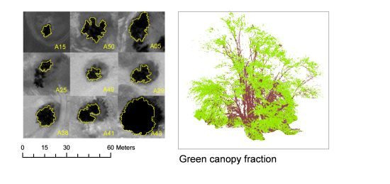
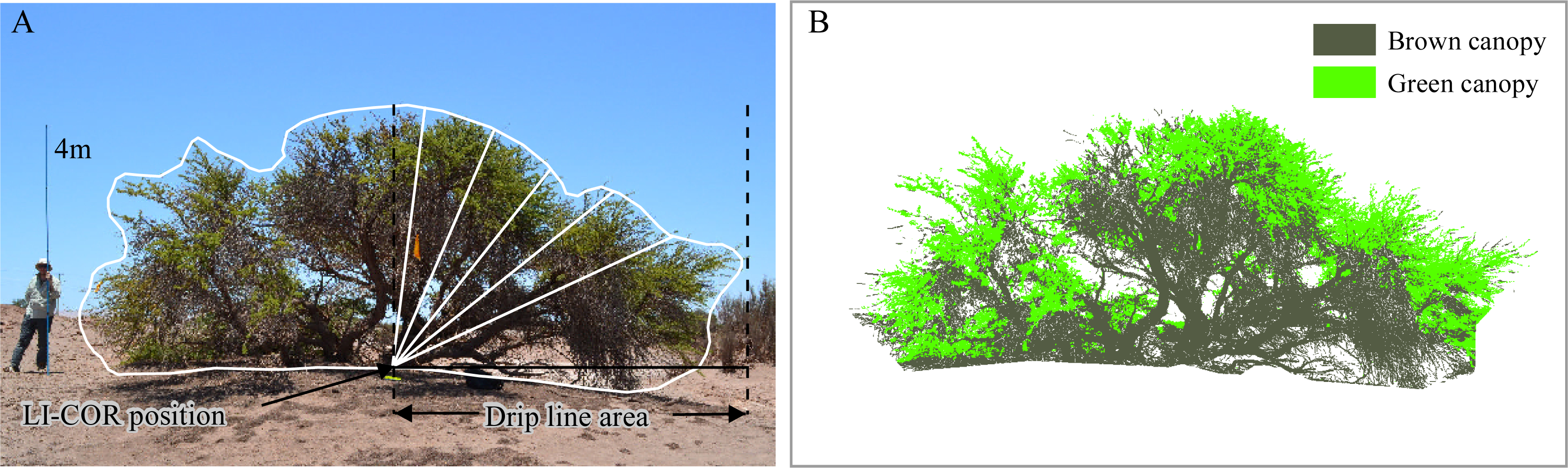
| Green canopy fraction from digital pictures (GCFpics) | Any time | 2 digital color pictures (RGB) per tree | Object-based image analysis. Segmentation: multiresolution (scale: 10, shape: 0.5, compactness: 0.1). Classification: objects with [G/(R + G + B) > 0.34] as green canopy; objects with [R/(R + G + B) > 0.37] as brown canopy. | ||
| Drip line leaf area index (DLLAI) (green + brown) | m2/m2 | Dawn or sunset | 4 partial records (at each tree quarters) | LI-COR LAI-2000 instrument. Measurements corrected by the tree profile | [31,32,33] |
| Green drip line leaf area index (DLLAIgreen) | m2/m2 | DLLAIgreen = DLLAI × GCFpics | |||
| Remote Sensing Feature | Formula Using the Position of the WorldView2 Spectral Bands (nm) |
|---|---|
| Normalized Difference Vegetation Index (NDVI) [36] | (R831 − R659)/(R831 + R659) |
| Red-edge Chlorophyll Index (CIRed-edge) [37] | R831/R724 − 1 |
| Variables | Depletion Scenarios | ||
|---|---|---|---|
| Dep1-Null | Dep2-Intensive (6–7 m in 5 years) | Dep3-Gradual (1 m in 20 years) | |
| Hydraulic | |||
| Predawn leaf water potential (MPa) | −2.061 (0.199) a | −2.194 (0.164) a | −2.588 (0.316) b |
| Biochemistry | |||
| EWT (g/cm2) | 0.021 (0.002) a | 0.019 (0.002) b | 0.018 (0.002) b |
| Chlorophyll (a + b) (μg/cm2) | 12.28 (4.08) a | 18.55 (2.05) a/b | 19.23 (7.31) b |
| Carotenoids (μg/cm2) | 475.9 (115.9) a | 620.7 (46.5) a/b | 761.7 (236.8) b |
| Structure | |||
| DLLAI (m2/m2) | 2.486 (0.718) a | 1.482 (0.664) b | 1.658 (0.677) b |
| GCFpics | 0.755 (0.064) a | 0.517(0.086) b | 0.405 (0.253) b |
| DLLAIgreen | 1.887 (0.576) a | 0.743 (0.286) b | 0.797 (0.671) b |
| Crown area (m2) | 200.7 (175.0) a | 69.6 (65.2) b | 46.0 (17.13) b |
© 2013 by the authors; licensee MDPI, Basel, Switzerland This article is an open access article distributed under the terms and conditions of the Creative Commons Attribution license ( http://creativecommons.org/licenses/by/3.0/).
Share and Cite
Chávez, R.O.; Clevers, J.G.P.W.; Herold, M.; Acevedo, E.; Ortiz, M. Assessing Water Stress of Desert Tamarugo Trees Using in situ Data and Very High Spatial Resolution Remote Sensing. Remote Sens. 2013, 5, 5064-5088. https://doi.org/10.3390/rs5105064
Chávez RO, Clevers JGPW, Herold M, Acevedo E, Ortiz M. Assessing Water Stress of Desert Tamarugo Trees Using in situ Data and Very High Spatial Resolution Remote Sensing. Remote Sensing. 2013; 5(10):5064-5088. https://doi.org/10.3390/rs5105064
Chicago/Turabian StyleChávez, Roberto O., Jan G. P. W. Clevers, Martin Herold, Edmundo Acevedo, and Mauricio Ortiz. 2013. "Assessing Water Stress of Desert Tamarugo Trees Using in situ Data and Very High Spatial Resolution Remote Sensing" Remote Sensing 5, no. 10: 5064-5088. https://doi.org/10.3390/rs5105064