A Joint Land Cover Mapping and Image Registration Algorithm Based on a Markov Random Field Model

Abstract

Traditionally, image registration of multi-modal and multi-temporal images is performed satisfactorily before land cover mapping. However, since multi-modal and multi-temporal images are likely to be obtained from different satellite platforms and/or acquired at different times, perfect alignment is very difficult to achieve. As a result, a proper land cover mapping algorithm must be able to correct registration errors as well as perform an accurate classification. In this paper, we propose a joint classification and registration technique based on a Markov random field (MRF) model to simultaneously align two or more images and obtain a land cover map (LCM) of the scene. The expectation maximization (EM) algorithm is employed to solve the joint image classification and registration problem by iteratively estimating the map parameters and approximate posterior probabilities. Then, the maximum a posteriori (MAP) criterion is used to produce an optimum land cover map. We conducted experiments on a set of four simulated images and one pair of remotely sensed images to investigate the effectiveness and robustness of the proposed algorithm. Our results show that, with proper selection of a critical MRF parameter, the resulting LCMs derived from an unregistered image pair can achieve an accuracy that is as high as when images are perfectly aligned. Furthermore, the registration error can be greatly reduced.

1. Introduction

Remotely sensed images captured from satellites have been widely used for land cover mapping applications because of their capability to allow classification of different land cover types without having to physically assess the area of interest. In a situation where a single image does not provide sufficient classification performance, integrating multiple images of the same area is a common practice to increase the discrimination capability. Some applications, especially agricultural field mapping, particularly benefit from using multitemporal sequences of satellite images because vegetation appearance often changes according to the season. Moreover, multiple input images from different satellites can be used to further improve classification performance by providing better spectral separation characteristics that a single sensor alone cannot provide. A practical application is reported in [1] where multi-temporal sequences of synthetic aperture radar (SAR) images and a single optical image were used. The results from this study showed that the overall discrimination performance was increased, consistent with other similar research where multi-sensor data have been combined. Skriver et al. [2] emphasized the benefits of using multi-temporal SAR images in short succession (weekly to monthly acquisitions) for crop classification. These authors reported improved classification accuracy by using multi-temporal information. The authors in [3] exploited the crop phenology information to determine the growth stages by using multi-temporal TerraSAR-X, ASAR/ENVISAT and PALSAR/ALOS images. They reported a significant correlation between backscattering coefficient and the normalized vegetation index obtained from SPOT4-5 images. Similarly, the work in [4] used multitemporal remote sensing data for yield estimation of wheat.

The problems of multisource and multitemporal land cover mapping have been extensively studied in [5–7]. In [5], the authors modeled the multisource and multitemporal images to have the MRF properties, and used this model to develop an image classification algorithm for remote sensing images. Thoonen et al. in [6] attempted to jointly classify a high spatial resolution color and a low resolution hyperspectral image of the same scene. In their work, a composite decision fusion (CDF) strategy combining a kernel-based decision fusion technique with the composite kernel classification has been introduced. Camps-Valls et al. used the kernel-based framework to classify multi-source and multi-temporal images. A common assumption in [5–7] is that all multisource and multitemporal images are perfectly registered. Registration [8,9] aligns multiple satellite images into a common coordinate system. Only when all of the input images are perfectly registered can a classification algorithm be applied. Otherwise mis-registration will produce classification errors. In practice, perfect registration may not always be achievable since there are some unknown variations in satellite platforms and flight paths when capturing images. As a result, the overall classification accuracy is likely to suffer from mis-registration effects.

Mahapatra and Sun [10] proposed an idea to incorporate the reduction of image registration error into an image classification tool. They attempted to integrate the segmentation information into an elastic image registration by using a Markov random field model. In their work, the configuration of a pixel contains both displacement of a pixel and a segmentation label. The multi-resolution graph-cut approach was employed in order to achieve sub-pixel registration accuracy. Although their results produced remarkable performance for the elastic image registration, this algorithm is not suitable for other type of image registration problems where one set of the registration parameters govern the remapping process of an entire image. Furthermore, since they only considered the segmentation problem, their algorithm does not cover the multi-class scenarios that are often considered in the land cover mapping of remotely sensed images.

Another work by Chen et al. in [11] investigated the problem of joint image fusion and registration. In their paper, the observed images were remapped versions of the original images with possibilities of polarity reverse and/or DC offset. Chen et al. used an expectation maximization algorithm to solve the estimation problems of registration parameters and the true scene simultaneously. Different pairs of multi-sensor images were tested against the proposed joint process. Under the assumption that registration performance affects the quality of the fusion result, the authors reported that better fusion performance could be achieved due to reduced registration errors. However, their work did not cover the problem of image classification in the presence of image registration errors.

In this paper, we employ an approach similar to [11] to incorporate the correction of mis-registration effects into the land cover mapping process. To do this, we assume that remotely sensed images are derived from a common unobservable land cover map (LCM), and then distorted, with unknown remapping parameters, into the observed remote sensing images. (Note that if these map parameters are known, the observed remote sensing images can be directly aligned with the land cover map.) Next, we assume that a land cover class of interest is more likely to occupy several connected patches than a number of isolated pixels. As a result, the Markov random field (MRF) is employed as the model of the LCM. MRF models have been used in various fields ranging from statistical physics [12,13] to remote sensing. The original work by Geman and Geman [14] on MRF-based statistical methodology in 1984 has inspired a continuous stream of remote sensing researchers to employ the MRF model for a variety of image analysis tasks (e.g., [15–23]). Solberg et al. [15] developed MRF-based algorithms for image classification and change detection using multi-source data. A significant increase in classification and change detection accuracy was obtained using an MRF-based classification algorithm compared to other approaches. Kasetkasem and Varshney [16] and Bruzzone and Prieto [17] also applied MRF models for an image change detection problem. Similarly, Xie et al. [18] applied the MRF model to the recurring problem of speckle reduction in synthetic aperture radar (SAR) images. In [19], Pen et al. employed the MRF model together with the alpha-stable distribution for the problem of SAR image classification. In [20], the image fusion algorithm based on a MRF model has been developed. In [21,22], the problem of super-resolution mapping based on MRF models has been studied. More recently, Moser et al. in [23] discussed on how to apply the MRF to the LCM of very high remote sensing images. These promising results on image analysis problems have encouraged us to employ the concept of MRF models to the problem of generating an LCM.

Based on our image model, the registration and classification process can be performed in the following fashion. First, we estimate the unknown map transformation parameters based on the maximum likelihood (ML) criteria, and then use these parameters to computer posterior probabilities for different arrangements of the land cover maps, where the MAP classifier selects the most likely LCM. However, in order to find the map parameters, the conditional probability of observed images given certain map parameters is needed. This conditional probability can only be obtained by summing the joint probabilities of observed images and LCM associated with the map parameters, over all possible LCMs. This is impossible to obtain in most practical scenarios. As a result, the expectation-maximization (EM) algorithm [24] is also employed here. The EM algorithm iteratively searches for the most likely map parameters. The resulting parameters converge to one of the local optimum points of the likelihood function.

For a given iteration of the EM algorithm, our method computes the expected value of the logarithm of the probability of the observed images and land cover map given the map parameters, based on the a posteriori probability of the LCM given observed remote sensing images and the current estimated map parameters. Then, new map parameters are obtained by maximizing the expected values. It has been shown in the research literature [24] that the new map parameters always correspond to a higher value of the likelihood function. Since each iteration of the EM algorithm calculates the a posteriori probability given the current estimated map parameters, an optimum LCM under MAP criteria can be easily obtained by choosing the LCM that maximizes the a posteriori probability. In other words, an optimum LCM for the most recent estimate of the map parameters under the maximum a posteriori (MAP) criterion is obtained for every iteration of the EM algorithm.

The remainder of this paper is organized as follows. The next section will define the problem and the model that we employed. In Section 3, we will derive the optimum land cover mapping and image registration process based on the model presented in Section 2. The optimization problem and its corresponding solution are presented in Section 4. Our experiments to evaluate our proposed approach are described in Section 5. Finally, Section 6 offers concluding remarks.

2. Problem Statement

Let X($𝒮$) denote the LCM where $𝒮$ is a set of pixels. We assume that there are LL land cover classes in the area of interest and we let Λ ∈ {0,1, …, L − 1} be the class labels. Therefore, we can express the LCM as X($𝒮$) ∈ Λ^$𝒮$. The label of LCM at pixel s is denoted by x_s which can also be called the configuration of X($𝒮$) at the site s. Since land cover classes are more likely to occur in connected patches in the LCM than isolated pixels, the LCM is assumed to satisfy the MRF properties with Gibbs potential V_C(X). Hence, the marginal probability density function (PDF) of a LCM can be written as

$$\text{Pr}(X)=\frac{1}{Z_X}\text{exp}\left(-\sum _{C\subset 𝒮}{V}_C(X)\right)$$

(1)

where Z_X is a normalizing constant, C is a clique, and E (X) = ∑_{C ⊂ $𝒮$} V_C (X) is called the Gibbs energy function [14]. Cliques are singleton or groups of pixels such that any two pixels are mutually neighbors. Figure 1 shows all possible clique types for four- and eight-neighborhood systems. The value of the Gibbs potential function depends on the configurations of the entire LCM and the clique. Usually, low values of the potential function correspond to similar configurations, whereas high values correspond to dissimilar configurations of a clique. For instance, the Ising model [11,13], given by,

$$V_{\{𝓈,r\}}(X)=\{\begin{array}{c}-\beta ;\mathit{if}\hspace{0.17em}{x}_s=x_r\hspace{0.17em}\mathit{and}\hspace{0.17em}r\in {\mathit{NG}}_s\\ \beta ;\mathit{if}\hspace{0.17em}{x}_s\ne x_r\hspace{0.17em}\mathit{and}\hspace{0.17em}r\in {\mathit{NG}}_s\\ 0;\mathit{if}\hspace{0.17em}r\notin {\mathit{NG}}_s\end{array}$$

(2)

For any two sites r and s, has been used extensively by statistical physicists to explain why neighboring particles are more likely to rotate in the same direction (i.e., either clockwise or counterclockwise). Here the notation NG_s is a set of neighboring pixels of s. We can extend the above model to our problem by letting x_s and x_r be the class labels of pixels s and r in $𝒮$, respectively. With this modification, the Ising model can be applied to describe the LCM because land cover class distributions are similar to the phenomenon described above (i.e., classes occupying neighboring pixels are likely to be the same).

Furthermore, we assume that there are N remotely sensed images of the same scene acquired from different sensors and/or at different times. Here, Y_n($𝒯$_n) ∈ ℜ^{$𝒯$_n × B_n}; n = 1,2, …, N denotes the n-th remotely sensed image where B_n denotes the number of spectral bands, and $𝒯$_n is a map coordinate system to which the n-th remote sensing image is registered. Since all remotely sensed images and the LCM are from the same scene, the relationship between $𝒮$ and $𝒯$_n can be determined. Let us denote a coordinate of a pixel s in the LCM as s = (i,j) where i and j are the column and row of s. Similarly, we can write t_n = (u_n, v_n) ∈ $𝒯$_n where u_n and v_n are the column and row of the pixel t_n in Y_n. In this paper, we employ the affine transformation, and the relationship between s and t_n can be written as

$$\left[\begin{array}{l}{u}_n\hfill \\ v_n\hfill \end{array}\right]=\left[\begin{array}{ll}{m}_{1,n}\hfill & m_{2,n}\hfill \\ m_{3,n}\hfill & m_{4,n}\hfill \end{array}\right]\hspace{0.17em}\left[\begin{array}{l}i\hfill \\ j\hfill \end{array}\right]+\left[\begin{array}{l}{m}_{5,n}\hfill \\ m_{6,n}\hfill \end{array}\right]$$

(3)

where m_1,n and m_4,n are scale parameters, m_2,n and m_3,n are skew parameters, and m_5,n and m_6,n are displacement parameters in the column- and row-direction, respectively. We refer to M_n = [m_1,n, m_2,n, m_3,n, m_4,n, m_5,n, m_6,n] as the map parameter vector between coordinate systems $𝒮$ and $𝒯$_n. Note here that our work can be applied to another type of image mapping as well.

When all the map parameter vectors are given, one can remap all remotely sensed images to perfectly align with the LCM. Let us denote

$$Z_n(𝒮)=f\left(Y_n\left({𝒯}_n\right),M_n\right)$$

(4)

As the remapped and resampled version of the n-th remote sensing image. Here, we assume further that the remapped and resampled images are statistically independent for a given LCM, i.e.,

$$\text{Pr}(\mathit{Y}|X(𝒮),\mathit{M})=\text{Pr}\left(Z_1(𝒮),\dots ,Z_N(𝒮)|X(𝒮)\right)=\prod _{n=1}^N\text{Pr}\left(Z_n(𝒮)|X(𝒮)\right)$$

(5)

where M = {M₁, …, M_n} and Y = {Y₁($𝒯$₁), …, Y_n($𝒯$_n)} are collections of the map parameters and the observed multispectral images. We observe that Equation (5) is similar to the hidden Markov model used in [25]. Moreover, the intensity vectors from different pixels in Z_n($𝒮$) are also assumed to be statistically independent when the LCM is given. Hence, the joint conditional PDF can be written as

$$\text{Pr}(\mathit{Y}|X(𝒮),\mathit{M})=\prod _{n=1}^N\prod _{s\in 𝒮}\text{Pr}\left({\mathit{z}}_{n,s}|x_s\right)$$

(6)

where z_n,s ∈ ℝ^B_n denotes the intensity vector of the remapped image Z_n(S) at a pixel s. We acknowledge that the assumption given in Equation (6) may not always be true for all cases since some land cover classes have a textural structure. One can incorporate texture information into our image model appropriately, which may further result in an increase in accuracy. This will, however, lead to extremely complex problems, which may not be desirable in practice.

Furthermore, if we assume that the intensity vector at a pixel s of the remapped image Z_n(S) given the class label x_s is a multivariate normal random vector with mean vector μ_xs,n and covariance matrix ∑_xs,n, Equation (6) can be rewritten as

$$\text{Pr}(\mathit{Y}|X(𝒮),\mathit{M})=\prod _{n=1}^N\frac{1}{{(2\pi )}^{\frac{B_n}{2}}{|{\sum }_{x_s,n}|}^{1/2}}\text{exp}\left[-\sum _{s\in S}\frac{1}{2}{\left({\mathit{z}}_{n,s}-{\mathit{\mu }}_{x_s,n}\right)}^T{\sum }_{x_s,n}^{-1}\left({\mathit{z}}_{n,s}-{\mathit{\mu }}_{x_s,n}\right)\right]$$

(7)

where T denotes the matrix transpose operation.

By using the chain rule, the posterior probability of the LCM given the observed multispectral images and the map parameters can be written as

$$\text{Pr}(X|\mathit{Y},\mathit{M})=\frac{\text{Pr}(\mathit{Y}|X,\mathit{M})\text{Pr}(X)}{\text{Pr}(\mathit{Y},\mathit{M})}$$

(8)

Since Pr(Y, M) is independent of the choice of X, it can be treated as a constant. Hence, we have

$$\text{Pr}(X|\mathit{Y},\mathit{M})=C\hspace{0.17em}\text{Pr}(\mathit{Y}|X,\mathit{M})\text{Pr}(X).$$

(9)

By substituting Equations (1) and (7) into Equation (9), we obtain

$$\text{Pr}(X|\mathit{Y},\mathit{M})=\frac{1}{Z^{\prime }}{e}^{-E(X|\mathit{Y},\mathit{M})}.$$

(10)

where Z′ = ∑_{X∈Λ^$𝒮$} e^{−E(X|Y, M)} is a normalizing constant and independent of the choice of X, and

$$E(X|\mathit{Y},\mathit{M})=\frac{1}{2}\sum _{n=1}^N\left(\sum _{s\in S}{\left({\mathit{z}}_{n,s}-{\mathit{\mu }}_{x_s,n}\right)}^T{\sum }_{x_s,n}^{-1}\left({\mathit{z}}_{n,s}-{\mathit{\mu }}_{x_s,n}\right)+\text{log}|{\sum }_{x_s,n}|\right)+\sum _{C\subset 𝒮}{V}_C(X)$$

(11)

is known as a conditional Gibbs energy function. Since, in this paper, we consider cliques comprised of pixel pairs only, the conditional Gibbs energy function can be written as

$$\begin{array}{ll}E(X|\mathit{Y},\mathit{M})\hfill & \hfill \\ \hfill & =\frac{1}{2}\sum _{n=1}^N\left(\sum _{s\in S}{\left({\mathit{z}}_{n,s}-{\mathit{\mu }}_{x_s,n}\right)}^T{\sum }_{x_s,n}^{-1}\left({\mathit{z}}_{n,s}-{\mathit{\mu }}_{x_s,n}\right)+\text{log}\left|{\sum }_{x_s,n}\right|\right)\hfill \\ \hfill & +\frac{1}{2}\sum _{s\in 𝒮}\sum _{r\in {\mathit{NG}}_s}{V}_{\{s,r\}}(x_s,x_r)\hfill \end{array}$$

(12)

where NG_s denotes the set of neighboring pixels of s. The normalizing constant Z′ cannot be computed in most practical scenarios due to the large number of possible configurations (e.g., there are more than 2⁴⁰⁹⁶ possible configurations for binary LCM of size 64 × 64.) As a result, we propose to use the mean field theorem [26,27] to remove the interaction between neighboring pixels defined in V_C(X). The mean field theorem approximates the conditional Gibbs energy function as

$$E\left(X|\mathit{Y},\mathit{M}\right)\approx \frac{1}{2}\sum _{s\in 𝒮}{h}_s\left(x_s|\mathit{Y},\mathit{M}\right)$$

(13)

where

$$\begin{array}{ll}{h}_s\left(x_s|\mathit{Y},\mathit{M}\right)\hfill & \hfill \\ \hfill & =\sum _{n=1}^N\left\{{\left({\mathit{z}}_{n,s}-{\mathit{\mu }}_{x_s,n}\right)}^T{\sum }_{x_s,n}^{-1}\left({\mathit{z}}_{n,s}-{\mathit{\mu }}_{x_s,n}\right)+\text{log}\left|{\sum }_{x_s,n}\right|\right\}\hfill \\ \hfill & +\sum _{r\in {\mathit{NG}}_s}{E}_{x_r}\left[V_{\{s,r\}}\left(x_s,x_r\right)\right]\hfill \end{array}$$

(14)

here, E_xr [V_{s,r} (X)] is the expected value of the potential function with respect to the configuration of x_r. The expected value E_xr [V_{s,r}(x_s, x_r)] does not depend on x_r, and is equal to

$$E_{x_r}\left[V_{\{s,r\}}\left(X\right)\right]=\sum _{x_r\in \mathrm{\Lambda }}{V}_{\{s,r\}}\left(x_s,x_r\right)p^{\mathit{MF}}\left(x_r|\mathit{Y},\mathit{M}\right)$$

(15)

where $p^{\mathit{MF}}\left(x_r|\mathit{Y},\mathit{M}\right)=\frac{1}{z_r}{e}^{-\frac{1}{2}{h}_r\left(x_r|\mathit{Y},\mathit{M}\right)}$. Note here that $Z_r={\sum }_{x_r\in \mathrm{\Lambda }}{e}^{-\frac{1}{2}{h}_r\left(x_r|\mathit{Y},\mathit{M}\right)}$ is the normalizing constant for a pixel r. By using the approximation given in Equation (13), the posterior probability can be written as

$$\text{Pr}(X|\mathit{Y},\mathit{M})\approx {\text{Pr}}^{\mathit{MF}}(X|\mathit{Y},\mathit{M})=\prod _{s\in 𝒮}{p}^{\mathit{MF}}(x_s|\mathit{Y},\mathit{M})$$

(16)

Of all approximations of the form Π_s∈$𝒮$ p(x_s|Y,M), the approximation in Equation (16) is closest to Pr(X|Y,M) when the Kullback-Leibler (KL) divergence [27,28] is used as a distance measure.

3. Optimum Image Registration and Land Cover Mapping Criteria

The standard approaches to multi-temporal and/or multi-modal image classification entail two steps. First, images from different sources and/or times are registered to produce a set of images in a common coordinate system. Then, a land cover map is derived from this set of registered images. In this work, even though we propose an algorithm to simultaneously register and classify images, we still treat image registration and classification as two separate problems in order to follow standard approaches. As a result, we propose different optimization criteria for image registration and land cover mapping. However, we will show in Section IV that both image registration and land cover mapping can be combined into a single algorithm so that the registration and land cover mapping can be performed simultaneously.

3.1. Optimum Image Registration

The maximum likelihood estimate (MLE) can be employed as the optimum map parameter estimator since the MLE is to known to be a consistent estimator [29]. The goal of the MLE is to determine the map parameters that maximize the joint probability density function (PDF) of all the observed images given the map parameters, i.e.,

$${\left(M_1,\dots ,M_N\right)}^{\mathit{opt}}=\text{arg}\underset{M_1,\dots ,M_N}{\text{max}}\text{Pr}\left(Y_1,\dots ,Y_N|M_1,\dots ,M_N\right)$$

(17)

In order to solve Equation (17), the conditional PDF Pr(Y₁, …, Y_N|M₁, …, M_N) must be calculated and it is equal to

$$\begin{array}{ll}\text{Pr}\left(Y_1,\dots ,Y_N|M_1,\dots ,M_N\right)\hfill & =\sum _{X\in {\mathrm{\Lambda }}^{𝒮}}\text{Pr}\left(Y_1\left({𝒯}_1\right),\dots ,Y_N\left({𝒯}_n\right),X(𝒮)|M_1,\dots ,M_N\right)\hfill \\ \hfill & =\prod _{n=1}^N\sum _{X\in {\mathrm{\Lambda }}^{𝒮}}\text{Pr}\left(Z_n|X(𝒮)\right)\text{Pr}\left(X(𝒮)\right)\hfill \end{array}$$

(18)

Note here again that Z_n is the remapped and resampled version of Y_N. Since Equation (18) is written as a multiplication of ∑_X∈Λ^$𝒮$ Pr(Z_n|X($𝒮$)) PR(X($𝒮$)), the solution of Equation (17) can be obtained individually, i.e.,

$$M_n^{\mathit{opt}}=\text{arg}\hspace{0.17em}\underset{M_n}{\text{max}}\sum _{X\in {\mathrm{\Lambda }}^{𝒮}}\text{Pr}\left(Z_n|X(𝒮)\right)\text{Pr}\left(\text{X}(𝒮)\right)$$

(19)

for n = 1, …, N. Since $𝒮$ is also unknown, there are many possible sets of M_n that maximize Equation (19). For instance, if M_n = [1,0,0,1,0,0] is the solution of Equation (19) for $𝒮$ = {(0,0), (0,1), (1,0), (1,1)},we know that M′₁ = [1,0,0,1,1,0] is also the solution of Equation (19) for $𝒮$′ = {(0, −1), (0,0), (1, −1), (1,0)}. As a result, it is imperative to limit the search space and number of possible solutions. Furthermore, in most practical situations, we may wish to produce the LCM registered to one of the input remote sensing images. Without loss of generality, we assume that the LCM is registered to Y₁, i.e., we have M₁ = $M_1^{*}$ = [1,0,0,1,0,0].

Next, let us consider a small LCM of size 100 × 100 pixels. In this case, there are 2^10,000 ≈ 2 × 10^3,010 possible binary LCMs. Therefore, the direct calculation of Equation (19) is an impossible task, and hence, the solution of the MLE cannot be obtained in reasonable time. As a result, the expectation-maximization (EM) algorithm [24] is employed instead. The EM algorithm is an iterative parameter estimator which produces a new estimate for every iteration. It has been shown in [24] that this new estimate always results in a higher or at least the same value of the likelihood function. In other words, if we let $M^t=\{M_1^t,M_2^t,\dots ,M_N^t\}$ be the collection of all estimated parameters at the t-th iteration of the EM algorithm, we will have Pr(Y₁, …, Y_N|M^t) ≥ (Y₁, …, Y_N|M^t−1), where M^t−1 is the collection of estimated parameters at the (t−1)-th iteration. Here, and throughout the rest of the paper, we omit $𝒮$ and $𝒯$_n for the sake of brevity. In Section 4, we will discuss the details of the EM algorithm employed in this work and how it can be combined with the land cover mapping process. However, before going into the detail of the proposed algorithm, let us state the optimization criterion for the land cover mapping considered in this paper.

3.2. Optimum Land Cover Map

The classifier based on the maximum a posteriori (MAP) criteria selects the most likely LCM given the observed data and the map parameters since the resulting probability of error is minimum among all other classifiers [30,31]. The optimum solution under the MAP criterion is expressed as

$$X^{\mathit{opt}}=\text{arg}\hspace{0.17em}\underset{\text{X}}{\text{max}}[\text{Pr}(X|\mathit{Y},\mathit{M})]$$

(20)

In general, Pr(X|Y,M) is a non-concave function and, therefore, conventional gradient-based optimization algorithms are not applicable for the solution of Equation (20). Furthermore, the number of possible solutions is also very large. A direct search for the solution of Equation (20) is too expensive to be practically implemented. As a result, we propose to use the mean field theorem [26,27] to remove the interaction between neighboring pixels defined in V_C(X). Hence, by substituting Equation (16) into Equation (20), the optimization problem becomes

$$X^{\mathit{opt}}=\text{arg}\hspace{0.17em}\underset{\text{X}}{\text{max}}\left[\prod _{s\in 𝒮}{p}^{\mathit{MF}}\left(x_s|\mathit{Y},\mathit{M}\right)\right]$$

(21)

Since the optimizing function in Equation (21) is written in the form of the multiplication of functions of all individual pixels, and p^MF (x_s|Y,M) is a non-negative function, the optimum solution can be solved from all individual function, i.e., for s ∈ $𝒮$,

$${x_s}^{\mathit{opt}}=\text{arg}\hspace{0.17em}\underset{\text{X}}{\text{max}}\left[p^{\mathit{MF}}\left(x_s|\mathit{Y},\mathit{M}\right)\right]$$

(22)

which is equivalent to

$${x_s}^{\mathit{opt}}=\text{arg}\hspace{0.17em}\underset{\text{X}}{\text{min}}\left[h_s\left(x_s|\mathit{Y},\mathit{M}\right)\right]$$

(23)

4. Joint Image Registration and Land Cover Mapping Algorithm

Since the EM algorithm is employed in this article as the parameter estimator, we begin our discussion with the details of the EM algorithm. The EM algorithm [24] consists of two steps, namely the expectation (or E) and maximization (or M) steps. In the E-step, the EM algorithm finds the lower bound of the likelihood function provided on the right-hand side of Equation (20) by calculating the expected value of the joint log-likelihood function of the observed images and the LCM. Here, the expected value is computed over the LCMs given the most recent estimate of the map parameter vectors and observed data, i.e.,

$$\begin{array}{ll}Q\left(\mathit{M}||{\mathit{M}}^{t-1}\right)\hfill & =E\left[\text{log\hspace{1em}Pr}(\mathit{Y},X|\mathit{M})|\mathit{Y},{\mathit{M}}^{\mathit{t}-\mathbf{1}}\right]\hfill \\ \hfill & =E\left[\text{log\hspace{1em}Pr}(\mathit{Y}|X,\mathit{M})+\text{log\hspace{1em}Pr}(X)|\mathit{Y},{\mathit{M}}^{\mathit{t}-\mathbf{1}}\right]\hfill \end{array}$$

(24)

where Y = {Y₁, …, Y_N} is the set of all observed remotely sensed images, M = {M₁, …, M_N} is the set of all unknown map parameters, and ${\mathit{M}}^t=\{M_1^t,\dots ,M_N^t\}$ is the set of all estimated parameters at the t-th iteration of the EM algorithm. Note here that $M_1^t=M_1^{*}$. By substituting Equations (1) and (7) into Equation (24), the expected value becomes

$$\begin{array}{l}{Q}^{\left(\mathit{M}||{\mathit{M}}^{t-1}\right)}\\ =E\left[-\frac{1}{2}\sum _{n=1}^N\left(\begin{array}{c}\sum _{s\in S}{\left({\mathit{z}}_{n,s}-{\mathit{\mu }}_{x_s,n}\right)}^T{\sum }_{x_s,n}^{-1}\left({\mathit{z}}_{n,s}-{\mathit{\mu }}_{x_s,n}\right)\\ +\text{log}\left|{\sum }_{x_s,n}\right|-\text{log}{(2\pi )}^{B_n}\end{array}\right)-\sum _{C\subset S}{V}_C(X)-Z_X|\mathit{Y},{\mathit{M}}^{\mathit{t}-\mathbf{1}}\right]\end{array}$$

(25)

In the M-step, the expected value given in Equation (25) is maximized and a new set of map parameter vectors is obtained, i.e.,

$${\mathit{M}}^t=\text{arg}\hspace{0.17em}\underset{\mathit{M},M_1=M_1^{*}}{\text{max}}Q\left(\mathit{M}||{\mathit{M}}^{t-1}\right)$$

(26)

Clearly, the terms log|∑_xs,n|, log(2π)^B_n, ∑_C⊂$𝒮$ V_C(X), and Z_X in Equation (25) do not depend on M. Hence, Equation (25) can be modified to

$${\mathit{M}}^t=\text{arg}\hspace{0.17em}\underset{\mathit{M},M_1=M_1^{*}}{\text{max}}{Q}^{\prime }\left(\mathit{M}||{\mathit{M}}^{t-1}\right)$$

(27)

where

$${Q^{\prime }}^{\left(\mathit{M}||{\mathit{M}}^{t-1}\right)}=\text{arg}\hspace{0.17em}\underset{\mathit{M},M_1=M_1^{*}}{\text{max}}E\left[-\frac{1}{2}\sum _{n=1}^N\sum _{s\in S}{\left({\mathit{z}}_{n,s}-{\mathit{\mu }}_{x_s,n}\right)}^T{\sum }_{x_s,n}^{-1}\left({\mathit{z}}_{n,s}-{\mathit{\mu }}_{x_s,n}\right)|\mathit{Y},{\mathit{M}}^{\mathit{t}-\mathbf{1}}\right]$$

(28)

To find the solution of Equation (28), the a posteriori probability of the LCM given the observed images and the map parameters at the (t−1)-th iteration must be calculated in order to find the expected value. For the same reason as discussed in Section 2, the posterior probability cannot be practically calculated due to the huge number of possible LCMs. As a result, we employ the approximation given in Equation (16), and hence, we have

$$\text{Pr}(X|\mathit{Y},{\mathit{M}}^{t-1})\approx \prod _{s\in 𝒮}{p}_s^{\mathit{MF}}\left(x_s|\mathit{Y},{\mathit{M}}^{t-1}\right)=\prod _{s\in 𝒮}\frac{1}{Z_s}{e}^{-\frac{1}{2}{h}_s\left(x_s|\mathit{Y},{\mathit{M}}^{t-1}\right)}$$

(29)

By substituting Equation (26) into Equation (29), we end up with

$$\begin{array}{ll}{Q^{\prime }}^{\left(\mathit{M}||{\mathit{M}}^{t-1}\right)}\hfill & \approx Q^{\mathit{MF}}\left(\mathit{M}||{\mathit{M}}^{t-1}\right)\hfill \\ \hfill & =-\frac{1}{2}\sum _{n=1}^N\sum _{s\in S}\sum _{x_s\in \mathrm{\Lambda }}{\left({\mathit{z}}_{n,s}-{\mathit{\mu }}_{x_s,n}\right)}^T{\sum }_{x_s,n}^{-1}\left({\mathit{z}}_{n,s}-{\mathit{\mu }}_{x_s,n}\right)p_s^{\mathit{MF}}\left(x_s|\mathit{Y},{\mathit{M}}^{t-1}\right)\hfill \end{array}$$

(30)

Hence, in the M-step, the new map parameters can be obtained by maximizing the approximation given Equation (30), i.e.,

$${\mathit{M}}^t=\text{arg}\hspace{0.17em}\underset{\mathit{M},M_1=M_1^{*}}{\text{max}}{Q}^{\mathit{MF}}\left(\mathit{M}||{\mathit{M}}^{t-1}\right)$$

(31)

Since z_n,s depends only on M_n and the right-hand side of Equation (30) is written as the summation of z_n,s from different images, the above optimization problem can be rearranged into the optimization of each individual mapping parameters, i.e.,

$$M_n^t=\text{arg}\hspace{0.17em}\underset{M}{\text{max}}{Q}_n^{\mathit{MF}}\left(M_n\left|\right|{\mathit{M}}^{t-1}\right);n=2,\dots ,N$$

(32)

where

$$Q_n^{\mathit{MF}}\left(M_n||{\mathit{M}}^{t-1}\right)=-\frac{1}{2}\sum _{s\in S}\sum _{x_s\in \mathrm{\Lambda }}{\left({\mathit{z}}_{n,s}-{\mathit{\mu }}_{x_s,n}\right)}^T{\sum }_{x_s,n}^{-1}\left({\mathit{z}}_{n,s}-{\mathit{\mu }}_{x_s,n}\right)p_s^{\mathit{MF}}\left(x_s|\mathit{Y},{\mathit{M}}^{t-1}\right)$$

(33)

Using the approximations given above, the modified EM algorithm is displayed in Figure 2. For each iteration, the posterior probability Pr(X|Y,M^t) is approximated by recalculating h_s(x_s|Y,M^t). We follow the work of Zhang [28] which suggested that h_s(x_s|Y,M^t) can be obtained from

$$\begin{array}{ll}{h}_s\left(x_s|\mathit{Y},{\mathit{M}}^t\right)\hfill & =h_{\mathit{obv}}\left(x_s|\mathit{Z}\right)+h_{\mathit{ng}}\left(x_s|X_{\mathit{NG}}\right)\hfill \\ \hfill & =\sum _{n=1}^N\left\{{\left({\mathit{z}}_{n,s}-{\mathit{\mu }}_{x_s,n}\right)}^T{\sum }_{x_s,n}^{-1}\left({\mathit{z}}_{n,s}-{\mathit{\mu }}_{x_s,n}\right)+\text{log}\left|{\sum }_{x_s,n}\right|\right\}\hfill \\ \hfill & +\sum _{x_r\in \mathrm{\Lambda }}{V}_{\{s,r\}}\left(x_s,x_r\right)p^{\mathit{MF}}\left(x_s|\mathit{Y},{\mathit{M}}^{\mathit{t}-\mathbf{1}}\right)\hfill \end{array}$$

(34)

where h_obv(x_s|Z) and h_ng(x_s|X_NG) are the potential functions depending upon the observation and neighboring pixels, respectively.

Since h_s(x_s|Y,M^t) is recalculated for every iteration of the EM algorithm, we can choose a land cover class that minimizes h_s(x_s|Y,M^t), and obtain the optimum LCM based on criterion given in Equation (23) By combining the EM algorithm given in Figure 2 and the land cover mapping process by minimizing Equation (23), the joint image registration and land cover mapping algorithm is given as

(1)

Initialize map parameters, i.e., $M_1^0=M_1^{*}$ and ${\mathit{M}}^0=\{M_1^0,\dots ,M_n^0\}$, let t = 1, and assign p^MF(x_s|Y,M⁰) based on some prior knowledge.

(2)

Compute $Q_n^{\mathit{MF}}\left(M_n||{\mathit{M}}^{t-1}\right)$ for n = 2, …, N.

(3)

Obtain $M_n^t$ by solving Equation (32) for n = 2, …, N., and assign $M_1^t=M_1^{*}$ and ${\mathit{M}}^{\mathit{t}}=\left[M_1^t,\dots ,M_N^t\right]$.

(4)

Compute h_s(x_s|Y,M^t) by using Equation (34).

(5)

Find the new LCM that minimizes h_s(x_s|Y,M^t) for all s ∈ $𝒮$.

(6)

Let t = t + 1, and go to Step 2 if the convergence criterion is not satisfied.

The critical challenge in the successful implementation of the joint image registration and land cover mapping algorithm proposed above is how to solve Equation (32) efficiently. Here, to find the maxima, we employ the particle swarm optimization (PSO) algorithm [32] since the traditional gradient search approaches are likely to fall into one of the local optimum points of Q^MF(M||M^t−1) due to its non-convexity. The PSO exploits the cooperative behavior of a group of animals such as birds and insects. In the PSO, an individual animal is called a particle while a group of animals is called a swarm. Initially, these particles are distributed throughout the search space, and move around the search space. Based on some social and cooperative criteria, these particles will eventually cluster in the regions where the global optima can be found.

In our work, for a given image Y_n, each particle represents a mapping parameter and we denote the i-th particle as M_n,i. At each iteration, the i-th particle moves with a velocity V_i, which is a function of the best-known positions (mapping parameter) discovered by the i-th particle (P_i) itself, and from all particles (G), i.e.,

$$V_i^r=\omega V_i^{r-1}+{\phi }_1{u}_1\left(P_i-M_{n,i}^{r-1}\right)+{\phi }_2{u}_2\left(G-M_{n,i}^{r-1}\right)$$

(35)

and

$$M_{n,i}^r=M_{n,i}^{r-1}+V_i^r$$

(36)

for n = 2, …, N where ω is the inertial weight, φ₁ and φ₂ are acceleration constants, and u₁ and u₂ are uniform random numbers between zero and one. The velocity is usually kept within the range of [V_min, V_max] to ensure that $M_{n,i}^r$ is in the valid regions. Note here that the performance of the PSO depends on the selection of, ω, φ₁ and φ₂, and the number of iterations. In this paper, we set the number of particles to 80 and the maximum number of iterations to 200 as a suitable setup for our experiment. We acknowledge that different setups of these parameters may result in different convergence rates. However, the investigation of the optimum parameter selection of the PSO in term of convergence rate is out of the scope of this paper. We refer to the report studied by [33] for further details.

5. Experiments

In this section, we provide the results of two experiments—based on the methodology derived in Section 4—to jointly register and classify a set of remotely sensed images. The first experiment was conducted over a simulated dataset in order for us to investigate many aspects of our proposed algorithm. Next, we examined the performance of our algorithm in an actual remote sensing image. For both examples, the goal was to examine the performance of the algorithm to different degrees of initial registration errors. If our algorithm performed perfectly, it would be able to align images together and produce an LCM from unregistered images as accurate as when images were registered.

5.1. Experiment 1

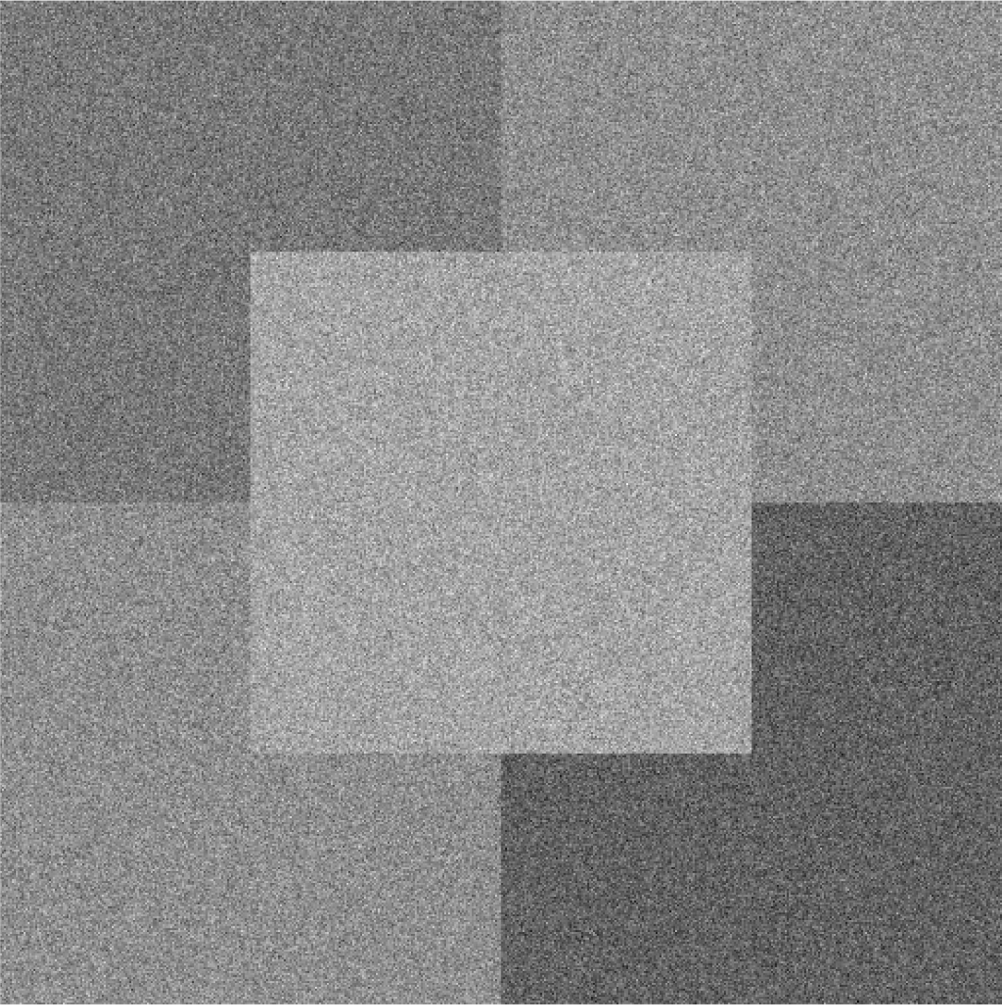
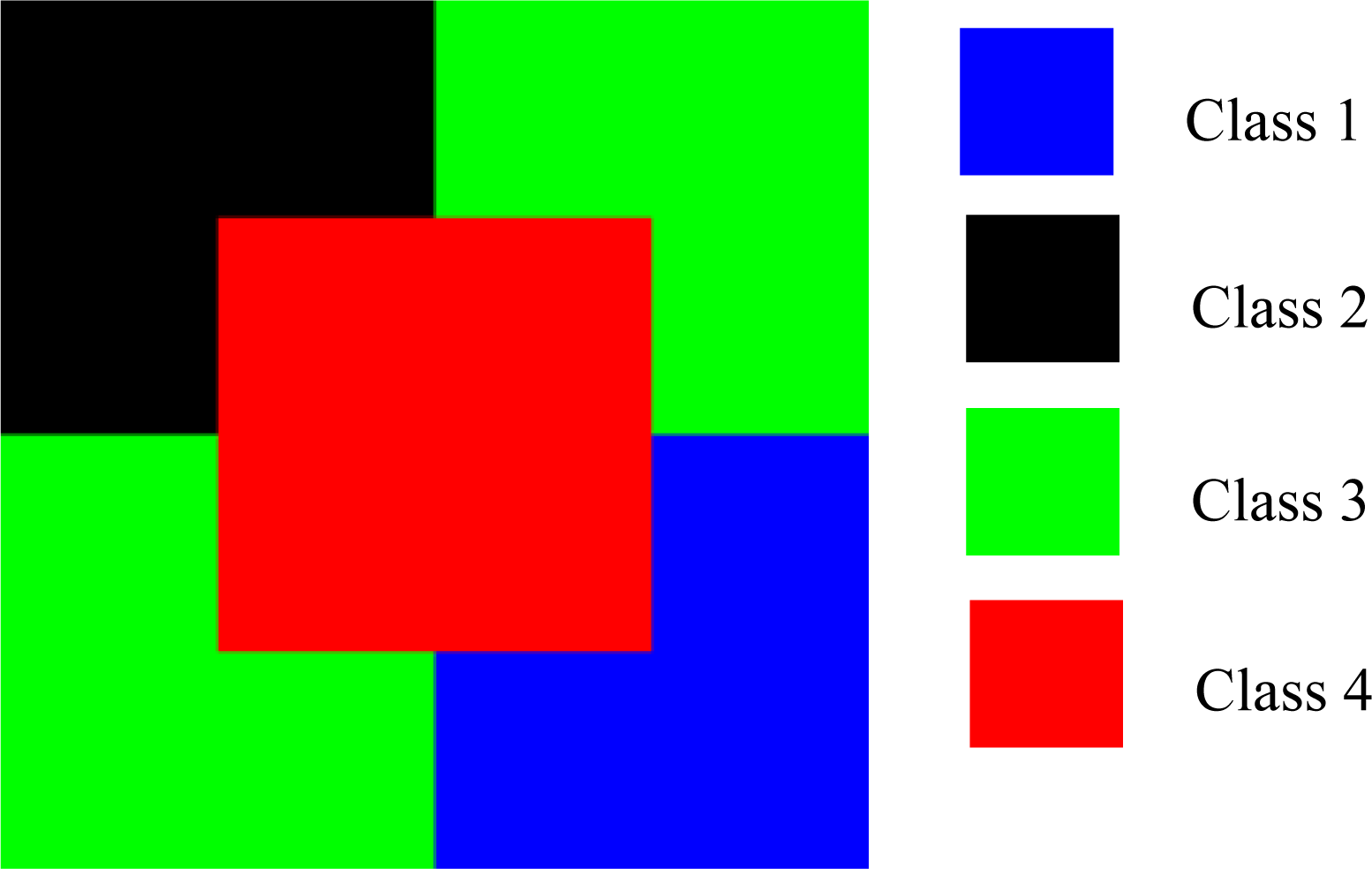
In the first experiment, we examined the performance of the proposed algorithm in terms of classification performance and registration accuracy by attempting to produce a land cover map from a set of four simulated images. All the simulated images were of an equal size of 512 × 512 pixels (Figure 3) and contained four land cover classes (Classes 1–4) with intensity values of zero, one, two and three for black, dark gray, light gray and white areas, respectively. Based on the noiseless image, the ground truth image in this example is provided in Figure 4 where the blue, black, green and red colors correspond to Classes 1–4, respectively. Next, all of the input images were added with the independent and identical Gaussian noise with a zero mean and standard deviation of σ = 1 to examine the performance of our proposed algorithm to image noise. Figure 5 shows an example of the input image for σ = 1. We perceived that the observed image appeared to be very noisy. We note here that all four noiseless simulated images are identical, and differ only once the noise has been added.

Since our algorithm performed both image registration and land cover mapping simultaneously, the performance of our algorithm could be evaluated in terms of how much the resulting LCM deviated from the reference LCM, and the estimation error between our calculated map parameters and the actual parameters that registered the LCM to the simulated images. If our algorithm performed perfect registration and land cover mapping, the resulting percentages of mis-classified pixels would be zero, and the registration error between the images and LCM would also be zero. In this example, the correct mapping parameters for all observed images were identical and equal to M_Perfect = [1,0,0,1,0,0] which correspond to unit scale, zero skew, and zero displacement. Next, since we wanted to examine the effects of the initial registration errors on the performance of our algorithm, we investigated different scenarios of initial registration errors by varying the initial mapping parameters between the observed images and LCM at different values of displacement, scale and skew parameters. In particular, we investigated three scenarios for only the displacement, only the scale and only the skew errors, respectively.

Table 1. Three scenarios for mapping parameter errors in Example 1.

	Image	Mapping Parameters
		m1	m2	m3	m4	m5	m6
Scenario I: Displacement error (δ)	1	1	0	0	1	0	0
	2	1	0	0	1	δ	0
	3	1	0	0	1	0	−δ
	4	1	0	0	1	−δ	δ
Scenario II: Scale error (ρ)	1	1	0	0	1	0	0
	2	1+ρ	0	0	1	0	0
	3	1	0	0	1+ρ	0	0
	4	1−ρ	0	0	1−ρ	0	0
Scenario III: Sheer error (η)	1	1	0	0	1	0	0
	2	1	η	0	1	0	0
	3	1	0	η	1	0	0
	4	1	−η	−η	1	0	0

shows the initial mapping parameters for all three scenarios. Here, δ, ρ and η are the initial displacement, scale, and skew parameter errors. Note that the initial mapping parameter errors for Image 1 for all scenarios were zero since we assumed that the first image is registered to the LCM as mentioned in Section 3.1.

Before investigating the performance of our proposed algorithm, we examined the effect of registration errors on the performance of image classification. This value can be viewed as the worst case scenario where the LCM is derived directly from the set of mis-registered images. Here, we employed the maximum likelihood classifier (MLC) [30] to the set of four remapped images, and the LCM was obtained from

$$x_s^{\mathit{MLC}}=\text{arg}\hspace{0.17em}\underset{x}{\text{min}}\left[\sum _{n=1}^4\left\{{\left({\mathit{z}}_{n,s}-{\mathit{\mu }}_{x_s,n}\right)}^T{\sum }_{x_s,n}^{-1}\left({\mathit{z}}_{n,s}-{\mathit{\mu }}_{x_s,n}\right)+\text{log}\left|{\sum }_{x_{s}n}\right|\right\}\right]$$

(37)

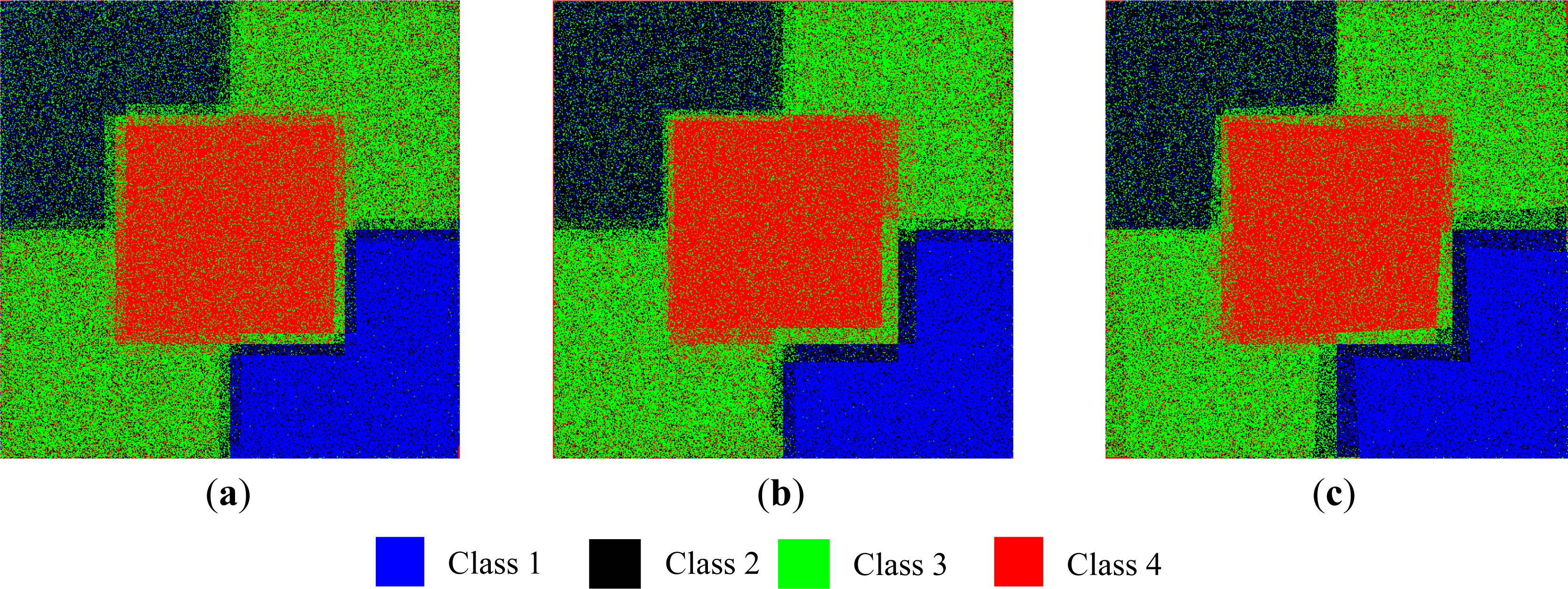
where the subscript n denotes the n-th remapped image. We note here that Equation (37) is the special case of the optimum LCM obtained from Equation (22) when β = 0. Figure 6a–c displays the resulting LCM for δ = 12 and σ = 1 for Scenario I, ρ = 0.05 and σ = 1 for Scenario II, and η = 0.05 and σ = 1 for Scenario III. We chose these values so that all scenarios yielded the averaged registration errors between 12 and 22 pixels or 2%–5% of the image size. The averaged percentages of misclassified pixels after a hundred independent runs are equal to 28.66%, 31.93% and 27.03%, for Scenarios I, II and III given above, respectively.

Next, the proposed algorithm was applied to the above datasets. The whole process was implemented using CUDA on NVIDIA Tesla M2090 with 1 GB memory. Here, we assigned $p^{\mathit{MF}}\left(x_s|\mathit{Y},{\mathit{M}}^0\right)=\frac{1}{4}$ as the most extreme case where no prior information was given. In different trials, the value of β was set to be 0.00, 0.25, 0.50, and 0.75 (see Equation (2)). Since our algorithm performed both image classification and registration, the termination criteria had to ensure the convergences in both the estimated posterior probability and mapping parameters. As a result, we defined

$$p_{\mathit{changes}}=\frac{1}{|𝒮|}\sum _{s\in 𝒮}\sum _{x_s\in \mathrm{\Lambda }}\left|p_s^{\mathit{MF}}\left(x_s|\mathit{Y},{\mathit{M}}^t\right)-p_s^{\mathit{MF}}\left(x_s|\mathit{Y},{\mathit{M}}^{t-1}\right)\right|$$

(38)

to measure changes in the posterior probabilities from two consecutive iterations. We also define

$$d_{\mathit{movement},n}=\frac{1}{|{𝒯}_n|}\sum _{\left(u_n,v_n\right)\in {𝒯}_n}\sqrt{{\left(x_n^t-x_n^{t-1}\right)}^2+{\left(y_n^t-y_n^{t-1}\right)}^2}$$

(39)

to characterize the movement of coordinates of the remapped image Z_n from two consecutive iterations where

$$\left[\begin{array}{l}{x}_n^t\hfill \\ y_n^t\hfill \end{array}\right]={\left[\begin{array}{ll}{m}_{1,n}^t\hfill & m_{2,n}^t\hfill \\ m_{3,n}^t\hfill & m_{4,n}^t\hfill \end{array}\right]}^{-1}\left[\begin{array}{l}{u}_n-m_{5,n}^t\hfill \\ v_n-m_{6,n}^t\hfill \end{array}\right]$$

(40)

Here, $m_{\text{i},\text{n}}^{\text{t}}$ denotes the mapping parameter m_i from the nth at the tth iteration. In this example, the algorithm terminates when p_changes is less than p_min = 10⁻⁵, and d_movement,n is less than 0.1 pixels for five consecutive iterations for n = 2,3,4. To create a benchmark for our proposed algorithm, we investigated two extreme cases where LCMs were derived directly from the unregistered image pairs and from a perfect registered image pair. The LCMs from these extreme cases were classified using our proposed algorithm by fixing M^t = M^*. For perfect registration, we had M^* = M_Perfect whereas, for unregistered image pairs, we set M^* equal to the values given in Table 1 for the respective scenarios. The first extreme case could be considered as the lower limit on the classification accuracy if we performed the land cover mapping without alignment of images first. The second case was an upper bound on the classification accuracy when we produced a map from a registered image pair. By setting up our experiment in this fashion, we could investigate how much improvement our algorithm could gain by integrating the registration and classification together, and how far the performance of our algorithm was from the upper limit where all uncertainties in registration were removed. To ensure the statistical significance of our experiment, all experiments were repeated ten times.

Table 2. Comparison of the averaged percentages of misclassified pixels (PMP) between two extreme cases and our proposed algorithm.

β	No Registration Error	No Registration Error Correction			Proposed Algorithm with Initial Registration Errors
		Scenario I with δ = 12	Scenario II with ρ = 0.05	Scenario III with η = 0.05	Scenario I with δ = 12	Scenario II with ρ = 0.05	Scenario III with η = 0.05
0.0	25.65%	28.66%	26.87%	27.05%	28.65%	26.07%	27.12%
0.25	0.43%	4.81%	5.96%	6.45%	0.45%	0.43%	0.43%
0.5	0.039%	4.24%	5.65%	6.21%	0.039%	0.041%	0.043%
0.75	0.021%	4.19%	5.56%	6.13%	0.024%	0.032%	0.026%

displays the averaged percentages of misclassified pixels (PMP) of the LCMs for different values of β and for Scenario I with δ = 12, Scenario II with ρ = 0.05 and Scenario III with η = 0.05 when σ = 1. Note here that, in this example, we employed the percentages of mis-classified pixels as the performance metric to evaluate the classification performance rather than the overall accuracy to highlight small differences in the classification performance between LCMs derived from image datasets without registration error and LCMs obtained from our proposed algorithm. From Table 2, it is clear that, from all scenarios, the PMPs derived from image datasets without registration errors corrections were always significantly poorer than those derived from registered image datasets. These results support our claims that it is important to consider a lack of alignments in performing image classification. We also observed that, for β = 0.25, 0.5 and 0.75, our proposed algorithm produced the LCM with an accuracy similar to those obtained from the image dataset without any registration errors. These results imply that our proposed algorithm attained the upper-bound accuracy with proper selection of the MRF parameter.

To ensure the statistical significance, we computed the pairwise t-statistics for unequal variance populations [29] of the PMPs obtained from LCMs derived from the proposed algorithm for various initial registration errors against those obtained from image dataset with no registration error, The resulting p-values [29] of the t-statistics are given in

Table 3. The p-values of the pairwise t-test with unequal variances of our proposed algorithm to the perfect registration cases. No registration error correction to the perfect registration cases.

β	No Registration Error	No registration Error Correction			Proposed Algorithm with Initial Registration Errors
		Scenario I with δ = 12	Scenario II with ρ = 0.05	Scenario III with η = 0.05	Scenario I with δ = 12	Scenario II with ρ = 0.05	Scenario III with η = 0.05
0.0	1	1.5 × 10−22	1.6 × 10−14	4.0 × 10−18	1.9 × 10−23	4.0 × 10−15	3.9 × 10−15
0.25	1	2.0 × 10−17	3.5 × 10−19	3.6 × 10−18	0.457	0.717	0.500
0.5	1	1.5 × 10−15	2.8 × 10−17	1.8 × 10−16	0.712	0.167	0.401
0.75	1	1.5 × 10−14	1.4 × 10−15	6.2 × 10−17	0.060	0.033	0.079

. The p-value represents the probability that there is no difference in PMPs. Hence, a smaller p-value implies that PMPs from two experiments are different. We also computed the t-statistics comparing LCMs obtained from the image dataset with and without registration errors. The resulting p-values of these t-statistics are also summarized in Table 3. It is clear from Table 3 that there are significant differences in term of PMPs from LCMs obtained from the image dataset with and without registration errors. Furthermore, the p-values also support our claim that for β = 0.25, 0.5 and 0.75, our proposed algorithm produced the LCM with an accuracy similar to those obtained from the image dataset without any registration errors. However at β = 0, our proposed algorithm performed significantly poorer than those of perfect registration. In fact, at β = 0, our proposed algorithm achieved roughly the same performance as in the situation where there is no registration error correction since, at β = 0, our proposed algorithm could not correctly estimate the map vectors. 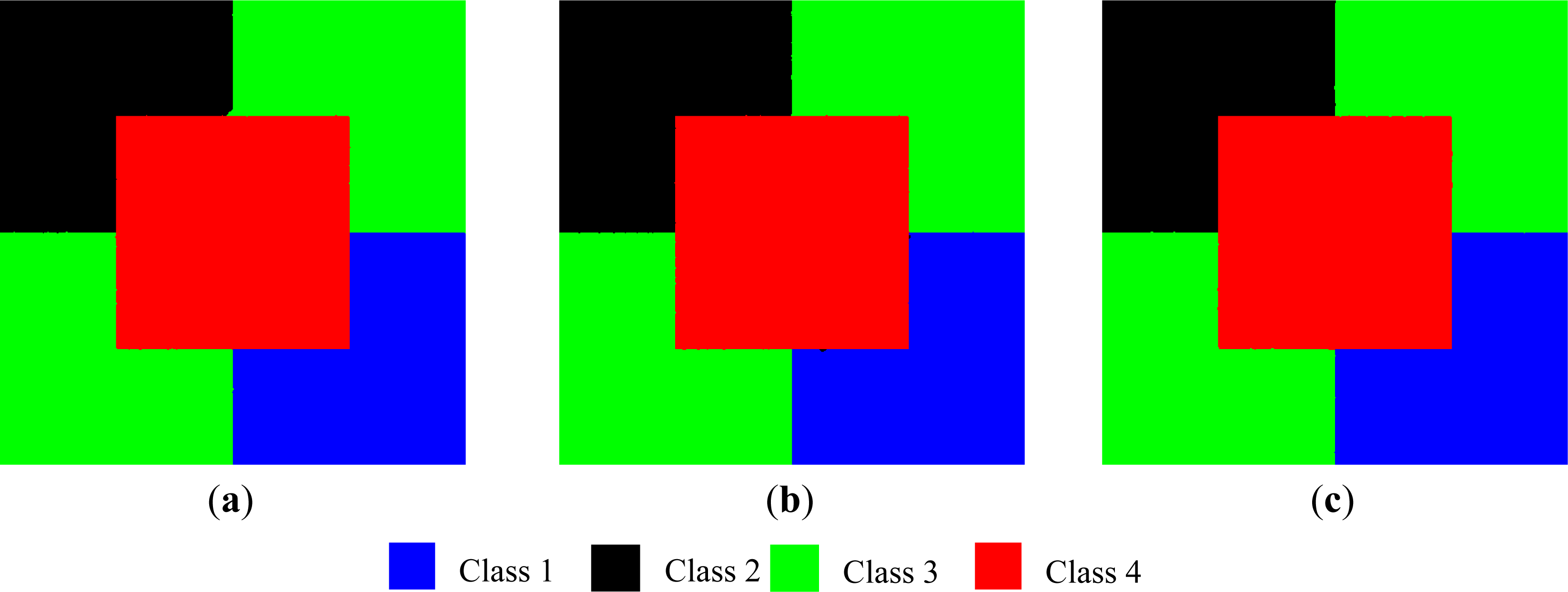Figure 7 shows examples of the resulting LCMs at β = 0.75 for all scenarios. We observed that all the LCMs appeared to be more connected than the MLC-based LCMs shown in Figure 6.

Since at β = 0.75, our proposed algorithm achieved the highest performance, we examined the effect of the initial registration errors to the performance of our algorithm by varying values of δ, ρ, and η for Scenarios I, II and III, respectively, for β = 0.75. Again, ten independent runs were performed to ensure the statistical significance and the results are given in

Table 4. The averaged percentages of mis-classified pixels as a function of the initial registration error for all Scenarios.

Scenario I		Scenario II		Scenario III
δ	PMP	ρ	PMP	η	PMP
0	0.019%	−0.05	0.035%	−0.05	0.036%
4	0.032%	−0.03	0.035%	−0.03	0.029%
8	0.029%	−0.01	0.022%	−0.01	0.043%
12	0.026%	0.01	0.030%	0.01	0.040%
		0.03	0.024%	0.03	0.036%
		0.05	0.032%	0.05	0.026%

. We observed that, for all scenarios, the PMPs were roughly the same. In other words, the initial registration errors had little effect on the performance of our algorithm. These results imply the robustness of our proposed algorithm to the initial mis-registration errors if the proper value of β is chosen.

Another key performance metric in this example is the residual registration errors after processing.

Table 5. The residual registration errors of our proposed algorithm for various scenarios and values of β.

Scenario			No Registration Error Correction	β = 0.0	β = 0.25	β = 0.50	β = 0.75
I (δ = 12)	Image 2	Mean	12	11.99	0.111	0.295	0.280
		STD	-	0.0015	0.259	0.139	0.100
	Image 3	Mean	12	11.99	0.031	0.192	0.312
		STD	-	0.0018	0.020	0.120	0.156
	Image 4	Mean	16.97	16.96	0.213	0.338	0.212
		STD	-	0.0017	0.566	0.088	0.136
II (ρ =0.05)	Image 2	Mean	14.06	13.56	0.028	0.281	0.327
		STD	-	0.072	0.010	0.130	0.113
	Image 3	Mean	14.06	13.49	0.020	0.353	0.312
		STD	-	0.032	0.080	0.102	0.106
	Image 4	Mean	21.97	20.97	0.253	0.245	0.315
		STD	-	0.095	0.636	0.120	0.082
III (η = 0.05)	Image 2	Mean	14.76	14.71	0.025	0.295	0.296
		STD	-	0.204	0.020	0.149	0.098
	Image 3	Mean	14.76	14.73	0.017	0.415	0.350
		STD	-	0.182	0.006	0.090	0.136
	Image 4	Mean	21.72	22.04	0.350	0.312	0.371
		STD	-	0.0325	0.983	0.155	0.088

displays the means and standard deviations of the root mean square errors (RMSEs) from ten independent runs between each of the simulated images and the reference LCM. The RMSE of the n-th image is computed from

$${\mathit{RMSE}}_n=\frac{1}{|{𝒯}_n|}\sum _{\left(u_n,v_n\right)\in {𝒯}_n}\sqrt{{\left(x_n^{gt}-x_n^{\mathit{est}}\right)}^2+{\left(y_n^{gt}-y_n^{\mathit{est}}\right)}^2}$$

(41)

where ( $x_n^{gt}$, $y_n^{gt}$) and ( $x_n^{\mathit{est}}$, $y_n^{\mathit{est}}$) are the ground truth and estimated coordinates. Here, the ground truth coordinates obtained by letting M_n = M_perfect. Clearly, for β = 0.25, 0.5, and 0.75, our algorithm can successfully register all images with the LCMs. However, at β = 0, our algorithm could not align these images with the LCM. The results in Table 5 emphasize the importance of parameter selection. Note here that the RMSE of Image 1 is not shown in Table 5 since it is assumed to be perfectly aligned (registration error is zero) with the LCM.

Next, we examined the effects of image noise on the registration accuracy by varying the noise variance σ² from −30 dB to 0 dB, and the resulting averaged RMSEs for β = 0.0 and 0.75 are given in

Table 6. The residual registration errors for various noise variances and β = 0.75.

Noise Variance (dB)	Average Root Mean Square Errors
	Scenario I, δ = 12			Scenario II, ρ= 0.05			Scenario III, η = 0.05
	Image 2	Image 3	Image 4	Image 2	Image 3	Image 4	Image 2	Image 3	Image 4
−30	0.007	0.011	0.009	0.006	0.010	0.019	0.012	0.019	0.013
−20	0.010	0.012	0.009	0.023	0.016	0.012	0.017	0.016	0.011
−10	0.036	0.035	0.037	0.028	0.018	0.029	0.028	0.030	0.022
0	0.244	0.280	0.185	0.119	0.138	0.071	0.078	0.053	0.200

and

Table 7. The residual registration errors for various noise variances and β = 0.

Noise Variance (dB)	Average Root Mean Square Errors
	Scenario I, δ = 12			Scenario II, ρ= 0.05			Scenario III, η = 0.05
	Image 2	Image 3	Image 4	Image 2	Image 3	Image 4	Image 2	Image 3	Image 4
−30	0.016	0.08	0.010	0.015	0.007	0.019	0.009	0.011	0.019
−20	0.017	0.012	0.014	0.015	0.018	0.015	0.010	0.015	0.017
−10	0.014	0.018	0.015	0.018	0.018	0.023	0.019	0.016	0.014
0	11.99	11.99	16.97	11.91	11.89	20.28	12.75	12.79	20.61

, respectively. We observed here that there were slight performance differences in term of the RMSEs for σ² of −30, −20 and −10 dB for both β = 0.00 and 0.75. However, for the noise variance equal to 0 dB, our algorithm could only correctly align Images 2–4 with the LCM at β = 0.75. This result emphasizes the importance of the MRF model to the convergence of our algorithm.

For the performance comparison, we compared the registration accuracy of our proposed algorithm for various scenarios and β = 0.75. with a traditional image-to-image registration technique. Here, we employed the mean square error criteria (MSEC) [8,34] since MSEC is suitable for registering images with the same modality and suffering from additive Gaussian noise. For the traditional image-to-image registration, we registered Images 2–4 with Image 1 since Image 1 was assumed to be aligned with the LCM. The averaged RMSEs from ten independent runs for various noise variances are shown in

Table 8. The residual registration errors using the minimum mean square error criteria for various noise variances.

Noise Variance (dB)	Image 2		Image 3		Image 4
	Mean	STD	Mean	STD	Mean	STD
−30	0.008	0.0029	0.007	0.0041	0.010	0.0054
−20	0.422	0.0040	0.425	0.0033	0.423	0.0049
−10	0.663	0.0037	0.665	0.0014	0.664	0.0017
0	0.875	0.516	1.637	1.441	1.352	0.9744

. Again, the particle swamp optimization algorithm with eighty particles was employed to ensure global optimality. As expected, the registration accuracy decreased as the noise variance increased. By comparing Tables 6 and 8, the RMSEs from our proposed algorithm seem to be lower (better) than those obtained from MSEC for noise variances equal to −20, −10 and 0 dBs, respectively.

Next, we again performed the pairwise t-test to determine whether there were significant differences in RMSEs obtained from our proposed algorithm and MSEC. The resulting p-values [29] are shown in

Table 9. The p-value from the pairwise t-test between the traditional registration method and our proposed algorithm for various scenarios at β = 0.75.

Noise Variance (dB)	Average Root Mean Square Errors
	Scenario I, δ = 12			Scenario II, ρ= 0.05			Scenario III, η = 0.05
	Image 2	Image 3	Image 4	Image 2	Image 3	Image 4	Image 2	Image 3	Image 4
−30	0.829	0.402	0.883	0.413	0.413	0.201	0.507	0.092	0.407
−20	1 × 10−18	4 × 10−14	2 × 10−21	1 × 10−13	1 × 10−13	3 × 10−15	2 × 10−13	2 × 10−13	5 × 10−17
−10	3 × 10−14	2 × 10−14	3 × 10−14	3 × 10−15	3 × 10−15	5 × 10−16	2 × 10−23	1 × 10−14	7 × 10−17
0	0.004	0.016	0.004	0.001	0.001	0.003	0.0010	0.007	0.004

. From the p-values, we can conclude that our proposed algorithm achieves significantly better registration accuracies than those obtained from MSEC for the noise variances of −20, −10 and 0 dBs. Note here that, for a noise variance equal to −30 dB, the registration errors from our proposed algorithm and the MSEC were roughly zero and, therefore there was no difference in terms of registration accuracy. Another key performance metric is the processing time. For noise variance equal to 0 dB, the total processing time for image-to-image registration was 170 s whereas our approach with β = 0.75 took 3,761, 6,063 and 4,620 s for Scenario I with δ = 12, Scenario II with, ρ= 0.05 and Scenario III with η = 0.05, respectively. However, the total processing times for our approach with β = 0.25 reduced 2,816, 1,039, and 989 s for Scenario I at δ = 12, Scenario II at ρ= 0.05 and Scenario III at η = 0.05, respectively. Clearly, our algorithm demanded more computation than the image-to-image registration based on MSEC. However, the computation time can be significantly reduced if a small value of β is chosen.

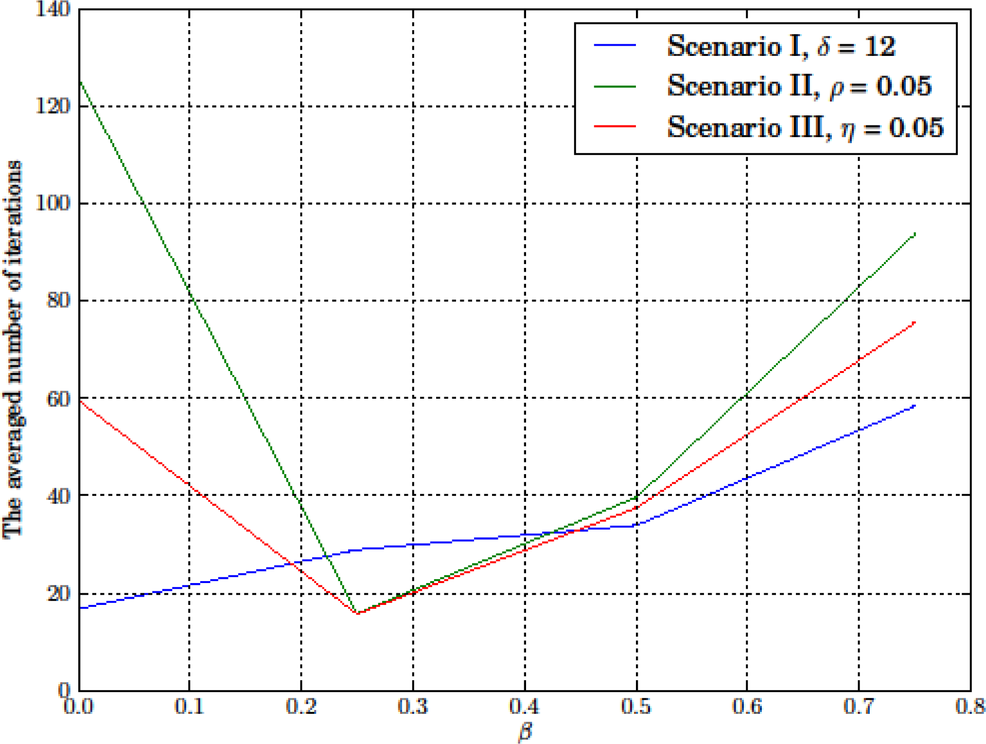
Figure 8 shows the averaged number of iterations that the algorithm required before the convergence criterion was satisfied for different scenarios and β. For β = 0.25, 0.5 and 0.75, more iterations were needed as the value of β increased. However, at β = 0, our algorithm terminated at the higher numbers of iterations than for β = 0.25 for Scenarios II and III whereas, for Scenario I, our algorithm terminated at the lower number of iterations. For Scenario I at β = 0, our algorithm quickly converged to the local optima since the resulting and initial registration errors shown in Table 5 were almost identical. The identical resulting and initial registration errors also suggested that this local optimum point was very close to the initial point. However, for Scenarios II and III at β = 0, the local optimum points might be further than in Scenario I, and the algorithm converged slowly due to the small changes in the mapping parameters from one iteration to another and since β = 0, these small changes in the mapping parameters had a significant influence on the posterior probability.

5.2. Experiment 2

A QuickBird dataset consisting of one multispectral image (MI) of size 150 × 300 pixels and one panchromatic image (PAN) of size 600 × 1,200 pixels was used in this experiment (Figure 9). The MI and PAN have resolutions of 2.4 and 0.6 m, respectively. Both images captured a part of Kasetsart University in Bangkok, Thailand, covering around 0.2592 km², on 10 July 2008. Through visual interpretation, we classified the area into five classes, namely, water, shadow, vegetation, and impervious type 1 and impervious type 2. The ground truth image is shown in Figure 10 where the blue, black, green, red and white colors correspond to water, shadow, vegetation, impervious type 1 and impervious type 2, respectively. In this case, the impervious was divided into two types due to different roof and pavement colors in the scene. By using both PAN and MI images, we randomly selected 1,000 samples for each land cover class.

In Experiment 2, we focused on the robustness of the proposed algorithm with respect to different degrees of the initial displacement, scale and rotation errors. In fact, there were six displacement errors in the x-direction and y-direction, four scale errors and six rotational errors in this experiment. The termination criteria used in this example were similar to those in Example 1, i.e., our algorithm was terminated if p_changes (see Equation (38)) was less than 10⁻⁵ and d_movement,MI (see Equation (39)) was less than 0.1 pixels for five consecutive iterations. Before examining the robustness of our algorithm, we determined the benchmark performance of the MRF-based land cover mapping when MI and PAN were perfectly registered. The resulting LCMs are shown in Figure 11. Again, as we progressed to greater values of β, more connected LCMs are obtained. The overall accuracy graph shown in Figure 12 agrees with the visual inspection that the classification performance increased as the values of β increased. In this example, we employed the overall accuracy rather than the percentages of mis-classified pixels used in Example 1 since overall accuracy is a more widely used performance metric in remote sensing image classification.

Since the PAN had a higher resolution, we assumed that it was aligned with the LCM, and we only needed to find the map parameters of the MI. Here, the PAN has a higher resolution than the multispectral image by the factor of four, and both MI and PAN were obtained from the same satellite. The optimal map parameter vector relating the two images was therefore be equal to

$$M^{\mathit{opt}}=[0.25,0,0,0.25,0,0].$$

To investigate the robustness of our algorithm to displacement, scale and rotation errors, we introduced the registration errors in displacement in the x-direction, displacement in the y-direction, scale and rotation into the MI and PAN pair. If we introduced the displacements into the image pair, the initial map parameter was set to be equal to

$${\text{M}}^0=[0.25,0,0,0.25,\mathrm{\Delta }\text{x},0]$$

and

$${\text{M}}^0=[0.25,0,0,0.25,0,\mathrm{\Delta }y],$$

for displacement errors in the x- and y-direction, respectively. Here, the values of Δx and Δy was set as −5, −3, −1, 1, 3, and 5. For the scale and rotation errors, we assumed that both images were aligned at mid points, i.e., the pixel (75,150) of MI was at the pixel (300,600) of PAN. Next, we applied the initial scale errors, Δs, of −5%, −2.5%, 0%, 2.5% and 5% when comparing the PAN image with the multispectral image. Here, the scale errors of −5%, −2.5%, 0%, 2.5% and 5% corresponded to the initial scales of PAN to MI of 3.8, 3.9, 4.0, 4.1 and 4.2, respectively. For rotation errors, we rotated the MI by Δθ degrees in a counter clockwise direction. Here, the initial rotation errors Δθ were set as −3°, −2°, −1°, 1°, 2° and 3°. The initial RMSE_MI (see Equation (41)) for all cases are given in

Table 10. The initial RMSE_MI in meters (pixels in LCM) for various cases in Example 2.

Error in x-Direction		Error in y-Direction		Error in Scale		Error in Rotation
Δx	RMSEMI	Δy	RMSEMI	Δs	RMSEMI	Δθ	RMSEMI
−5	12 (20)	−5	12 (20)	−5%	21.3 (36)	−3	11.12 (19)
−3	7.2 (12)	−3	7.2 (12)	−2.5%	10.7 (18)	−2	7.45 (12)
−1	2.4 (4)	−1	2.4 (4)	0%	0.0 (0)	−1	3.72 (6.2)
1	2.4 (4)	1	2.4 (4)	2.5%	10.7 (18)	1	3.72 (6.2)
3	7.2 (12)	3	7.2 (12)	5%	21.3 (36)	2	7.45 (12)
5	12 (20)	5	12 (20)			3	11.12 (19)

. Again, if our algorithm performed perfectly, the estimated map parameter would converge back to M^opt. In other words, we would eventually end up with M^t = M^opt. Once the correct map parameter vector was obtained, the classification accuracies of the LCMs were expected to be equal to those of the perfect registration cases (Figure 11a–d). In this example, we again assigned $p^{\mathit{MF}}\left(x_s|\mathit{Y},{\mathit{M}}^0\right)=\frac{1}{5}$, the most extreme case where no prior information was given.

The overall accuracies as a function of Δx, Δy, Δs, and Δθ are shown in Figure 13a–d, respectively. From almost all scenarios, the overall accuracies increased as the value of β increased since the MRF model promoted more connected land cover maps, and, therefore, removed the isolated misclassified pixels. However, for Δx = 5 and Δy = 5, the overall accuracies of our algorithms decreased as β increased. These performance degradations were mainly due to the fact that our algorithm terminated on one of the local optima since the EM algorithm employed in our work cannot guarantee the global optimum solution. The evidence can be seen Figure 14a–b. In Figure 14a, we observed that, for almost all of the initial values of Δx, the number of iterations increased as the value β increased. However, for Δx = 5.0, our algorithm terminated at only 75, 109 and 129 iterations for β = 0.25, 0.5 and 0.75 whereas, for β = 0.0, our algorithm terminated after 180 iterations. Similarly, we observed the same phenomena in Figure 14b for Δy = 5.0 where the algorithm terminated at a lower number of iterations for β = 0.75 than for β = 0.0, 0.25 and 0.50. This result showed the effects of the initial registration errors on the convergence of our algorithm. In most practical situations, such large initial registration errors are unlikely to occur since most remote sensing images are embedded with coordinate information from a producer.

Similar to the previous example, we also compared the performance of our proposed algorithm (PA) with two extreme cases where images were perfectly registered (PR) and there was no registration error correction (NC). The results are provided in

Table 11. Overall accuracies for different values of β in two extreme cases and our proposed algorithm for different initial displacement error in the x-direction Δx where PA and NC denote the cases of the proposed algorithm and no registration error correction, respectively.

β	PR	Δx = −5.0		Δx = −3.0		Δx = −1.0		Δx = 1.0		Δx = 3.0		Δx = 5.0
		PA	NC	PA	NC	PA	NC	PA	NC	PA	NC	PA	NC
0.0	67.5	67.7	57.6	67.8	62.2	67.7	66.9	67.8	66.7	67.7	61.8	67.8	57.0
0.25	69.4	70.0	58.8	69.8	63.7	69.8	68.6	69.9	68.3	70.0	63.4	59.3	58.4
0.5	70.3	71.8	59.7	71.4	64.6	70.6	69.6	70.9	69.2	71.5	64.4	60.2	59.2
0.75	71.1	72.8	60.2	72.2	65.2	71.5	70.3	71.8	70.0	72.7	65.0	60.4	59.9

Table 12. Overall accuracies for different values of β in two extreme cases and our proposed algorithm for different initial displacement error in the y-direction Δy where PA and NC denote the cases of the proposed algorithm and no registration error correction, respectively.

β	PR	Δy = −5.0		Δy = −3.0		Δy = −1.0		Δy = 1.0		Δy = 3.0		Δy = 5.0
		PA	NC	PA	NC	PA	NC	PA	NC	PA	NC	PA	NC
0.0	67.5	67.7	57.6	67.7	62.2	67.7	66.9	67.7	66.7	67.7	61.8	67.8	57.0
0.25	69.4	69.9	58.8	69.9	63.7	69.8	68.6	70.1	68.3	70.1	63.4	70.3	58.4
0.5	70.3	71.6	59.7	71.2	64.6	70.5	69.6	71.8	69.2	71.8	64.4	68.6	59.2
0.75	71.1	72.5	60.1	71.9	65.2	71.2	70.3	73.4	70.0	73.4	64.9	62.9	59.9

Table 13. Overall accuracies for different values of β in two extreme cases and our proposed algorithm for different initial scale error Δs where PA and NC denote the cases of the proposed algorithm and no registration error correction, respectively.

β	PR	Δs = −5%		Δs = −2.5%		Δs = 0%		Δs = 2.5%		Δs = 5%
		PA	NC	PA	NC	PA	NC	PA	NC	PA	NC
0.0	67.5	67.8	52.7	67.7	61.0	67.7	67.5	67.8	64.9	67.8	57.8
0.25	69.4	69.6	53.4	69.5	62.4	70.0	69.4	70.3	66.1	70.2	58.9
0.5	70.3	71.1	54.2	70.6	63.3	71.0	70.3	71.6	67.0	72.1	59.7
0.75	71.1	72.1	54.7	71.5	64.2	71.1	71.1	72.7	67.6	73.4	60.1

and

Table 14. Overall accuracies for different values of β in two extreme cases and our proposed algorithm for different rotation error Δθ where PA and NC denote the cases of the proposed algorithm and no registration error correction, respectively.

β	PR Registration	Δθ = −3°		Δθ = −2°		Δθ = −1°		Δθ = 1°		Δθ = 2°		Δθ = 3°
		PA	NC	PA	NC	PA	NC	PA	NC	PA	NC	PA	NC
0.0	67.5	67.6	57.3	67.6	60.8	67.6	65.3	67.7	64.8	67.7	59.8	67.8	55.5
0.25	69.4	69.9	58.5	69.8	62.2	69.7	66.9	69.9	66.5	69.7	61.1	69.8	56.6
0.5	70.3	71.6	59.3	71.4	63.0	71.0	67.8	71.1	67.4	71.4	62.0	71.5	57.4
0.75	71.1	73.0	59.7	72.3	63.6	71.9	68.4	71.9	68.1	72.5	62.6	72.9	58.0

. From this comparison, we observed that if our algorithm converged to the global optimum solutions, the resulting overall accuracies from our proposed algorithm were similar to those of the perfect registration cases, and significant improvements were obtained from the cases where there was no registration error correction. The maximum performance improvements from no registration error correction for each cases were 12.6% for Δx = −5 and β = 0.75, 12.4% for Δy = −5 and β = 0.75, 17.4% for Δs = −5% and β = 0.75, and 14.9% for Δθ = 3° and β = 0.75, respectively. We observed that the maximum improvements were achieved at β = 0.75. This observation suggested that a higher performance gain could be obtained by increasing the value of β.

Next, we also noticed that our proposed algorithm could sometimes achieve even higher accuracies than those of the perfect registration cases. This was due to the fact that our algorithm required more iterations than the scenarios where the image pair was perfectly registered since our algorithm terminated if both the estimated map parameters and the resulting LCM converged whereas, in the perfect registration case, the process terminated if only the resulting LCM converged. Hence, our algorithm might terminate at lower percentages of changes in the LCM, and lead to more accurate LCM which, in turn, resulted in higher precision.

Another key performance metric of our algorithm was the resulting registration errors. Figure 15a–d show the residual registration errors in terms of RMSE (in meters) between the MS image and the LCM for different initial registration errors. We observed that, if our algorithm converged to the global optimum solution, it could successfully reduce the registration error down to around 1.8 m in the LCM (or equivalently, 0.75 pixels on the MS image and 3 pixels on the PAN image and LCM). These results imply that our algorithm can align images together to the accuracy less than those of the lowest resolution (which was the MS image in our case). For each initial registration error cases, the minimum RMSEs of 1.718 (2.86 pixels in the LCM) m for Δx = 1.0, 1.672 (2.79 pixels in the LCM) m for Δy = 1.0, 1.730 (2.88 pixels in the LCM) m for Δs = 0%, and 1.704 (2.84 pixels in the LCM) m for Δθ = −1° occurried at β = 0.75. These results suggest that, if our algorithm converges, the larger value of β increases the accuracy of registration as well as the classification. However, for the cases of Δx = 5.0 and Δy =5.0, our algorithm could not register the MS image to the LCM since our algorithm was stuck in one of the local optima. The residual registration errors for Δx = 5.0 were 1.896 (3.16), 10.96 (18.3), 11.14 (18.6), and 11.41 (19.0) m (pixels in the LCM), and for Δy = 5.0 were 1.827 (3.05), 1.834 (3.06), 3.133 (5.22) and 11.57 (19.3) m (pixels in the LCM) for β = 0.0, 0.25, 0.50, and 0.75, respectively. Here, the initial displacement error corresponded to the RMSE of 20 pixels in the LCM. Such a large initial RMSE is only found when remote sensing images have significant differences in spatial resolutions. LCMs derived from remote sensing image datasets with such a large scale difference are often unreliable and seldom found in practice.

For performance comparison, we applied the normalized cross correlation method [34] to register the PAN and MS images together, and the resulting RMSE was equal to 1.836 m or 3.06 pixels in the LCM. From Figures 15a–d, we found that, with proper parameter selections and the initial registration errors, our proposed algorithm can achieve a higher registration accuracy than those from the normalized cross correlation method. For example, our algorithm obtained registration errors of 1.718 (2.86 pixels) m for β = 0.75 and Δx = 1, 1.671 (2.79 pixels) m for β = 0.75 and Δy = 1, or 1.702 (2.84 pixels) m for β = 0.75 and Δθ = −1°.

Based on the experimental results shown in Figure 13a–d and Figure 15a–d, we conclude that our proposed algorithm achieves higher classification and registration accuracy as the value of β increases, if the initial registration error is sufficiently small (e.g., for Δx = ±1, Δy = 1, Δs = 0, and Δθ = ±1). However, if the initial registration error increases beyond a certain point, our algorithm is more likely to terminate in one of the local optima as the value of β increases. Hence, if images have a high degree of misalignment, a low value of β should be chosen. However, if images are pre-aligned with any simple registration process, a higher value of β is preferable. In fact, most available remote sensing images nowadays are pre-registered to a map coordinate system with a limited degree of accuracy. As a result, the misalignment in image datasets should be limited, and in the practical use of our proposed algorithm, we recommended a high value of β.

6. Conclusion

In this paper, we propose a joint image registration and land cover mapping algorithm based on a Markov random field model. By combining image registration and classification into a single process, the classification performance of our proposed algorithm is not affected by the registration errors in image datasets, whereas the performance of traditional image classification algorithms can be significantly degraded due to registration errors.

In our work, the algorithm assumes that observed remote sensing images are derived from a hidden land cover map and captured with an unknown misalignment. Two adjacent pixels of the land cover map are more likely to belong to the same land cover class than different classes. By integrating this fact into the model, a large number of misclassified pixels, which often appear as isolated pixels, are removed from the resulting land cover map. Since the map parameter vector relating the different images is unknown, we employ the expectation-maximization procedure to simultaneously estimate the map parameters and use mean field theory to approximate the posterior probability.

We performed an experimental study using one simulated dataset, and one real remote sensing dataset of 2.4 m QUICKBIRD multispectral and 0.6 m QUICKBIRD panchromatic images. Our results show that, for the first data set, our algorithm can successfully classify image pairs and align them in different initial registration errors with proper selection of the Markov random field parameter. In fact, if the Markov random field parameter is chosen properly, our algorithm can classify mis-registered image pairs with a similar accuracy to the situation where images are perfectly aligned. For the real remote sensing dataset, we focused the investigation on the robustness of our algorithm to the initial alignment of image pairs. The study revealed that our algorithm is less sensitive to the initial alignment when the value of the Markov random field parameter is small since the expectation-maximization algorithm tends to converge faster.

One major limitation of our proposed algorithm is that the expectation-maximization algorithm employed in our algorithm tends to be trapped in local optima if the initial misalignment is large. Hence, in the future, we plan to investigate how to incorporate a different variation of the expectation-maximization algorithm that can escape from local optima in order to make our algorithm more robust. Another limitation of our algorithm is its sensitivity to the Markov random field parameter selection. To address this problem, we plan to investigate how to automatically tune the Markov random field parameter so that the joint image registration and classification can be performed without the initial Markov random field parameter section.

References

1. Lombardo, P.; Oliver, C.J.; Pellizzeri, T.M.; Meloni, M. A new maximum-likelihood joint segmentation technique for multitemporal sar and multiband optical images. IEEE Trans. Geosci. Remote Sens 2003, 41, 2500–2518. [Google Scholar]
2. Skriver, H.; Mattia, F.; Satalino, D.; Balenzano, A.; Pauwells, V.R.N.; Verhoest, N.E.C.; Davison, M. Crop classification using short-revisit multitemporal SAR data. IEEE J. Sel. Top. Appl. Earth Obs. Remote Sens 2011, 4, 423–431. [Google Scholar]
3. Baghdadi, N.; Todoroff, P.; Hjj, M.E.; Begue, A. Potential of SAR sensors TerraSAR-X, ASAR/ENVISAT and PALSAR/ALOS for monitoring sugarcane crops on Reunion Island. Remote Sens. Environ 2009, 113, 1724–1738. [Google Scholar]
4. Meroni, M.; Marinho, E.; Sghaier, N.; Verstrate, M.M.; Leo, O. Remote sensing based yield estimation in a stochastic framework—case study of durum wheat in Tunisia. Remote Sens 2013, 5, 539–557. [Google Scholar]
5. Khedam, R.; Belhadj-aissa, A. A General Multisource Contextual Classification Model of Remotely Sensed Imagery Based on MRF. Proceedings of Remote Sensing and Data Fusion over Urban Areas, IEEE/ISPRS Joint Workshop 2001,. Rome, Italy, 8–9 November 2001; pp. 231–235.
6. Thoonen, G.; Mahmood, Z.; Peeters, S.; Scheunders, P. Multisource classification of color and hyperspectral images using color attribute profiles and composite decision fusion. IEEE J. Sel. Top. Appl. Earth Obs. Remote Sens 2012, 5, 510–521. [Google Scholar]
7. Camps-Valls, G.; Gomez-Chova, L.; Munoz-Mari, J.; Rojo-Alvarez, J.L.; Martinez-Ramon, M. Kernel-Based framework for multitemporal and multisource remote sensing data classification and change detection. IEEE Trans. Geosci. Remote Sens 2008, 1822–1835. [Google Scholar]
8. Hasan, M.; Pickering, M.R.; Jia, X. Robust automatic registration of multi-modal satellite images using CCRE with partial volume interpolation. IEEE Trans. Geosci. Remote Sens 2012, 50, 4050–4061. [Google Scholar]
9. Brook, A.; Ben-Dor, E. Automatic registration of airborne and spaceborne images by topology map matching with surf processor algorithm. Remote Sens 2011, 3, 65–82. [Google Scholar]
10. Mahapatra, D.; Sun, Y. Integrating segmentation information for improved MRF-based elastic image registration. IEEE Trans. Image Process 2012, 21, 170–183. [Google Scholar]
11. Chen, S.; Guo, Q.; Leung, H.; Bosse, E. A maximum likelihood approach to joint image registration and fusion. IEEE Trans. Image Process 2011, 20, 1363–1372. [Google Scholar]
12. Winkle, G. Image Analysis Random Fields and Dynamic Monte Carlo Methods; Springer-Verlag: New York, NY, USA, 1995. [Google Scholar]
13. Bremaud, P. Markov Chains Gibbs Field, Monte Carlo Simulation, and Queues; Springer-Verlag: New York, NY, USA, 1999. [Google Scholar]
14. Geman, S.; Geman, D. Stochastic relaxation, gibbs distributions, and the bayesian restoration of images. IEEE Trans. Pattern Anal. Mach. Intell 1984, 6, 721–741. [Google Scholar]
15. Solberg, A.H.S.; Taxt, T.; Jain, A.K. A Markov random field model for classification of multisource satellite imagery. IEEE Trans. Geosci. Remote Sens 1996, 34, 100–113. [Google Scholar]
16. Kasetkasem, T.; Varshney, P.K. An image change detection algorithm based on Markov random field models. IEEE Trans. Geosci. Remote Sens 2002, 40, 1815–1823. [Google Scholar]
17. Bruzzone, L.; Prieto, D.F. Automatic analysis of the difference image for unsupervised change detection. IEEE Trans. Geosci. Remote Sens 2002, 38, 1171–1182. [Google Scholar]
18. Xie, H.; Pierce, L.E.; Ulaby, F.T. SAR speckle reduction using wavelet denoising and Markov random field modeling. IEEE Trans. Geosci. Remote Sens 2002, 40, 2196–2212. [Google Scholar]
19. Peng, Y.; Chen, J.; Xu, X.; Pu, F. SAR images statistical modeling and classification based on the mixture of alpha-stable distributions. Remote Sens 2013, 5, 2145–2163. [Google Scholar]
20. Xu, M.; Chen, H.; Varshney, P. An image fusion approach based on Markov random fields. IEEE Trans. Geosci. Remote Sens 2011, 49, 5116–5127. [Google Scholar]
21. Wang, L.; Wang, Q. Subpixel mapping using Markov random field with multiple spectral constraints from subpixel shifted remote sensing images. IEEE Trans. Geosci. Remote Lett 2013, 10, 598–602. [Google Scholar]
22. Kasetkasem, T.; Arora, M.; Varshney, P.K. Super-resolution land cover mapping using a Markov random field based approach. Remote Sens. Environ 2005, 96, 302–314. [Google Scholar]
23. Moser, G.; Serpico, S.B.; Bennediktsson, J.A. Land cover mapping by Markov Modeling of spatial-contextual information in very high-resolution remote sensing images. Proc. IEEE 2013, 101, 631–651. [Google Scholar]
24. Dempster, A.P.; Laird, N.M.; Rubin, D.B. Maximum likelihood from incomplete data via the EM algorithm. J. R. Soc. Stat. Ser. B 1997, 39, 1–38. [Google Scholar]
25. Celeux, G.; Forbes, F.; Peyrard, N. EM procedures using mean field-like approximations for Markov model-based image segmentation. Pattern Recognit 2003, 36, 131–144. [Google Scholar]
26. Tanaka, T. Mean field theory of boltzmann machine learning. Phys. Rev. E 1998, 58, 2302–2310. [Google Scholar]
27. Tanaka, T. A Theory of Mean Field Approximation. Proceedings of 12th Annual Conference on Neural Information Processing Systems (NIPS’98), Denver, CO, USA, 30 November–5 December 1998.
28. Zhang, J. The mean field theory in EM procedures for Markov random fields. IEEE Trans. Signal Process 1992, 40, 2570–2583. [Google Scholar]
29. Bickel, P.J.; Doksum, K.A. Mathematical Statistics; Prentice Hall: Englewood Cliffs, NJ, USA, 1977. [Google Scholar]
30. Van Trees, H.L. Detection, Estimation, and Modulation Theory; Wiley: New York, NY, USA, 1968. [Google Scholar]
31. Varshney, P.K. Distributed Detection and Data Fusion; Springer: New York, NY, USA, 1997. [Google Scholar]
32. Kennedy, J.; Eberhart, R. Particle Swarm Optimization. Proceedings of IEEE International Conference on Neural Networks IV, Perth, WA, Australia, 27 November–1 December 1995; pp. 1942–1948.
33. Trelea, I.C. The particle swarm optimization algorithm: Convergence analysis and parameter selection. Image Process. Lett 2003, 85, 317–325. [Google Scholar]
34. Zitova, B.; Flusser, J. Image registration: A survey. Image Comput 2003, 21, 977–1000. [Google Scholar]
Figure 1. Clique types for (a) four-neighborhood; (b) eight-neighborhood.
Remotesensing 05 05089f1
Figure 2. Block diagram of the modified expectation maximization (EM) algorithm.
Remotesensing 05 05089f2
Figure 3. Noiseless Simulated Image in Example 1.
Remotesensing 05 05089f3
Figure 4. The ground data of Example 1.
Remotesensing 05 05089f4
Figure 5. An example of the noisy input image at σ = 1 in Example 1.
Remotesensing 05 05089f5
Figure 6. Examples of the maximum likelihood classifier (MLC)-based land cover maps (LCMs) for (a) Scenario I with δ = 12 and σ = 1; (b) Scenario II with ρ = 0.05 and σ = 1; and (c) Scenario III with η = 0.05 and σ = 1.
Remotesensing 05 05089f6
Figure 7. Examples of the resulting LCMs from our proposed algorithm (a) Scenario I with δ = 12 and σ = 1; (b) Scenario II with ρ = 0.05 and σ = 1; and (c) Scenario III with η = 0.05 and σ = 1.
Remotesensing 05 05089f7
Figure 8. The averaged number of iterations required before the termination criteria were satisfied for different scenarios in Example 1.
Remotesensing 05 05089f8
Figure 9. QUICKBIRD dataset of a part of Kasetsart University (a) False color composite multispectral image (MI); and (b) panchromatic image (PAN).
Remotesensing 05 05089f9
Figure 10. Ground truth image for Example 2 (green, blue, black, red and white colors for vegetation, water, shadow, impervious type 1 and impervious type 2, respectively).
Remotesensing 05 05089f10
Figure 11. LCMs for the perfect registration case for (a) β = 0; (b) β = 0.25; (c) β = 0.50; and (d) β = 0.75.
Remotesensing 05 05089f11aRemotesensing 05 05089f11b
Figure 12. Overall accuracies for different values of β when MI and PAN are perfectly aligned.
Remotesensing 05 05089f12
Figure 13. The effect of initial registration errors to the overall accuracies for (a) in the x-direction; (b) in the y-direction; (c) in the scale; and (d) in the rotation.
Remotesensing 05 05089f13
Figure 14. The effect of the initial registration errors to the number of iterations (a) in the x-direction; (b) in the y-direction; (c) in the scale; and (d) in the rotation.
Remotesensing 05 05089f14
Figure 15. The effect of the initial registration errors on the residual registration error of our proposed algorithm in Example 2.
Remotesensing 05 05089f15