An Enhanced Spatial and Temporal Data Fusion Model for Fusing Landsat and MODIS Surface Reflectance to Generate High Temporal Landsat-Like Data

Abstract

Remotely sensed data, with high spatial and temporal resolutions, can hardly be provided by only one sensor due to the tradeoff in sensor designs that balance spatial resolutions and temporal coverage. However, they are urgently needed for improving the ability of monitoring rapid landscape changes at fine scales (e.g., 30 m). One approach to acquire them is by fusing observations from sensors with different characteristics (e.g., Enhanced Thematic Mapper Plus (ETM+) and Moderate Resolution Imaging Spectroradiometer (MODIS)). The existing data fusion algorithms, such as the Spatial and Temporal Data Fusion Model (STDFM), have achieved some significant progress in this field. This paper puts forward an Enhanced Spatial and Temporal Data Fusion Model (ESTDFM) based on the STDFM algorithm, by introducing a patch-based ISODATA classification method, the sliding window technology, and the temporal-weight concept. Time-series ETM+ and MODIS surface reflectance are used as test data for comparing the two algorithms. Results show that the prediction ability of the ESTDFM algorithm has been significantly improved, and is even more satisfactory in the near-infrared band (the contrasting average absolute difference [AAD]: 0.0167 vs. 0.0265). The enhanced algorithm will support subsequent research on monitoring land surface dynamic changes at finer scales.

1. Introduction

Remotely sensed data, with high spatial resolution (HSR) and high temporal resolution (HTR), are very significant for monitoring rapid land surface changes (e.g., intraseasonal ecosystem variations) at fine scales (e.g., 30 m). However, the tradeoff in sensor designs, which balance spatial resolution and temporal coverage, make it difficult to acquire the data with “both high” characteristics [1]. For instance, the HTR data provided by some sensors (e.g., NOAA Advanced Very High Resolution Radiometer (AVHRR), Terra/Aqua Moderate Resolution Imaging Spectroradiometer (MODIS)) can be used in research at regional or global scales [2–4], but cannot reach the requirements of studies at local scales well, due to their low spatial resolutions (LSR) (250 m∼1,000 m). On the contrary, the HSR data acquired by other sensors (e.g., Landsat Thematic Mapper (TM) or Enhanced Thematic Mapper Plus (ETM+), SPOT High Resolution Visible (HRV)) can be applied for land-use/cover mapping and dynamic change detection at fine spatial resolutions [5–7], but can rarely be used to capture the changes in crop phenology and crop growth due to their low temporal resolutions (LTR) (e.g., Landsat TM: 16 d; SPOT HRV: 26 d) and frequent cloud contamination.

Blending observations from multiple sensors with different advantages or characteristics (e.g., ETM+ and MODIS) is considered as a feasible and less expensive way to solve the “spatial-temporal contradiction” [8–10]. Several fusion algorithms have developed from this idea in recent years. Gao et al. [11] brought forward the Spatial and Temporal Adaptive Reflectance Fusion Model (STARFM) for fusing Landsat and MODIS surface reflectance data to produce a synthetic “daily” surface reflectance product at the ETM+ spatial resolution. Some studies [11,12] pointed out that the algorithm could, generally, fuse those data to generate the predicted images in good agreement with actual observations. However, it would lead to some errors, to some degree, in the following cases: (1) no transient change information of ground objects is recorded in the base Landsat images; and (2) no homogeneous LSR pixels appear in the sliding window. Regarding case (1), Hilker et al. [9] added the day of disturbed (DoD) information, extracted from the time-series MODIS images, to the judgment condition to select the base image pair. The rule is that the first Landsat and MODIS image pair is selected if the prediction date lies before the DoD (T₀ < DoD); otherwise, the last one is selected (T₀ ≥ DoD). Regarding the case (2), Zhu et al. [13] introduced the conversion factor (v) related to endmembers, and made the assumption that the endmember reflectance experiences linear change in a short period to “separate” more accurate reflectance variations of different endmembers from LSR pixels. They also calculated the correlation coefficient (R) between high- and low-spatial resolution pixels to improve the judgment rule on pixel purity and the calculation method of spectral distance. Thus, the Enhanced Spatial and Temporal Adaptive Reflectance Fusion Model (ESTARFM) became more applicable to a complex, heterogeneous landscape [13].

In addition to those algorithms, relevant to the STARFM algorithm, Zurita-Milla et al. [14] put forward an algorithm to gain the remotely sensed data with HSR and HTR characteristics by unmixing time-series low-spatial resolution images (LSRIs) based on the linear spectral mixing model and a high-resolution land-use map. The algorithm has been proven to be effective in multiple studies [14,15], based on the assumption that the spectral properties of an endmember are almost constant in adjacent pixels (hypothesis (1)). However, the algorithm, or some other similar algorithms, can only get the mean reflectance of different endmembers due to its own limitations (i.e., hypothesis (1)) [16], although some scholars introduced spatial distance [17] or spectral distance [18] in a weighted scheme for higher unmixed precisions. Wu et al. [16] proposed the Spatial and Temporal Data Fusion Model (STDFM) algorithm (described in detail in Sections 2.2 and 2.3), which can obtain the reflectance of different endmembers. Though the algorithm can be used to produce a synthetic reflectance product with both HSR and frequent coverage [16], it still has some shortcomings in theory. Firstly, solving the unmixing equations for the whole LSRI at once, the STDFM algorithm can only get one reflectance value for all HSR pixels belonging to one class in the unmixing of a LSRI [19], which does not take the spatial heterogeneity of the mean reflectance of an endmember into account. Secondly, it does not make full use of the information of the known high-spatial resolution images (HSRIs), as it only gets the predicted HSRI from the first base HSRI. However, a more accurate one may be acquired by a weighted combination of the two predicted results from the two base (the first and the last) HSRIs.

Although the unmixing-based algorithms (e.g., STDFM or ESTDFM) and the STARFM-based algorithms (e.g., STARFM or ESTARFM) have the same fundamental idea (i.e., Tobler’s first law of geography, near spatial data values are more related to each other than distant data values), it is fundamentally different for them to simulate the reflectance at fine resolution (e.g., 30 m). The unmixing-based algorithms simulate this by unmixing an LSRI based on the linear spectral mixing model, while the STARFM-based algorithms do it by assigning a higher weight to a more homogeneous pixel. However, this paper does not focus on the differences between them, but develops an enhanced STDFM algorithm (ESTDFM) by making some improvements to the original STDFM algorithm to better fuse Landsat and MODIS surface reflectance. Firstly, a patch-based ISODATA classification method, based on multi-resolution segmentation, is introduced to produce a classification map, more suitable to unmix MODIS images. Secondly, the sliding window technology is used for locally unmixing MODIS images to get a more reasonable estimation of the mean reflectance of different endmembers. Finally, the predicted Landsat-like images, from different base Landsat images, are temporally weighted to acquire a more accurate forecast.

2. Algorithms

2.1. Theoretical Basis

The unmixing-based data fusion was put forward by Zhukov et al. [20], and first used for vegetation dynamic monitoring by Zurita-Milla et al. [14]. Its theoretical basis (i.e., the linear spectral mixing model) is that, for a spectral band b, the surface reflectance of an LSR pixel at date t(C_(t,b)) is equal to the weighted sum of the mean reflectance of different endmembers within the pixel $\overline{F_{(c,t,b)}}$ and their corresponding abundance A_(c,t) [21], provided that geolocation errors and differences in atmospheric correction, between an HSRI and its corresponding LSRI, are neglected:

$$C_{(t,b)}=\sum _{c=1}^{n_e}\overline{F_{(c,t,b)}}\cdot A_{(c,t)}+\epsilon$$

(1)

where, n_e is the number of endmembers; b is the processed band number; A_(c,t) is the abundance of endmembers c at date t, which can be acquired, based on a high-resolution classification map and supposed to be unchanged in the prediction period; ε is the random error.

The hypothesis (1) allows estimation of the mean reflectance of different endmembers in a certain window (e.g., w × w) by Ordinary Least Squares techniques, through utilizing the information of adjacent LSR pixels to establish the following linear system of equations in adequate quantities [22]:

$$\left[\begin{array}{c}{C}_{(t,b,1)}\\ \text{M}\\ C_{(t,b,i)}\\ \text{M}\\ C(t,b,n)\end{array}\right]=\left[\begin{array}{ccccc}{A}_{(1,1)}& \text{L}& A_{(1,c)}& \text{L}& A_{(1,\mathit{ne})}\\ \text{M}& \text{O}& \text{M}& \text{M}& \text{M}\\ A_{(i,1)}& \text{L}& A_{(i,c)}& \text{L}& A_{(i,\mathit{ne})}\\ \text{M}& \text{M}& \text{M}& \text{O}& \text{M}\\ A_{(n,1)}& \text{L}& A_{(n,c)}& \text{L}& A_{(n,\mathit{ne})}\end{array}\right]\hspace{0.17em}\left[\begin{array}{c}\overline{F_{(1,t,b)}}\\ \text{M}\\ \overline{F_{(c,t,b)}}\\ \text{M}\\ \overline{F_{(\mathit{ne},t,b)}}\end{array}\right]+\left[\begin{array}{c}{\epsilon }_{(1)}\\ \text{M}\\ {\epsilon }_{\left(i\right)}\\ \text{M}\\ {\epsilon }_{(n)}\end{array}\right]$$

(2)

where, n is the number of LSR pixels in the window. It equals to the quantity of equations (i.e., n = w²) and satisfies an inequality (i.e., n ≥ n_e + 1).

2.2. The STDFM Algorithm

The variation of mean reflectance of endmember c in a certain window, from t_k to t₀, is calculated as:

$$\mathrm{\Delta }\overline{F_{(c,\mathrm{\Delta }\mathit{tk},b)}}=\frac{1}{m}\sum _{j=1}^m\left(F_{(c,t0,b,j)}-F_{(c,\mathit{tk},b,j)}\right)$$

(3)

where, m is the number of HSR pixels belonging to endmember c in the window; F_(c,t,b,j) is the reflectance of an HSR pixel j belonging to endmember c at date t. t₀ is the prediction date; t_k is the base date (i.e., t₁ is the first base date and t₂ is the last base date); Δt_k is the time interval from t_k to t₀.

Based on an additional assumption that the temporal variation properties of an endmember are almost constant in adjacent pixels (Equation (2)), that is:

$$F_{(c,t0,b,j)}-F_{(c,\mathit{tk},b,j)}=F_{(c,t0,b,l)}-F_{(c,\mathit{tk},b,l)},\left(j,l\in \left[1,m\right]\right)$$

(4)

Then, it derives from Equations (3) and (4) that:

$$\mathrm{\Delta }\overline{F_{(c,\mathrm{\Delta }\mathit{tk},b)}}=F_{(c,t0,b,j)}-F_{(c,\mathit{tk},b,j)}$$

(5)

Following this:

$$F_{(c,t0,b,j)}=F_{(c,\mathit{tk},b,j)}=\mathrm{\Delta }\overline{F_{(c,\mathrm{\Delta }\mathit{tk},b)}}$$

(6)

Equation (6) implies that the reflectance of an HSR pixel at prediction date equals the sum of its reflectance at base date and the corresponding variation of mean reflectance of an endmember, which the pixel belongs to, provided that hypothesis (2) is workable. Similarly, for a whole HSRI at base date, the corresponding variation image, which consists of the variation of mean reflectance of different endmembers, can be predicted by solving the difference between the unmixed LSRI, at base date, and the unmixed one, at prediction date:

$$\mathrm{\Delta }{U}_{(\mathrm{\Delta }\mathit{tk},b)}=U_{(t0,b)}-U_{(\mathit{tk},b)}$$

(7)

Then, the HSRI, at prediction date, can be calculated by making a sum of the HSRI, at base date, and the corresponding variation image (i.e., ΔU_(Δtk,b)):

$$F_{(t0,b)}=F_{(\mathit{tk},b)}+\mathrm{\Delta }{U}_{\left(\mathrm{\Delta }\mathit{tk},b\right)}$$

(8)

In Equations (7) and (8), F_(t0,b) is the predicted HSRI; U is the unmixed LSRI; ΔU is the variation image.

2.3. Improvements in the ESTDFM Algorithm

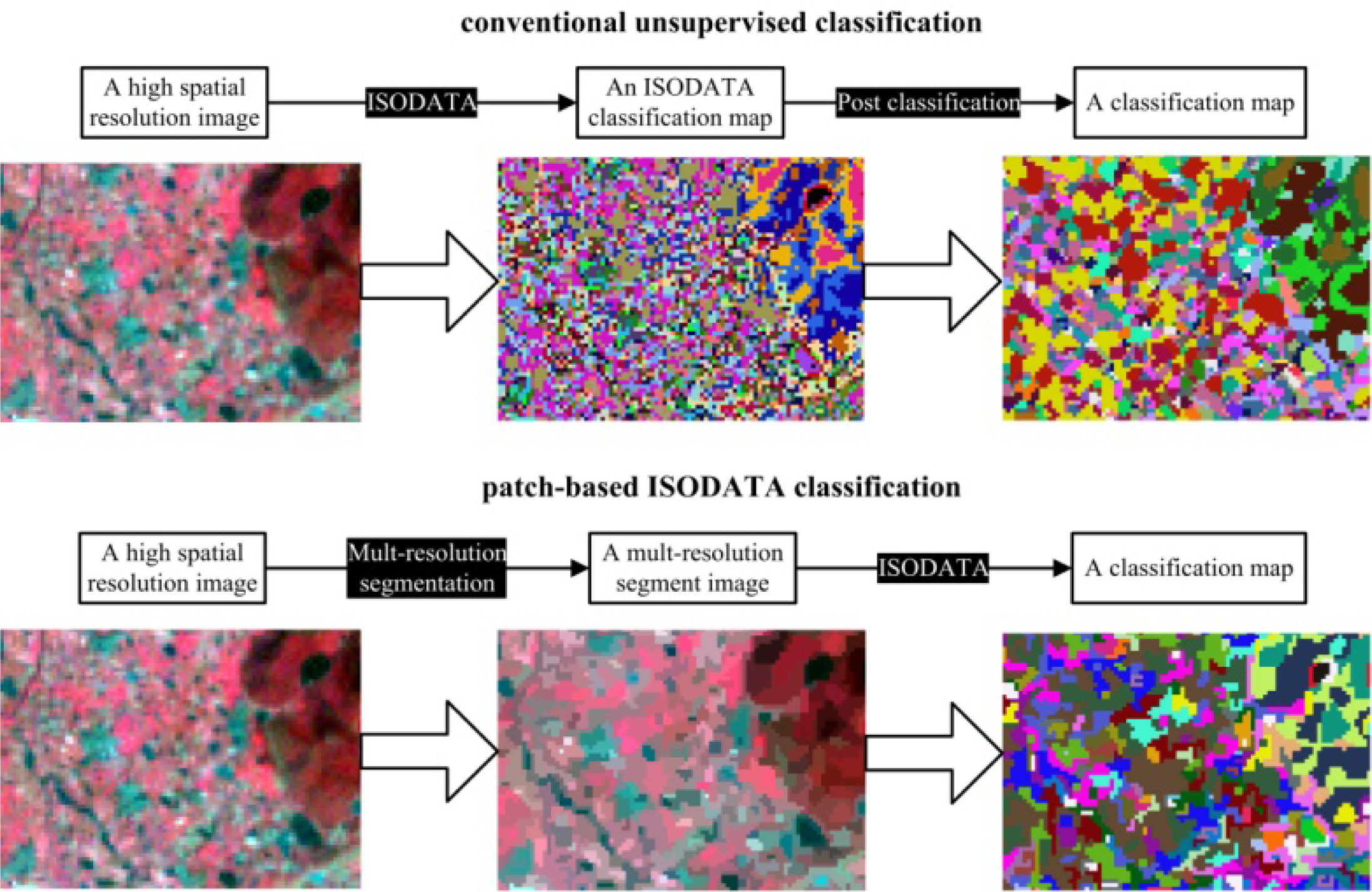
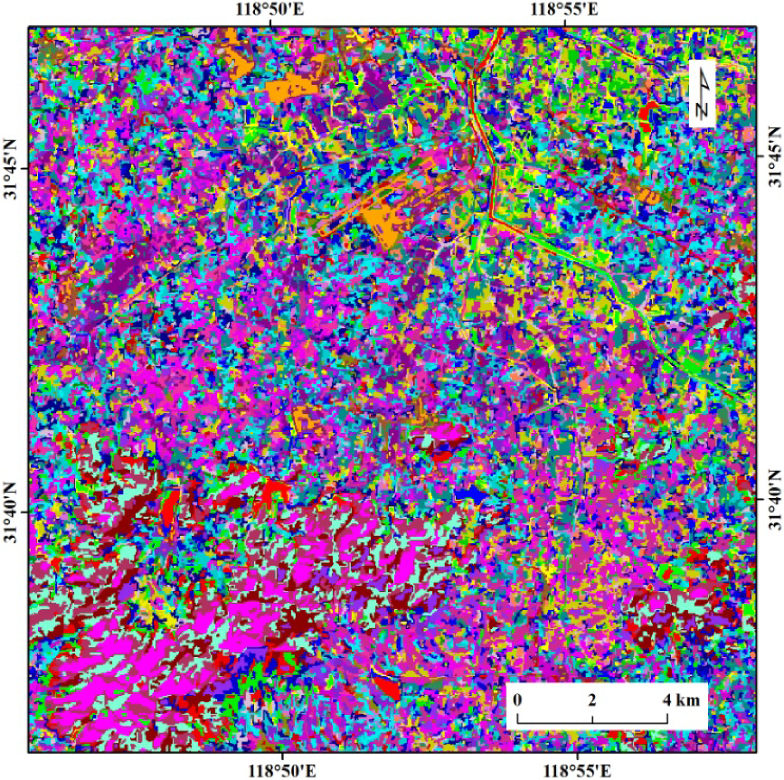
2.3.1. Patch-Based ISODATA Classification

The unmixing-based data fusion (e.g., STDFM or ESTDFM) needs a classification map with the HSRI(s) available. For this purpose, one generally uses an existing land-use map [14,18] or a map produced by performing a conventional unsupervised classification (e.g., ISODATA) [20,23]. However, the land-use map lacks timeliness and has fewer classes. In addition, the conventional unsupervised classification map usually meets the problem of how to deal with the “salt and pepper noise” well. This paper introduces a new classification method in which a key procedure of multi-resolution segmentation [24] is included (see Figure 1). Multi-resolution segmentation, one basic procedure for object-oriented image analysis, can segment the original single-pixel image into a homogenous-patch image, based on spectral, shape, and context information [25]. Thus, the negative influence coming from some small fraction objects (i.e., “salt and pepper noise”) [20,23] may be lowered when unmixing an LSRI based on a classification map gained by classifying an image consisting of homogenous patches (verified in detail in Section 5.2). Additionally, unlike the common object-oriented classification (e.g., fuzzy classification), the new method produces the classification map in an unsupervised way (e.g., ISODATA classification rule) (Figure 1), as it is not necessary to know the real class. Thus, the new classification method is named “patch-based ISODATA classification”.

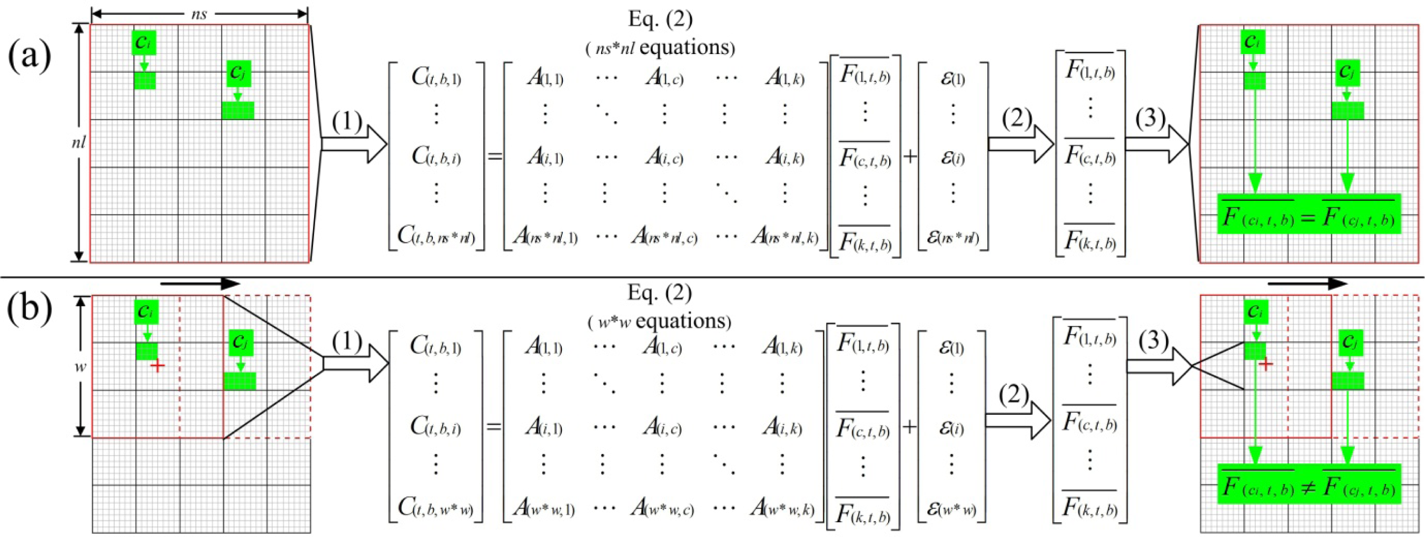
2.3.2. Sliding Window

Utilizing the information of all LSR pixels to create a linear system of equations (i.e., Equation (2)), and solving the unmixing for the whole LSRI, the STDFM algorithm can only get one reflectance value for all HSR pixels belonging to a same class (Figure 2a). Such an algorithm evidently rejects all the within-endmember variability [23], as the mean reflectance of endmembers in different LSR pixels may be dramatically different from each other over the whole LSRI. For example, even for crops growing in adjacent plots, their surface reflectance would be different due to environmental factors (e.g., illumination, soil type) or management practice (e.g., fertilization, harvest). For a whole image, the spatial heterogeneity will be more obvious. The ESTDFM algorithm applies the sliding window technology for such an improvement as: The mean reflectance of different endmembers in an LSR pixel is obtained through making use of the information of adjacent pixels in a certain window (e.g., w × w) (Figure 2b). Then, with reference to a classification map, the HSR pixels corresponding to the central target pixel (e.g., the LSR pixel labeled with a red cross in Figure 2b) are assigned the mean reflectance of different endmembers according to the rule that the HSR pixels belonging to the same endmember are assigned the same value. Finally, the whole LSRI can be unmixed in a sliding window, moved with the step of one LSR-pixel size (Figure 2b).

2.3.3. Temporal Weights

The STDFM algorithm acquires the predicted HSRI merely from the base HSRI at t₁, though two base HSRIs are available and two predicted results can be acquired. The ESTDFM algorithm adds the other predicted HSRI from the base HSRI at t₂ to make full use of the information of the base HSRIs. Thus, the final predicted HSRI at t₀ can be obtained by a temporal-weight combination of the two predicted results:

$$F_{(t0,b)}=T_{1(b)}\times F_{1(t0,b)}+T_{2(b)}\times F_{2(t0,b)}$$

(9)

where, F_1(t0,b) and F_2(t0,b) are, respectively, the predicted HSRIs from the base image at t₁ and t₂; T_1(b) and T_2(b) are, respectively, the temporal weights. Provided that the surface reflectance would experience more change along with the longer time interval, it would then be reasonable to simulate the different time intervals between the base date and the prediction date, according to the change magnitude detected by the LSR reflectance [11,13]:

$$T_{k(b)}=\frac{1/\left|\mathit{mean}(\sum _{j=1}^w\sum _{l=1}^{w}C\left(xj,yl,tk,b\right)-\sum _{j=1}^w\sum _{l=1}^{w}C\left(xj,yl,t0,b\right))\right|}{\sum _{k=1,2}1/\left|\mathit{mean}(\sum _{j=1}^w\sum _{l=1}^{w}C\left(xj,yl,tk,b\right)-\sum _{j=1}^w\sum _{l=1}^{w}C\left(xj,yl,t0,b\right))\right|}$$

(10)

where, x, y are the coordinates; w is the size of a sliding window; the other symbols are the same as above. The final predicted HSRI can be calculated by Equation (9), after the temporal weights are obtained.

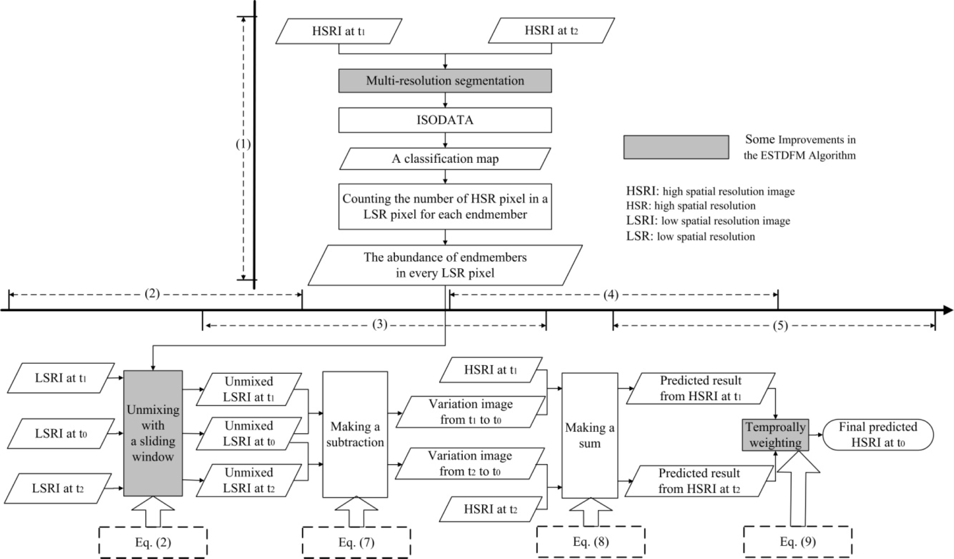
2.4. Process of the ESTDFM Algorithm Implementation

The ESTDFM algorithm is operated with the following steps as shown in Figure 3. Only two input image pairs at base dates (i.e., t₁ and t₂) and one input LSRI at prediction date (i.e., t₀) (time-series LSRIs can be used in practice) are used as an example. There are five major steps in the ESTDFM algorithm implementation (Figure 3). Firstly, the two HSRIs at base dates are used to get a classification map by performing a patch-based ISODATA classification; and the abundance of endmembers can be calculated based on the classification map. Secondly, the three LSRIs at base and prediction dates (i.e., t₁, t₂, and t₀) are, respectively, unmixed by a sliding window. Thirdly, two variation images are calculated by solving the difference between the unmixed LSRI at base date t₁, the unmixed one at base date t₂ and the unmixed one at prediction date (i.e., t₀) according to Equation (7). Fourthly, two predicted HSRIs can be obtained by making sums of the different base HSRIs and their corresponding variation images according to Equation (8). Finally, the two predicted HSRIs are temporally weighted to get the final HSRI at the prediction date according to Equation (9). The calculation method of temporal weights (i.e., Equation (10)) is described in detail in Section 2.3.3.

3. Algorithm Test

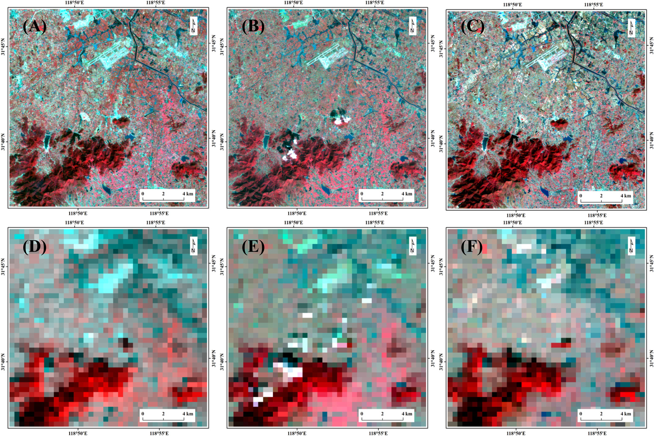
3.1. Test Data and Preprocessing

Three Landsat ETM+ images at 30 m spatial resolution and three corresponding MOD09GA images at a 500 m spatial resolution are selected as test data (see

Table 1. Test data for comparing the original algorithm and the proposed algorithm (i.e., Spatial and Temporal Data Fusion Model (STDFM) and Enhanced Spatial and Temporal Data Fusion Model (ESTDFM)).

Landsat ETM+			MOD09GA
Acquisition Date	Path/Row	Main Usage	Acquisition Date	Path/Row	Main Usage
10/08/02	120/38	Classification and validation	10/08/02	28/05	Unmixing
10/24/02	120/38	Validation	10/24/02	28/05	Unmixing
11/09/02	120/38	Classification	11/09/02	28/05	Unmixing

). The ETM+ and MOD09GA image pairs, from 8 October and 9 November, and the MOD09GA image, from 24 October, are used for the input data. The ETM+ image from 24 October is applied for validating the predicted results of different algorithms (i.e., STDFM and ESTDFM). Additionally, the ETM+ and MOD09GA image pair from 8 October is also employed for addressing if the patch-based ISODATA classification is more suitable for unmixing an LSRI than a conventional ISODATA classification. Since each Landsat multispectral reflectance band has a MODIS band with a similar bandwidth, ETM+ and MODIS land data (e.g., MOD09GA) have six corresponding bands (see

Table 2. Landsat Enhanced Thematic Mapper Plus (ETM+) bandwidth and Moderate Resolution Imaging Spectroradiometer (MODIS) land bandwidth. Three bands for testing are marked in bold.

ETM+ Band	Bandwidth (nm)	Spatial Resolution (m)	MODIS Land Band	Bandwidth (nm)	Spatial Resolution (m)
1	450–520	30	3	459–479	500
2	520–600	30	4	545–565	500
3	630–690	30	1	620–670	250a
4	760–900	30	2	841–876	250a
5	1,550–1,750	30	6	1,628–1,652	500
7	2,080–2,350	30	7	2,105–2,155	500

^aAlthough the spatial resolutions of band 1 and band 2 (i.e., red band and NIR band) in the standard MODIS daily surface reflectance data are 250 m, the spatial resolutions of all the six corresponding bands in MOD09GA are 500 m, as red and NIR bands are aggregated from the 250-m resolution in MOD09GA.

). However, it should be noted that the ESTDFM algorithm processes corresponding surface reflectance data, band by band, as described in Section 2, and this paper only selects three corresponding bands (i.e., red, green, and NIR bands) for testing.

All data are downloaded from USGS GLOVIS portal ( http://glovis.usgs.gov/). As the ETM+ data in the test have high geo-correction precision (the registration accuracies (RMS error) for the three Landsat scenes are, respectively, 2.94 m, 3.11 m, and 2.70 m), only radiation correction, including radiation calibration and atmospheric correction, is made for them. The correction procedure uses the Landsat ecosystem disturbance adaptive processing system (LEDAPS) [26] to convert DN values to surface reflectance. The MOD09GA data are reprojected from the native Sinusoidal projection to the UTM_WGS84 coordinate system, and resampled from 500 m to 480 m by means of the MODIS Reprojection Tool (MRT) to facilitate the subsequent calculation, as they are, exactly, the standard surface reflectance product with high-precision geolocation (approximately 50 m at NADIR) [27].

This paper selects an overlap region of MOD09GA and ETM+ data as the test area (see Figure 4). The region is located in the south of Nanjing, Jiangsu province, and covers an area of about 19 km × 19 km. It mostly contains cultivated lands and spreads over multiple kinds of ground objects: A river crosses over its upper right part; a plot of buildings is located in its upper middle part; and a piece of woodland and some small water pools are included in the lower left part. The river is hardly recognized on the MOD09GA image due to the coarse spatial resolution (Figure 4D–F).

3.2. Implementation Considerations

3.2.1. Patch-Based ISODATA Classification Map

At least two pairs of high- and low-spatial resolution images, acquired at two base dates, and one LSRI, acquired at prediction date, in the ESTDFM algorithm. Considering, if two ETM+ images are available, a more reasonable scheme for obtaining a classification map is to stack all bands of the two HSRIs and to classify the stacked HSRI. Therefore, according the process of patch-based ISODATA classification stated in Section 2.3.1, the specific steps for producing the classification map in the test are as follows: Firstly, all bands of the two ETM+ images (green, red, and NIR bands are tested in this paper) are stacked to generate a stacked image. Secondly, a segment image can be acquired by segmenting the stacked image (six bands in total) in the Ecognition software ( http://www.ecognition.com/) (scale parameter is empirically set as 20). Thirdly, only the mean reflectance of every object in the segment image is exported and converted to a grid image, though it has many characteristic values (e.g., mean, variance and peakness). Thus, the original image consisting of single pixels is converted to be an image consisting of homogeneous patches. Finally, a classification map with 40 classes (see Figure 5, the definition of the number of classes is described in Section 5.3), which is used for unmixing the three MOD09GA images, can be obtained by performing an ISODATA classification rule to the “patches image”.

3.2.2. Calculation of the Abundance of Endmembers

Based on the patch-based ISODATA classification map, the abundance of endmember, c, in a MOD09GA pixel can be calculated as:

$$A(c)=n_c/N$$

(11)

where, n_c is the number of ETM+ pixels belonging to endmember c in a MOD09GA pixel; N is the total number of ETM+ pixels contained in the MOD09GA pixel. As the pixel sizes of ETM+ and MOD09GA are, respectively, 30 m and 480 m in this paper, N is calculated to 256 (i.e., 16 × 16).

The calculated abundance of endmembers would be unchanged, assuming that the classification map is unchanged within the prediction period. In this case, it can be applicable to unmix the MOD09GA images at three dates (i.e., t₁, t₂ and t₀).

3.2.3. Unmixing of the MOD09GA Images

Since the abundance of endmembers has been known, three unmixed MOD09GA images can be acquired by applying the sliding window technology described in Section 2.3.2. There are two parameters to be optimized for unmixing an MOD09GA image in a sliding window. They are the number of classes contained in the classification map (n_e) and the size of sliding window (w). n_e can be given a higher value for a heterogeneity area than a homogeneous one. w is dialectically valued: On one hand, w should be given a low value to expand the spatial variation among the mean reflectance of endmembers in the unmixed image; on the other hand, w should be given a high value to establish adequate equations for unmixed stability [23]. Normally, both n_e and w have certain limitations. The quality of the unmixed image will be decreased when n_e and w are higher than their limitations. In this paper, “ERGAS” [28], a common comprehensive evaluation index for assessing the quality of an unmixed image, is employed to screen the optimal parameter combination (n_e = 40, w = 61; the screening method is described in Section 5.3) for unmixing the three MOD09GA images:

$$\mathit{ERGAS}=100\frac{h}{l}\sqrt{\frac{1}{nb}\sum _{i=1}^{nb}{{\mathit{RMSE}}_i}^2/{M_i}^2}$$

(12)

where, h is the pixel size of HSRI (30 m herein); l is the pixel size of LSRI (480 m herein); nb is the number of spectral bands (three or six herein); RMSE_i is the root-mean-square error of a certain band i, between the unmixed image and the reference image; M_i is the mean value of band i in the reference image. The lower the ERGAS is, the better the quality of an unmixed image [23].

3.3. Evaluation Methods

Three methods are introduced to compare the prediction effects of different algorithms (i.e., STDFM and ESTDFM) from different levels. (1) Visual evaluation. A visual comparison, one of common qualitative evaluation methods, between the predicted ETM+-like image and the actual ETM+ image, is made to roughly judge the prediction effect of an algorithm. (2) Scatter plots. The scatter plots for all corresponding bands between the actual image and the predicted one are used to semi-quantitatively describe the prediction effect of an algorithm. The closer to the line of 1:1 the scatters are, the better the prediction effect is. (3) Average absolute difference (AAD) value and average difference (AD) value. The AAD value is calculated for quantitatively presenting the prediction accuracy of an algorithm. In addition, the AD value is calculated for quantitatively making a description of the deviation (positive or negative) of a predicted result. For instance, that the AD value is positive implies the predicted result shows a positive deviation or a higher forecast; otherwise a negative deviation or a lower forecast. What is worthy of mentioning is that the STDFM algorithm tested in this paper applies the same classification method as ESTDFM (i.e., patch-based ISODATA classification) to get the classification map. Although a different classification method has been applied in the quoted literature (i.e., reference [16]), the essence of the STDFM algorithm in this paper is consistent.

4. Test Results of Algorithm

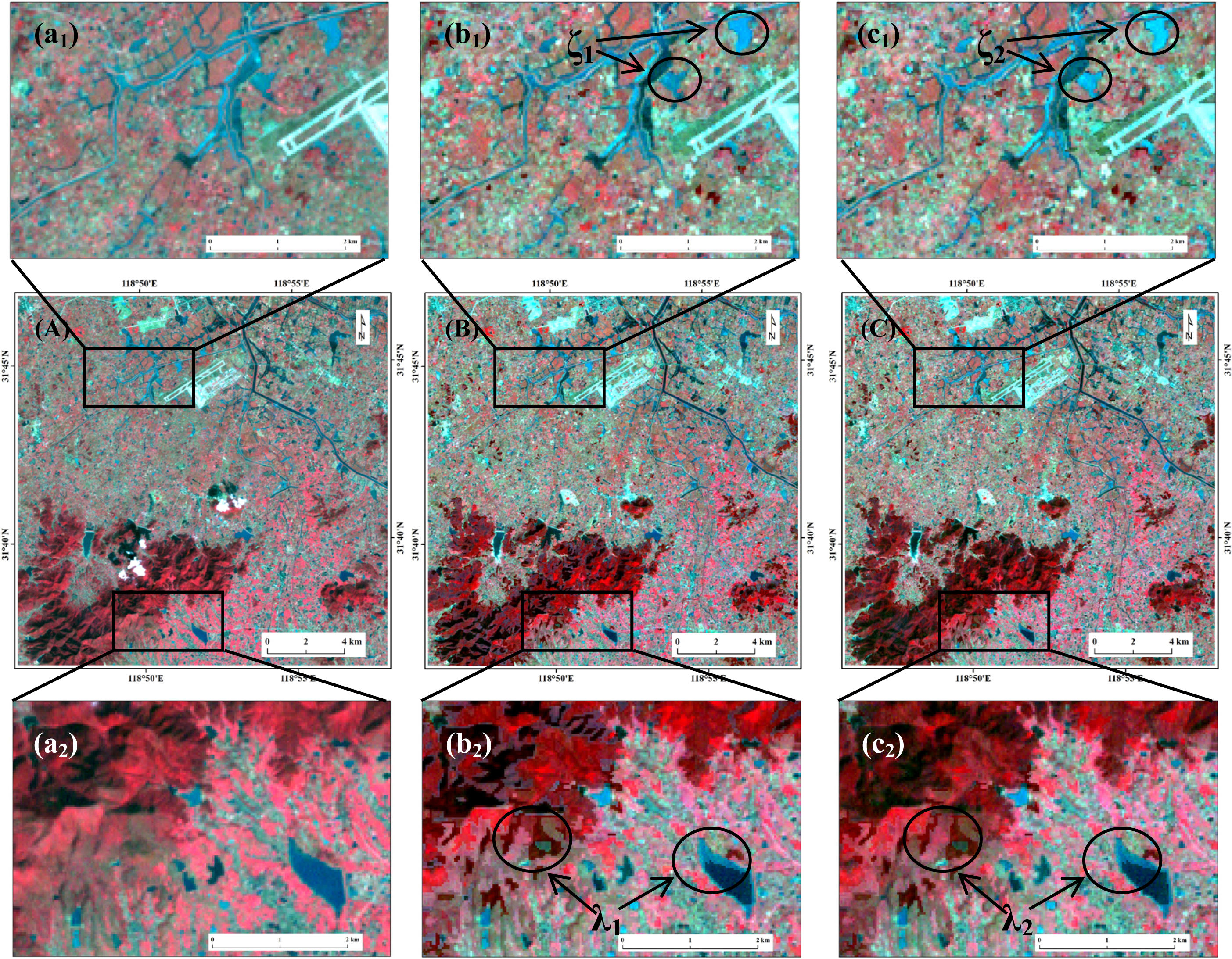
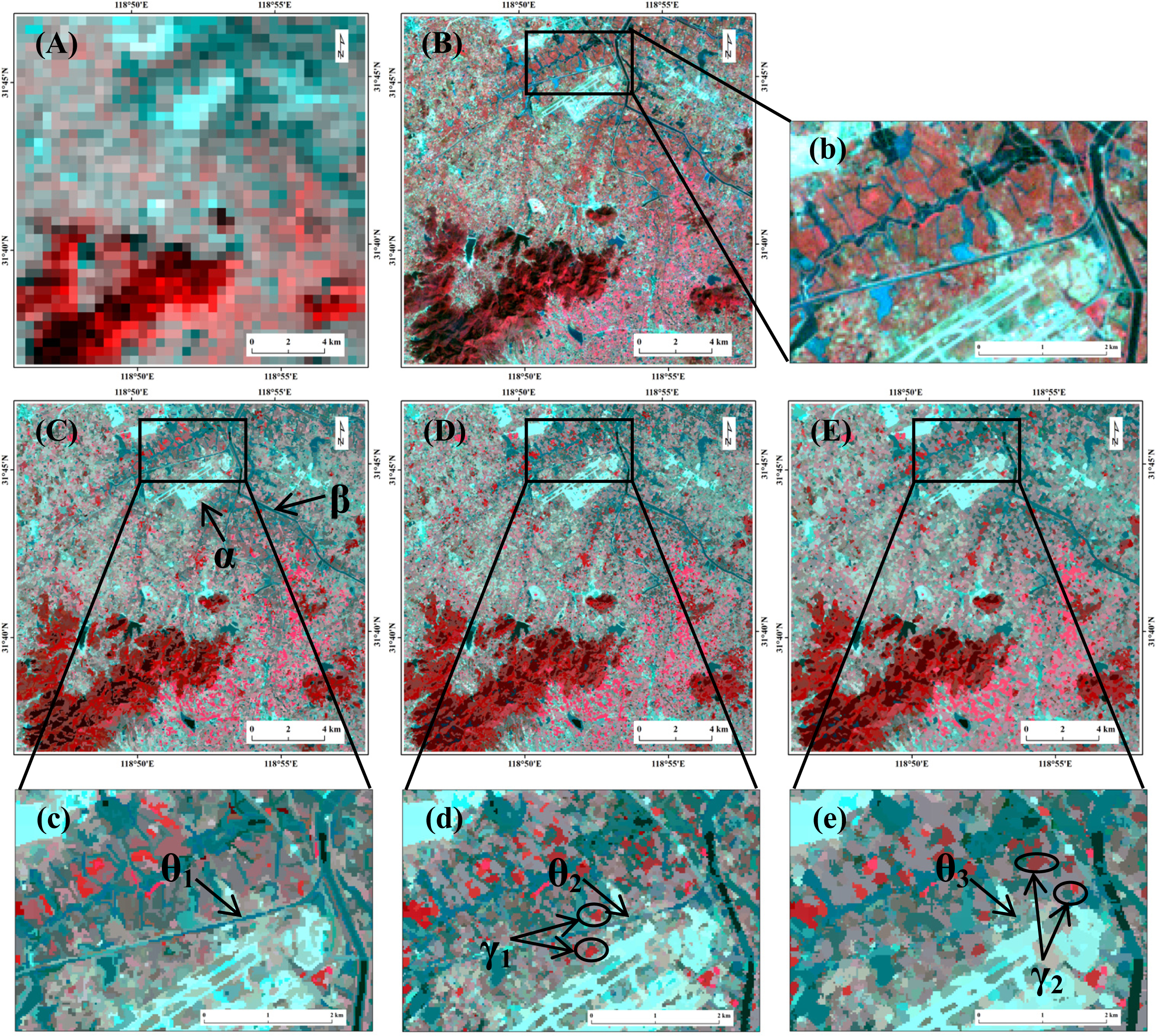
4.1. Visual Evaluation

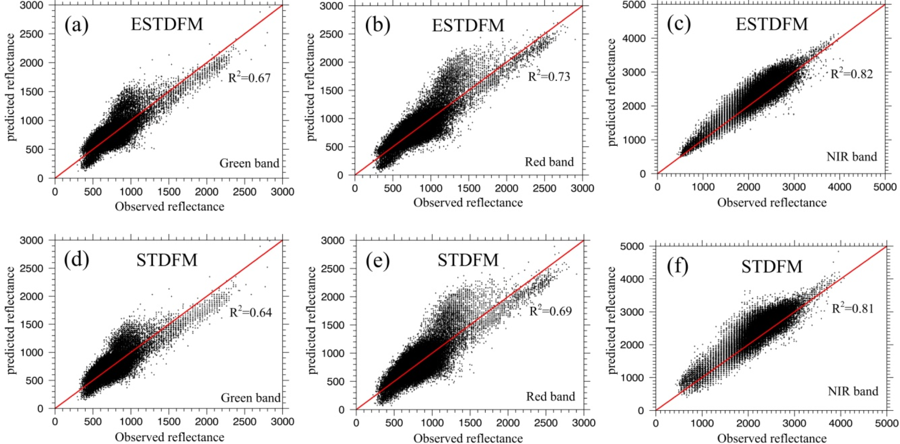
The ETM+-like images predicted by STDFM and ESTDFM are shown in Figure 6. Both algorithms can exactly retrieve the buildings, cultivated lands, woodlands, and so on, as their outlines are clearly seen. The predicted images are very close to the actual ones even watched in the partial enlarged details (Figure 6b₁ vs. Figure 6a₁; Figure 6c₁ vs. Figure 6a₁). However, some undesired cases still appear. For example, a bit of clouds in the actual ETM+ image are not presented in both of the predicted images (Figure 6B vs. Figure 6A; Figure 6C vs. Figure 6A). As clouds are transient and not recorded in the classification map, the cloud pixels will be assigned the same reflectance as other classes (e.g., cultivated lands) in the unmixing of the MOD09GA images, which causes the disappearance of clouds in the predicted image. Additionally, some errors emerge in the forecasts of dense vegetation (e.g., some forests and croplands) where the hue is in a deeper red than the observations (Figure 6B vs. Figure 6A; Figure 6C vs. Figure 6A). Nevertheless, for some water areas (e.g., ζ₁ vs. ζ₂ in Figure 6), ESTDFM makes a more accurate prediction, as the prediction of STDFM seems “brighter” than the real image.

4.2. Scatter Plots

The scatter plots in Figure 7 show the relationship between the reflectance of the actual ETM+ image on 24 October and the reflectance of the predicted images with different algorithms for green band, red band, and NIR band, respectively. Similar to the visual evaluation, the scatters of all bands distribute closely to the line of 1:1, indicating that both algorithms can make a good prediction for an unknown HSRI. For the green band and the red band, the forecasts of ESTDFM are slightly better than the ones of STDFM (Figure 7a) vs. Figure 7d; Figure 7b vs. Figure 7e). However, for the NIR band, the forecast of ESTDFM is much better than the one from STDFM, as the former’s scatters are, not only closer to the line of 1:1, but also have no evident deviation; while most of the latter’s scatters are obviously higher than the line of 1:1 (Figure 7c vs. Figure 7f). The contrasting results can be also proven in the visual check of Figure 6 (e.g., ζ₁ vs. ζ₂ in Figure 6).

4.3. AAD and AD

Table 3. Average Absolute Difference (AAD) values and Average Difference (AD) values between the observed reflectance at two base dates (8 October 2002 and 9 November 2002), the predicted reflectance for 24 October 2002 by different algorithms (ESTDFM or STDFM) and the observed reflectance on 24 October 2002.

ETM+	AAD				AD
Band	Base Date1	Base Date2	Prediction		Base Date1	Base Date2	Prediction
	10/08/02	11/09/02	ESTDFM	STDFM	10/08/02	11/09/02	ESTDFM	STDFM
Green	0.0081	0.0110	0.0073	0.0078	0.0014	0.0089	0.0006	0.0010
Red	0.0111	0.0212	0.0090	0.0102	0.0001	0.0202	0.0012	0.0013
NIR	0.0475	0.0191	0.0167	0.0265	0.0474	−0.0112	0.0130	0.0243

shows the AAD and the AD values between the reflectance of the base ETM+ images from 8 October and 9 November, the predicted reflectance for 24 October and the reflectance of the ETM+ image from 24 October. The AAD values of both algorithms are lower than the ones of the base ETM+ images for all bands (Table 3), indicating that both algorithms successfully integrate the surface reflectance change of MOD09GA images into the base ETM+ images. The forecasts of the two algorithms for the green band and the red band are similar and have no evident deviation (green-AD: 0.0006 vs. 0.0010; red-AD: 0.0012 vs. 0.0013), although the prediction errors of ESTDFM are a little lower than those of STDFM (green-AAD: 0.0073 vs. 0.0078; red-AAD: 0.0090 vs. 0.0102). However, for the NIR band, the prediction errors of ESTDFM are remarkably lower than that of STDFM (NIR-AAD: 0.0167 vs. 0.0265) and both of their forecasts, obviously, have positive deviations, though the degree of former’s forecast is lower (NIR-AD: 0.0130 vs. 0.0243). A higher forecast for NIR band will cause a higher hue in “red channel” in the NIR-red-green composites of the predicted images. In addition, it is the reason why both algorithms have a deeper red hue in their forecasts of some dense vegetation in the visual evaluation (Figure 6B vs. Figure 6A; Figure 6C vs. Figure 6A). Generally, the prediction effect of ESTDFM is better than that of STDFM.

5. Discussions

5.1. Point Spread Function

As with some previous studies [16,18], the point spread function (PSF) [29,30] is not considered in the calculation of the abundance of endmembers, as mentioned in Section 3.2.2. The calculated abundance is actually the area proportion of each class within a certain LSR pixel. Nonetheless, this paper just focuses on anglicizing the two algorithms in a comparative way. That is, which one is better has nothing to do with the classification map and the abundance. Thus, it is appropriate to neglect the item. Surely, it will be better to consider it in some practical applications of the ESTDFM algorithm, as almost 25% signal of MODIS data comes from adjacent pixels [31].

5.2. Suitability of the New Classification Method

The MOD09GA and ETM+ image pair from 8 October 2002 (Figure 8A,B) is used for validating the superiority of the new classification method (i.e., patch-based ISODATA classification) for unmixing an LSRI. A combination of the ISODATA classification and the Majority Analysis post classification, a common unsupervised method, is set as a contrast to the new classification. A transfer kernel, where the class of central pixel will be replaced with the class of major pixels, is designated in the Majority Analysis post classification, so that the “salt and pepper noise” can be reduced. The kernels in different sizes (3 × 3 and 5 × 5) are set in the comparison tests. The scheme for validation is: Firstly, the different classification methods are performed to classify the ETM+ image from 8 October to produce their corresponding classification maps with the same number of classes (e.g., n_e = 40). Secondly, a set of sliding windows with different sizes (e.g., 11 × 11, 21 × 21, …, w × w) is applied to unmix the MOD09GA image from October 8, based on the different classification maps. Finally, the unmixed results are evaluated with qualitative (e.g., visual evaluation) and quantitative (e.g., ERGAS index) methods.

Figure 8 shows the unmixed images of the three methods with the optimal parameter combination (i.e., n_e = 40, w = 61). Both algorithms generally present good unmixing effects. The “salt and pepper noise” is effectively reduced so that no “abrupt” points appear in the unmixed images compared to the unmixed one, based on a map with no post classification (not shown here). In addition, their spatial resolutions are obviously finer than that of the original MOD09GA image. For instance, the residential area (α in Figure 8C) at the upper middle part and the river (β in Figure 8C) at the upper right part can be distinctly recognized, and the details of woodland at lower left part can be reflected completely (Figure 8C–E). However, the unmixed images of the two conventional unsupervised methods present some “clumps” (e.g., γ₁ in Figure 8d and γ₂ in Figure 8e), which are unmatched with the truth. In addition, the riverlet in the actual ETM+ image (Figure 8b) is reflected in varied degrees: The riverlet is continuous in Figure 8c (θ₁ in Figure 8c); however, its continuity is poorly shown in Figure 8d (θ₂ in Figure 8d); and it even disappears in Figure 8e (θ₃ in Figure 8e). The “clumps” phenomenon and the discontinuity of the riverlet in Figure 8d,e may be caused by the transfer kernel in the post classification, as the process is a mathematical calculation, which means that the real shape of an object is not considered, and the size of a transfer kernel may be larger than the width of the riverlet, which could “erase” the riverlet in the post classification. Generally, the new classification method can, not only reduce the “salt and pepper noise”, but also obtain an unmixed image closer to the real ground objects from the visual check.

According to Equation (12), by regarding the observed ETM+ image from October 8 as the reference image and regarding the unmixed results based on the different classification maps as the unmixed images, the ERGAS values are calculated and recorded as ERGAS_H. The lower the ERGAS_H is, the closer the attribute of spatial resolution of an unmixed image is to the reference image, and the better the quality of an unmixing image is to some degrees [23]. The quantitative results (i.e., ERGAS_H values) are summarized in

Table 4. ERGAS_H values of the different classification methods for unmixing MOD09GA images from 8 October 2002 with different sizes of sliding windows.

	w	11	21	31	41	51	61
Method
patch-based ISODATA classification		1.89	1.46	1.33	1.29	1.26	1.24
Majority Analysis1 (3 × 3) a		2.18	1.60	1.41	1.33	1.29	1.27
Majority Analysis2 (5 × 5) b		1.87	1.49	1.39	1.36	1.34	1.33
No Post Classification c		5.12	2.48	2.15	2.03	1.97	1.96

^aThe ISODATA classification and the Majority Analysis post classification with a 3 × 3 transfer kernel are included in the method;

^bThe ISODATA classification and the Majority Analysis post classification with a 5 × 5 transfer kernel are included in the method;

^cOnly the ISODATA classification (no post classification for filtering noise) is included in the method.

. All the ERGAS_H values of the three methods are lower than those of the method with no post classification (Table 4), indicating that the classification maps gained from the new classification, or an ISODATA classification including a post classification, can improve the quality of an unmixing image. In addition, all the ERGAS_H values of the three methods are lower than 3, stating quantitatively that all the unmixed images based on them show good qualities [32]. The two noteworthy points are that all ERGAS_H values have an obvious trend of “better in wider window” and that the ERGAS_H values of the new classification method are almost minimal in all sliding-window sizes (except for k = 11, see Table 4), which expressly proves that the new classification method is more suitable for unmixing an LSRI, compared to the other conventional unsupervised classification methods.

The original single-pixel image can be segmented into a homogeneous-patch image by means of multi-resolution segmentation, according to the information of spectrum, spatial location, and shape among pixels. On one hand, the classification accuracy may not be influenced greatly, since the difference between homogeneous patches is retained in the process of multi-resolution segmentation [24]; on the other hand, unlike using a mathematical method (e.g., transfer kernel) to eliminate the “salt and pepper noise” in a conventional unsupervised classification, the patch-based ISODATA classification has considered multiple factors in multi-resolution segmentation to get a segment image [25], which may be more of a benefit for both “salt and pepper de-noising” and fidelity to real objects.

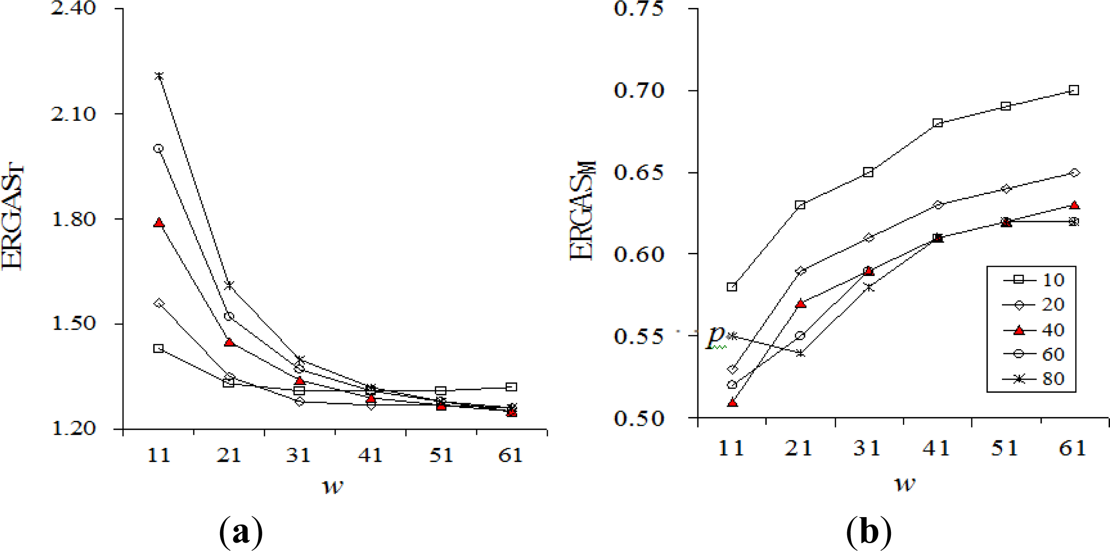
5.3. Definition of Optimal Parameter Combination

As mentioned in Section 3.2.2, the class number (n_e) and the size of sliding window (w) will exert direct impacts on the unmixing effect. The two necessary input image pairs (e.g., the ETM+ and MOD09GA image pairs from 8 October and 9 November in the paper) in the ESTDFM algorithm are used to calculate two ERGAS indexes (ERGAS_T and ERGAS_M) for screening the optimal parameter combination. ERGAS_T: Firstly, the two ETM+ images and the two MOD09GA images, at two base dates, are stacked, respectively. Secondly, a set of parameter combinations is applied to unmix the stacked MOD09GA image (six bands in total). Finally, according to Equation (12), by taking the stacked ETM+ image (six bands in total) as the reference image, and taking the unmixed stacked MOD09GA images as the unmixed images, the ERGAS values are calculated and recorded as ERGAS_T. ERGAS_M: A mean filter is used to degrade the unmixed stacked MOD09GA images to the same spatial resolution as a MOD09GA image (i.e., 480 m). Then, by taking the stacked MOD09GA image (six bands in total) as the reference image and taking the degraded images as the unmixed images, the ERGAS values are calculated and recorded as ERGAS_M.

The ERGAS_T (Figure 9a) and the ERGAS_M (Figure 9b) for all parameter combinations show almost opposite trends to each other. For instance, when n_e = 40 and w is enlarged from 11 to 61, the ERGAS_T is valued from 1.79 down to 1.25 (red triangle in Figure 9a); while the ERGAS_M is valued from 0.51 up to 0.63 (red triangle in Figure 9b). It indicates that there is no such parameter combination can make both indices reach the minimum simultaneously. In deliberation of the trends of both indices from all perspectives, the combination of n_e = 40 and w = 61 is selected as the optimal parameter combination for unmixing the MOD09GA images in this paper. Additionally, there is an obvious exceptional point, p, in Figure 9b. It might be relative to the instability in the unmixing process when n_e is high (e.g., 80) while w is low (e.g., 11). In that case, the unmixing equations in Equation (2) are relatively in smaller quantities.

It may be unbalanced to assess the unmixing effects by only applying ERGAS_T. As ERGAS_T values become lower with the expansion of window size (Figure 9a), the unmixing effect seems to be better when the window is larger from the angle of the ERGAS_T trend. However, the expansion of the window size will cause the problem that the spatial variation of mean reflectance will be inevitably brought down. Thus, it is not straightforward to define the optimal parameter combination. Meanwhile, unmixing an LSRI can be regarded as the process of redistribution of energy in terms of the energy conservation. Assuming that the energy between the unmixed image and the original LSRI should be well “balanced” [20], ERGAS_M index can be recommended for making a quantitative assessment on the energy redistribution process. As all the energy of the unmixed image comes from the original LSRI, ERGAS_M being low means the unmixed image “maintains” the original energy; otherwise, loses. Thus, the optimal parameter combination is screened on the condition that ERGAS_T has to be very low, firstly, and ERGAS_M must not be too high, secondly. In actuality, it is a semi-quantitative scheme. The different optimal parameter combinations could be defined according to the different practical needs (e.g., focusing on the high-spatial resolution characteristic or the energy conservation characteristic).

5.4. Drawbacks in the ESTDFM Algorithm

5.4.1. “Patch Effect”

Similar to the original STDFM algorithm, one of the drawbacks in the ESTDFM algorithm is the undesired “patch effect” in the predicted result (λ₁ and λ₂ in Figure 6). It may be related to the classification map. According to the process of unmixing an LSRI stated in Section 2.3.2, the HSR pixels belonging to a same class are assigned the same reflectance. Therefore, the unmixed image is directly influenced by the classification map, so that the “class effect” (see Figure 8c,d,e) is always visible. Subsequently, two cases that can result in “patch effect” may emerge. Case (1) for the different sections of one patch: The base reflectance value (i.e., F_(c,tk,b) in Equation (6)) in different sections of one patch is very close as they belong to a same class. However, they may be located in different LSR pixels, which will lead to different variation of reflectance (i.e., $\mathrm{\Delta }\overline{F_{(c,\mathrm{\Delta }{t}_k,b)}}$ in Equation (6)). Thus, the predicted results, the sums of the base reflectance and the variation of reflectance, in those sections may become different, which may disrupt the spatial continuity. Case (2) for the neighbor patches: The neighbor patches may have very different base reflectance and variation of reflectance if they belong to different classes, which is more likely to disrupt the spatial continuity. The promising method for reducing the “patch effect” may be the soft clustering classification method [33] presented in the recent studies [34,35], and applied in some cases with good performance.

5.4.2. Time Consumption

There are five major steps in the implementation of the ESTDFM algorithm (see Section 2.4). However, it takes a little time for the processes of Step 1 (i.e., Classification), Step3 (i.e., Subtraction), Step4 (i.e., Sum) and Step5 (i.e., Temporally-weighted Sum). The Step 2 (i.e., Unmixing) requires most time. Thus, we compare the time consumption of unmixing an LSRI in the two algorithms. Results show that the time consumption of ESTDFM is longer than that of STDFM (about 88 s vs. 25 s) for unmixing one LSR band with 100 × 100 pixels (i.e., 48 km × 48 km), running at a common desktop computer (2 CPU, 2.66 GHz, 4 G RAM). It takes about 20 min to unmix one LSR band of which the area is almost equal to a range of a Landsat scene (i.e., about 180 km × 180 km). We believe that the computation time cost of the proposed algorithm is acceptable.

5.4.3. Constraints

Extra attention may need to be paid. Firstly, the rationality of the theoretical basis of ESTDFM (i.e., the linear spectral fusion model) is still under discussion [36]. Secondly, the determination of relevant parameters is not strictly regulated. For example, the scale parameter in multi-resolution segmentation, the class number (n_e), and the size of sliding window (w), are defined with an empirical or semi-quantitative method. Thirdly, the assumption that the classification map is unchanged in the forecast period could be reasonable in a short term, but unreasonable in a long time. The prediction effect may be worse in a longer forecast period. Finally, as with some other fusion algorithms for predicting high temporal Landsat-like data (e.g., STARFM in Gao et al. [11] and ESTARFM in Zhu et al. [13]), if changes are transient and not recorded in any of the base Landsat images (e.g., clouds), it may not be possible to capture them in a fine resolution.

6. Conclusions and Summary

The enhanced STDFM (ESTDFM) algorithm has improved the STDFM algorithm by introducing a patch-based ISODATA classification method, the sliding window technology, and the temporal-weight concept. Tests have proved that the ESTDFM algorithm can acquire a more accurate forecast than the original STDFM algorithm (e.g., the contrasting average absolute differences for NIR band: 0.0167 vs. 0.0265). The progresses of the ESTDFM algorithm are summarized below:

(1)

The most important improvement in the ESTDFM algorithm is to apply a sliding widow for unmixing a low spatial resolution image (LSRI). Only one reflectance value for each endmember can be obtained in the unmixing of an LSRI in the original STDFM algorithm, as all low spatial resolution (LSR) pixels are unmixed at once. Obviously, such an algorithm rejects all the within-endmember variability. By introducing the sliding widow technology, the ESTDFM algorithm unmixes the adjacent pixels in a window to get the mean reflectance of different endmembers, and assigns them to the HSR pixels corresponding to the central target LSR pixel with reference to a classification map; subsequently unmixes all LSR pixels by a sliding window, moved with the step of one LSR-pixel size. The spatial heterogeneity of the mean reflectance of endmembers has been fully considered, which would be more consistent with the variation of real ground objects.

(2)

The temporal-weight concept is introduced in the ESTDFM algorithm. One predicted high spatial resolution image (HSRI) can be acquired, by making a sum of one base HSRI and its corresponding variation image calculated by solving a difference between the unmixed LSRI at base date and the unmixed one at prediction date. Therefore, two different predicted HSRIs can be obtained, as two high- and low-spatial resolution image pairs at base date, and one LSRI at prediction date, are available in the ESTDFM algorithm. Thus, making full use of the information of the known HSRIs, a more reasonable scheme to obtain the final predicted HSRI is temporally weighting the two predicted results.

(3)

A patch-based ISODATA classification method is also introduced in the ESTDFM algorithm. Two main procedures are included in the method: A single-pixel HSRI is firstly converted into a homogeneous-patch image base on multi-resolution segmentation. A patch-based ISODATA classification map then can be acquired by applying the ISODATA classification rule to the “patches image”. Test results show that the new classification method is more suitable for unmixing an LSRI than some conventional unsupervised classification methods, since an unmixed LSRI based on a patch-based ISODATA classification map not only has low “salt and pepper noise” but is more consistent with the real object.

Compared with the original STDFM algorithm, the proposed algorithm can generally fuse the multi-sourced data with different characteristics in a short-time period better to generate the remotely sensed data with high temporal and spatial resolutions. However, the ESTDFM algorithm still has some drawbacks (e.g., “patch effect”) and constraints (e.g., the linear spectral fusion model), as well as more time consumption. The proposed method will push forward the studies of monitoring the land surface dynamic changes at finer scales by remote sensing technology.

References

1. Price, J.C. How unique are spectral signatures? Remote Sens. Environ 1994, 49, 181–186. [Google Scholar]
2. Sakamoto, T.; van Nguyen, N.; Ohno, H.; Ishitsuka, N.; Yokozawa, M. Spatio-temporal distribution of rice phenology and cropping systems in the Mekong Delta with special reference to the seasonal water flow of the Mekong and Bassac rivers. Remote Sens. Environ 2006, 100, 1–16. [Google Scholar]
3. Notarnicola, C.; Duguay, M.; Moelg, N.; Schellenberger, T.; Tetzlaff, A.; Monsorno, R.; Costa, A.; Steurer, C.; Zebisch, M. Snow cover maps from MODIS images at 250 m resolution, Part 1: Algorithm description. Remote Sens 2013, 5, 110–126. [Google Scholar]
4. Zhou, H.; Aizen, E.; Aizen, V. Deriving long term snow cover extent dataset from AVHRR and MODIS data: Central Asia case study. Remote Sens. Environ 2013, 136, 146–162. [Google Scholar]
5. Rees, W.; Williams, M.; Vitebsky, P. Mapping land cover change in a reindeer herding area of the Russian Arctic using Landsat TM and ETM+ imagery and indigenous knowledge. Remote Sens. Environ 2003, 85, 441–452. [Google Scholar]
6. Lier, O.R.V.; Luther, J.E.; Leckie, D.G.; Bowers, W.W. Development of large-area land cover and forest change indicators using multi-sensor Landsat imagery: Application to the Humber River Basin, Canada. Int. J. Appl. Earth Obs. Geoinf 2011, 13, 819–829. [Google Scholar]
7. Santillan, J.; Makinano, M.; Paringit, E. Integrated Landsat image analysis and hydrologic modeling to detect impacts of 25-year classification change on surface runoff in a Philippine watershed. Remote Sens 2011, 3, 1067–1087. [Google Scholar]
8. Marfai, M.A.; Almohammad, H.; Dey, S.; Susanto, B.; King, L. Coastal dynamic and shoreline mapping: Multi-sources spatial data analysis in Semarang Indonesia. Environ. Monit. Assess 2008, 142, 297–308. [Google Scholar]
9. Hilker, T.; Wulder, M.A.; Coops, N.C.; Linke, J.; McDermid, G.; Masek, J.G.; Gao, F.; White, J.C. A new data fusion model for high spatial-and temporal-resolution mapping of forest disturbance based on Landsat and MODIS. Remote Sens. Environ 2009, 113, 1613–1627. [Google Scholar]
10. Arai, E.; Shimabukuro, Y.E.; Pereira, G.; Vijaykumar, N.L. A multi-resolution multi-temporal technique for detecting and mapping deforestation in the Brazilian Amazon rainforest. Remote Sens 2011, 3, 1943–1956. [Google Scholar]
11. Gao, F.; Masek, J.; Schwaller, M.; Hall, F. On the blending of the Landsat and MODIS surface reflectance: Predicting daily Landsat surface reflectance. IEEE Trans. Geosci. Remote Sens 2006, 44, 2207–2218. [Google Scholar]
12. Hilker, T.; Wulder, M.A.; Coops, N.C.; Seitz, N.; White, J.C.; Gao, F.; Masek, J.G.; Stenhouse, G. Generation of dense time series synthetic Landsat data through data blending with MODIS using a spatial and temporal adaptive reflectance fusion model. Remote Sens. Environ 2009, 113, 1988–1999. [Google Scholar]
13. Zhu, X.; Chen, J.; Gao, F.; Chen, X.; Masek, J.G. An enhanced spatial and temporal adaptive reflectance fusion model for complex heterogeneous regions. Remote Sens. Environ 2010, 114, 2610–2623. [Google Scholar]
14. Zurita-Milla, R.; Kaiser, G.; Clevers, J.; Schneider, W.; Schaepman, M. Downscaling time series of MERIS full resolution data to monitor vegetation seasonal dynamics. Remote Sens. Environ 2009, 113, 1874–1885. [Google Scholar]
15. Zurita-Milla, R.; Clevers, J.; van Gijsel, J.; Schaepman, M. Using MERIS fused images for classification mapping and vegetation status assessment in heterogeneous landscapes. Int. J. Remote Sens 2011, 32, 973–991. [Google Scholar]
16. Wu, M.; Wang, J.; Niu, Z.; Zhao, Y.; Wang, C. A model for spatial and temporal data fusion (In Chinese). J. Infrared Millim. Waves 2012, 31, 80–84. [Google Scholar]
17. Maselli, F. Definition of spatially variable spectral endmembers by locally calibrated multivariate regression analyses. Remote Sens. Environ 2001, 75, 29–38. [Google Scholar]
18. Busetto, L.; Meroni, M.; Colombo, R. Combining medium and coarse spatial resolution satellite data to improve the estimation of sub-pixel NDVI time series. Remote Sens. Environ 2008, 112, 118–131. [Google Scholar]
19. Minghelli-Roman, A.; Polidori, L.; Mathieu-Blanc, S.; Loubersac, L.; Cauneau, F. Spatial resolution improvement by merging MERIS-ETM images for coastal water monitoring. IEEE Geosci. Remote Sens. Lett 2006, 3, 227–231. [Google Scholar]
20. Zhukov, B.; Oertel, D.; Lanzl, F.; Reinhackel, G. Unmixing-based multisensor multiresolution image fusion. IEEE Trans. Geosci. Remote Sens 1999, 37, 1212–1226. [Google Scholar]
21. Settle, J.; Drake, N. Linear mixing and the estimation of ground cover proportions. Int. J. Remote Sens 1993, 14, 1159–1177. [Google Scholar]
22. Oleson, K.; Sarlin, S.; Garrison, J.; Smith, S.; Privette, J.; Emery, W. Unmixing multiple classification type reflectances from coarse spatial resolution satellite data. Remote Sens. Environ 1995, 54, 98–112. [Google Scholar]
23. Zurita-Milla, R.; Clevers, J.; Schaepman, M.E. Unmixing-based Landsat TM and MERIS FR data fusion. IEEE Geosci. Remote Sens. Lett 2008, 5, 453–457. [Google Scholar]
24. Baatz, M.; Schape, A. Multiresolution Segmentation—An Optimization Approach for High Quality Multi-Scale Image Segmentation. In Angewandte Geographische Informations-Verarbeitung XII; Strobl, J., Blaschke, T., Griesebner, G., Eds.; Wichmann Verlag: Karlsruhe, Germany, 2000; pp. 12–23. [Google Scholar]
25. Benz, U.C.; Hofmann, P.; Willhauck, G.; Lingenfelder, I.; Heynen, M. Multi-resolution, object-oriented fuzzy analysis of remote sensing data for GIS-ready information. ISPRS J. Photogramm. Remote Sens 2004, 58, 239–258. [Google Scholar]
26. Masek, J.G.; Vermote, E.F.; Saleous, N.E.; Wolfe, R.; Hall, F.G.; Huemmrich, K.F.; Gao, F.; Kutler, J.; Lim, T.-K. A Landsat surface reflectance dataset for North America, 1990–2000. IEEE Geosci. Remote Sens. Lett 2006, 3, 68–72. [Google Scholar]
27. Wolfe, R.E.; Nishihama, M.; Fleig, A.J.; Kuyper, J.A.; Roy, D.P.; Storey, J.C.; Patt, F.S. Achieving sub-pixel geolocation accuracy in support of MODIS land science. Remote Sens. Environ 2002, 83, 31–49. [Google Scholar]
28. Wald, L. Quality of High Resolution Synthesized Images: Is There a Simple Criterion? Proceedings of the International Conference Fusion of Earth Data, Sophia Antipolis, France, 26–28 January 2000; pp. 99–103.
29. Townshend, J.; Huang, C.; Kalluri, S.; Defries, R.; Liang, S.; Yang, K. Beware of per-pixel characterization of land cover. Int. J. Remote Sens 2000, 21, 839–843. [Google Scholar]
30. Huang, C.; Townshend, J.R.; Liang, S.; Kalluri, S.N.; DeFries, R.S. Impact of sensor’s point spread function on land cover characterization: Assessment and deconvolution. Remote Sens. Environ 2002, 80, 203–212. [Google Scholar]
31. Tan, B.; Woodcock, C.; Hu, J.; Zhang, P.; Ozdogan, M.; Huang, D.; Yang, W.; Knyazikhin, Y.; Myneni, R. The impact of gridding artifacts on the local spatial properties of MODIS data: Implications for validation, compositing, and band-to-band registration across resolutions. Remote Sens. Environ 2006, 105, 98–114. [Google Scholar]
32. Ranchin, T.; Aiazzi, B.; Alparone, L.; Baronti, S.; Wald, L. Image fusion—The ARSIS concept and some successful implementation schemes. ISPRS J. Photogramm. Remote Sens 2003, 58, 4–18. [Google Scholar]
33. Kohonen, T. Self-Organizing Maps, 3rd ed.; Springer-Verlag: New York, NY, USA, 2001. [Google Scholar]
34. Amorós-López, J.; Gomez-Chova, L.; Alonso, L.; Guanter, L.; Zurita-Milla, R.; Moreno, J.; Camps-Valls, G. Multitemporal fusion of Landsat/TM and ENVISAT/MERIS for crop monitoring. Int. J. Appl. Earth Obs. Geoinf 2013, 23, 132–141. [Google Scholar]
35. Amorós-López, J.; Gomez-Chova, L.; Alonso, L.; Guanter, L.; Moreno, J.; Camps-Valls, G. Regularized multiresolution spatial unmixing for ENVISAT/MERIS and Landsat/TM image fusion. IEEE Geosci. Remote Sens. Lett 2011, 8, 844–848. [Google Scholar]
36. Somers, B.; Asner, G.P.; Tits, L.; Coppin, P. Endmember variability in spectral mixture analysis: A review. Remote Sens. Environ 2011, 115, 1603–1616. [Google Scholar]
Figure 1. The processes of different classification methods.
Remotesensing 05 05346f1
Figure 2. The different schematic diagrams of unmixing a low spatial resolution image (LSRI) in STDFM (a) and ESTDFM (b). (a): (Step 1) A linear system of equations (Equation (2)) is established by utilizing the information of all LSR pixels. (Step 2) The mean reflectance of different endmembers is calculated by Ordinary Least Squares techniques. (Step 3) All the HSR pixels belonging to the same endmember are assigned the same value. That is, the mean reflectance of the endmembers belonging to the same class in different LSR pixels (e.g., ci and cj) is equal (e.g., F ( c ι , t , b ) ¯ = F ( c j , t , b ) ¯). (b): (Step 1) A linear system of equations (Equation (2)) is established by utilizing the information of adequate adjacent pixels in a window (e.g., w × w). (Step 2) The mean reflectance of different endmembers in the window is calculated by Ordinary Least Squares techniques. (Step 3) The HSR pixels belonging to the same endmember in the central target pixel (e.g., the LSR pixel labeled with a red cross) are assigned the same value. That is, the mean reflectance of the same endmembers in different LSR pixels is not equal (e.g., F ( c ι , t , b ) ¯ F ( c j , t , b ) ¯). The whole LSRI can be unmixed in the sliding window, moved with the step of one LSR-pixel size.
Remotesensing 05 05346f2
Figure 3. The flowchart of the ESTDFM algorithm.
Remotesensing 05 05346f3
Figure 4. NIR-red-green composites of ETM+ images (Upper Row) and MOD09GA images (Lower Row). From left to right, they were acquired from 8 October 2002, 24 October 2002, and 9 November 2002, respectively. Those images are about 19 km × 19 km in size.
Remotesensing 05 05346f4
Figure 5. The patch-based ISODATA classification map with 40 classes (i.e., ne = 40) for unmixing the three MOD09GA images in the test.
Remotesensing 05 05346f5
Figure 6. Comparisons between the actual image on 24 October 2002 (A) and the predicted image by ESTDFM (B), the predicted image by STDFM (C) (all images are NIR-red-green composites). (a1c1) and (a2c2) are the partial enlarged details of (A–C).
Remotesensing 05 05346f6
Figure 7. Scatter Plots between the reflectance of the actual ETM+ image on 24 October and the reflectance of the predicted image by ESTDFM (ac), the reflectance of the predicted image with STDFM (df) for green, red, and NIR band (scale factor = 10,000).
Remotesensing 05 05346f7
Figure 8. NIR-red-green composites of MOD09GA images (A) and ETM+ images (B) on 8 October 2002 and comparisons between the different unmixed images of the patch-based ISODATA classification (C), and the Majority Analysis Method1 (3 × 3 transfer kernel) (D), the Majority Analysis Method2 (5 × 5 transfer kernel) (E) with the optimal parameter combination (i.e., ne = 40, w = 61). (be) are the partial enlarged details of (B–E).
Remotesensing 05 05346f8
Figure 9. Trend curves of ERGAST (a) and ERGASM (b).
Remotesensing 05 05346f9