Article

Estimation of Actual Evapotranspiration along the Middle Rio Grande of New Mexico Using MODIS and Landsat Imagery with the METRIC Model

1
Kimberly Research and Extension Center, University of Idaho, Kimberly, ID 83341, USA
2
Department of Forest and Environmental Sciences, University of Miyazaki, Gakuen Kibanadai-Nishi, Miyazaki 889-2192, Japan
*
Author to whom correspondence should be addressed.
Remote Sens. 2013, 5(10), 5397-5423; https://doi.org/10.3390/rs5105397
Submission received: 22 July 2013 / Revised: 16 October 2013 / Accepted: 17 October 2013 / Published: 23 October 2013
(This article belongs to the Special Issue Advances in Remote Sensing of Crop Water Use Estimation)

Abstract

:
Estimation of actual evapotranspiration (ET) for the Middle Rio Grande valley in central New Mexico via the METRIC surface energy balance model using MODIS and Landsat imagery is described. MODIS images are a useful resource for estimating ET at large scales when high spatial resolution is not required. One advantage of MODIS satellites is that images having a view angle < ∼15° are potentially available about every four to five days. The main challenge of applying METRIC using MODIS is the selection of the two calibration conditions due to the low spatial resolution of MODIS. A calibration procedure specific to MODIS is described that utilizes the higher vegetation index areas of the image along with a consistently low ET location to develop the estimation function for sensible heat flux. This paper compares ET images for the Rio Grande region as produced by both MODIS and by Landsat. Application of METRIC energy balance processes along the Middle Rio Grande using MODIS imagery indicates that one can successfully produce monthly and annual ET estimates that are similar in value to those obtained using Landsat imagery if a cross-calibration scheme is considered. However, spatial fidelity is degraded.

1. Introduction

Over the past several decades, there has been a substantial effort to retrieve actual evapotranspiration (ET) over large areas from primarily remotely sensed data. The major advantage of applying remote sensing is that the water consumed as evapotranspiration can be derived directly without the need for quantifying other complex hydrological processes. Reviews of remote sensing algorithms to estimate ET are presented in Kustas and Norman [1], Bastiaanssen [2], Courault et al. [3] and Kalma et al. [4]. Basically, there are two primary approaches: (a) scaling ET based on a vegetation index (VI), with maximum rates of ET based on ground-based weather data or on ground-based ET measurements and (b) using thermal signals to drive a surface energy balance or to more simply scale maximum ET. The thermal approach has the advantage of estimating ET from water-stressed vegetation and estimating evaporation from wet soil [5]. The thermal approach can be partitioned into three subapproaches: (a) semi-empirical and statistical methods, (b) analytical, and (c) numerical-hybrid approaches. In the first subapproach, an estimate of total daily ET is approximated from remotely sensed one-time-of-day radiometric measurements of thermal or thermal-short-wave combinations using some correlation of relative ET with a remotely sensed thermal or vegetation-thermal index [4]. A surface energy balance is lacking and therefore accuracy is reduced. Analytical approaches estimate ET by combining remotely sensed spectral data, thermal imagery, and ground-based meteorological inputs to evaluate net radiation (Rn), sensible heat (H) and soil heat flux (G) components of the surface energy balance to obtain latent heat flux (LE) as the residual from the energy balance. Some information is commonly supplied by a soil water balance [5]. The third class uses a combination of models that simulate both soil water and surface energy balance by solving numerical equations for heat and mass transfer, combining both remotely sensed data and ground-based information with daily or shorter calculation time steps [6].
There are several antecedent works that have used MODIS (moderate resolution imaging spectroradiometer) data to retrieve ET via one or more of the previously mentioned approaches. MODIS is a sensor that is onboard the two NASA satellite platforms “TERRA” and “AQUA”. Terra and Aqua have polar orbits and observe the entire earth every 1 to 2 days at up to a 56° view angle and every 4 to 5 days at up to a 20° view angle, acquiring data in 36 spectral bands. Terra’s orbit is programmed so that it travels from north to south across the equator in the late morning, similar to Landsat. Aqua travels south to north, crossing the equator in the early afternoon. The presence of MODIS on two different platforms, and the fact that MODIS has a 2,330 km swath, allows MODIS to have a high temporal resolution. However, images coming from MODIS can have sensor view angles up to 56°, far enough from NADIR to produce substantial pixel deformation and with substantial contamination of information from adjacent pixels. Landsat images have a maximum view angle of around 7°. Spatial resolution of MODIS varies with the band: 250 m for bands 1 and 2; 500 m for bands 3–7 and 1,000 m for bands 8–36, which include the thermal bands.
Within the empirical-vegetation-index group of models, Nagler et al. [7] used the enhanced vegetation index (EVI) from MODIS and data from water balance for five irrigation districts and flux tower data for two riparian zones to develop functions to estimate ET over agricultural and riparian areas. Other VI-based approaches have scaled relative ET in the form of a crop coefficient or other factor (Kalma et al. [4]) that is in turn multiplied by a weather-driven reference ET estimate, thereby retaining the impact of weather variability on the ET estimate. However, impacts of soil-water induced water stress and evaporation from wet soil remain difficult to determine with the VI-based method. Within the thermally-based empirical group, Tang et al. [8] applied a triangle method, based on surface temperature and vegetation indices, for ET estimation from MODIS in arid and semi-arid regions in China.
Energy balance-based methods that have used MODIS include the SEBAL model by Bastiaanssen et al. [1012] that was applied by Yang et al. [9] using MODIS data in the Hetao area in North China. Ruhoff et al. [13] compared estimations of ET using SEBAL and MODIS against eddy-covariance measurements over sugarcane croplands and savannas; the authors found some overestimation of ET from their application of SEBAL after comparing with measured data. Jia et al. [14] used the SEBS model to estimate ET for wetlands using instantaneous MODIS observations; the authors employed evaporative fraction EF to extrapolate instantaneous to daily ET values.
There is an evapotranspiration product offered by MODIS (MOD16) that is based on application of the Penman-Monteith equation with substantial assumptions regarding the calculation of surface resistance, net radiation, vapor pressure deficit (VPD), and soil heat flux [15]. The MOD16 algorithm considers leaf area index as a scalar for estimating canopy conductance. The product is offered on an 8-day interval, however there is considerable uncertainty in estimating the spatial variation in VPD from remote sensing or from ground-based sources.
In this paper, METRIC (Mapping EvapoTranspiration at High Resolution with Internal Calibration) is formulated to map actual evapotranspiration using MODIS imagery. METRIC is an image-processing model for calculating ET as a residual of the surface energy balance. METRIC was developed by the University of Idaho [1621] for application to Landsat satellite imagery to maximize ET product resolution (30 m). METRIC can also be applied with coarser MODIS images (500 m) that have more frequent availability [22]. METRIC uses as its foundation the pioneering SEBAL energy balance process developed in the Netherlands by Bastiaanssen [12] and Bastiaanssen et al. [10], where near surface temperature gradients for estimating the sensible heat component of the surface energy balance are an indexed function of radiometric surface temperature, thereby eliminating the need for absolutely accurate surface temperature and the need for air temperature measurements. The surface energy balance is inversely and internally calibrated in METRIC using ground-based reference ET to reduce computational biases inherent to remote sensing based energy balance components and to provide congruency with traditional methods for ET [16]. Slope and aspect functions and temperature lapsing are used in applications in mountainous terrain. The primary inputs to the METRIC model are short-wave and long-wave (thermal) images from satellite (e.g., Landsat or MODIS), a digital elevation model (DEM) and ground based weather data measured within or near the area of interest. ET “maps” (i.e., images) via METRIC provide the means to quantify ET on a field by field basis in terms of both the rate and spatial distribution.
METRIC has significant advantages over conventional methods for estimating ET from crop coefficient curves in that crop development stages do not need to be known with METRIC, nor does the specific crop type need to be known. In addition, the energy balance can detect reduced ET caused by water shortage. METRIC takes significant advantage of basing calibration on reference ET, rather than evaporative fraction [21], where reference ET, in the case of METRIC, is the ET from a hypothetical 0.5 m tall vegetation having high leaf area and low bulk surface resistance. The reference ET is estimated from ground-based weather data using the ASCE standardized Penman-Monteith method for the ‘tall reference’ [24]. Use of reference ET accounts for regional advection effects that can cause ET from irrigated and wetland vegetation systems to exceed daily net radiation in many arid or semi-arid locations [16]. The reference ET is also used to extrapolate instantaneous snapshots of ET to 24-h and longer periods between overpass dates using a relative reference ET index, ETrF.

2. Methods and Materials

2.1. Model Description

In general, the application of METRIC using MODIS follows the same algorithms and assumptions that are used in METRIC-Landsat (METRICL), described in Allen et al. [16]. There are some differences in the calculation of surface reflectance, vegetation, and albedo due to the different shortwave bands available in MODIS as described later. There are also some additional assumptions that are required for the METRIC-MODIS (METRICM) application due to its lower spatial resolution, especially when establishing the two anchor (hot and cold) pixels used in METRIC’s internal calibration for each image. In this section, emphasis is made on the description of the procedures that are different in METRIC when using MODIS imagery. The reader is referred to Allen et al. [16] for details on the general mechanics of METRIC.
In the METRIC model, ET is computed from satellite images and weather data using the surface energy balance. Since the satellite image provides information for the overpass time only, METRIC computes an instantaneous ET flux for the image time. The ET flux is calculated for each pixel of the image as a “residual” of the surface energy budget equation and is expressed as the energy consumed by the evaporation process:
LE = R n G H
where LE is the latent heat flux (W/m2), Rn is the net radiation flux at the surface (W/m2), G is the soil heat flux (W/m2), and H is the sensible heat flux to the air (W/m2).
The net radiation flux component (Rn) represents the radiant energy available at the surface. It is computed by subtracting all outgoing radiant fluxes from all incoming radiant fluxes. This is given in the surface radiation balance equation:
R n = R S α R S + R L R L ( 1 ε o ) R L
where RS↓ is the incoming shortwave radiation (W/m2), α is the surface albedo (dimensionless), RL↓ is the incoming longwave radiation (W/m2), RL↑ is the emitted outgoing longwave radiation (W/m2), and εο is the surface thermal emissivity (dimensionless). The final term in Equation (2), (1 − εο)RL↓, represents the amount of incoming longwave radiation that is reflected from the surface.

2.1.1. Incoming Shortwave Radiation (RS↓)

Incoming shortwave radiation is the direct and diffuse solar radiation flux that actually reaches the earth’s surface (W/m2) and represents a principal energy source for ET. Calculated Rs↓ under clear sky conditions, assumed for satellite observations, is considered to generally have the same or better accuracy than measured Rs↓ from a network of weather stations [23,24]. Rs↓ is calculated for the image time, where clear sky is a prerequisite to a useable satellite image, using [16]:
R s = G sc × cos θ × d r × τ sw
where Gsc is the solar constant (1,367 W/m2), cosθ is the cosine of the solar incidence angle, dr is the inverse squared relative earth-sun distance, and τsw is the broad-band atmospheric transmissivity. τsw is calculated using a function from ASCE-EWRI [24] that considers the effects of sun angle and water vapor on absorption of shortwave radiation with separate components for beam and diffuse radiation. Calculation of dr, τsw, and cosθ follow Allen et al. [16].

2.1.2. Calculation of Surface Albedo from MODIS

The albedo used in the METRIC surface energy balance must correspond to the directional-hemispherical albedo at the image time. MODIS provides many reflectance products; however the user must determine whether the particular multi-day albedo or reflectance products realistically correspond to the satellite image processed. The albedo calculation process used for METRICM is performed using instantaneous radiances occurring on a specific date. This is done to retain maximum spatial fidelity in the retrieved reflectances. The procedure is comprised of the following steps:
(1)
Calculation of at-satellite bidirectional (BD) reflectance from at-satellite radiance values assuming the absence of an atmosphere.
(2)
Calculation of at-surface reflectance from at-satellite BD reflectance values (i.e., application of atmospheric correction). The calculated at-surface reflectance is not entirely, but is predominately, BD reflectance, since it is calculated using information measured by the satellite sensor, which has a “directional” view. Whereas, at-surface solar radiation is a mixture of beam (i.e., directional) and diffuse (i.e., hemispherical) components, where the directional component is predominant under clear sky conditions.
(3)
Estimation of broadband surface albedo by integrating the at-surface band reflectances.
For METRICM, the initial processing step depends on the product level of the MODIS image. Processing generally begins with step (1) where Level 1 calibrated radiance (MOD02) is used as input. However, calculations can begin with step (3) if Level 2 daily surface reflectance (MOD09) is used as input. MOD09 is a daily, composite product that can include data from more than one image. Therefore, to use MOD09 for METRIC processing, the user should confirm that the data for the study area are coming from the same overpass time as for the land surface temperature (LST) product that is being used.
In METRIC, the at-surface reflectance for the short-wave bands is retrieved on a band-by-band basis following Tasumi et al. [25] as:
ρ s , b = ρ t , b C b ( 1 τ in , b ) τ in , b τ out , b
where ρt,b is at-satellite reflectance for band “b”, and τin,b and τout,b are narrowband transmittances for incoming solar radiation and for surface reflected shortwave radiation. The product Cb(1−τin,b) represents path radiance, where Cb is a constant for band b. Calibrated values for Cb are given in Table 1 for conditions typical of North American climates.
The transmittance functions for τin,b and τout,b follow a format similar to the broadband (global) transmittance function adapted by FAO-56 and EWRI standardizations for calculating ET [23,24] and successfully extended to narrowband applications [25]:
τ in , b = C 1 exp [ C 2 P air K t cos θ h C 3 W + C 4 cos θ h ] + C 5
τ out , b = C 1 exp [ C 2 P air K t cos ( η ) C 3 W + C 4 cos ( η ) ] + C 5
where Pair is atmospheric pressure (kPa), θ is the solar zenith angle for horizontal surfaces; η is sensor view angle relative to the perpendicular from a flat surface; W is precipitable water in the atmosphere (mm); and C1 ∼ C5 are fitted satellite-dependent constants presented in Table 1. Pair/cosθ is a surrogate for atmospheric mass and optical path length. Kt is a clearness index defined in FAO-56 [23].
For precipitable water, MOD05_L2 (Terra) or MYD05_L2 (Aqua) products can be used. In METRIC the following approximate equation is applied:
W = 0.14 e a P air + 2.1
where ea is near surface vapor pressure (kPa), Pair is atmospheric pressure (kPa), and W is in mm. An evaluation of a MODIS image of precipitable water (MOD05) for a 150 × 150 km area (Landsat scene size) in southern Idaho that included irrigated agriculture, desert and mountains, showed that applying a point-based ground measurement from a representative weather station (in this case, located in desert) was sufficient to describe W for a single Landsat scene-sized area for purposes of atmospheric correction for use in METRIC [25].
Broadband surface albedo is calculated from multi-band satellite data by integrating band reflectances across the short-wave spectrum. Here, we integrate at-surface band reflectance following Starks et al. [26] where:
α = b = 1 7 [ ρ s , b w b ]
where wb is a weighting coefficient representing the fraction of at-surface solar radiation occurring within the spectral range represented by a specific band:
w b = LO b UP b R s λ d λ 0.3 4.0 R s λ d λ
where R is at-surface spectral hemispherical solar radiation for wavelength λ (μm), computed using the SMARTS2 radiative transfer model [25], UPb and LOb are upper and lower wavelength bounds (μm) assigned to MODIS band b, which, in our application, includes regions between the specific satellite bands. Inclusion of wavelength regions between sensor bands provides better weighting of total at-surface spectral reflectance over all wavelengths including those that are not measured by the Landsat or MODIS sensor. The regions between satellite bands were arbitrarily divided midway between band edges as shown in Table 2. Overall endpoints of integration were chosen as 0.3 to 4.0 μm, which covers 98 % of total at-surface solar radiation.
Due to the systematic striping on MODIS Band 5, as shown in Figure 1, albedo calculation for METRIC often ignores the contribution of band 5 (W5 = 0.0), so that surface albedo is calculated from the MODIS 250 and 500 m bands as follows:
α = 0.215 ρ 1 + 0.266 ρ 2 + 0.242 ρ 3 + 0.129 ρ 4 + 0.112 ρ 6 + 0.036 ρ 7

2.1.3. Outgoing Longwave Radiation

The outgoing longwave radiation (RL↑) is computed using the Stefan-Boltzmann equation:
R L = ε 0 × σ × T s 4
where: εο is the “broad-band” surface emissivity (dimensionless), σ is the Stefan-Boltzmann constant (5.67 × 10⁻⁸ W/m2/K4), and Ts is the surface temperature (K).
Ts is obtained from the MODIS surface temperature product (MOD11_L2) for Terra and MYD11_L2 for Aqua). The surface emissivities are approximated using the following empirical equations based on soil and vegetation thermal spectral emissivities from the MODIS UCSB Emissivity Library [27]:
ε 0 = 0.95 + 0.01 LAI ; for LAI 3 and NDVI > 0 ε 0 = 0.98 for  LAI > 3
For water, and snow εο = 0.985. The values for water and snow are set to the same values here, but can be modified based on locally calibrated emissivities and user preference.
Leaf area index (LAI) can be retrieved from the MOD15 LAI product. However, because of the data gaps encountered in this product, METRIC uses an at-surface NDVI vs. LAI relationship developed by fitting a generalized equation to six LAI vs. NDVI functions defined in the MODIS LAI backup method [28], plotted on Figure 2. The equation is valid for 0.17 ≤ NDVI ≤ 0.84, with a maximum value of LAI=6.5:
LAI = 9.519 NDVI 3 + 0.104 NDVI 2 + 1.236 NDVI 0.257
where NDVI is at-surface NDVI, calculated from MODIS bands 1 and 2.

2.1.4. Sensible Heat Flux

Sensible heat flux is the convective heat loss from the surface to the air created by a near surface temperature gradient. H is estimated in METRIC [16] using a one-dimensional, blended aerodynamic, temperature gradient based method:
H = ρ c p dT r ah
where ρ is air density (kg/m3), cp is air specific heat (J/kg/K), dT (K) is the temperature difference between two heights (z1 and z2) in a near surface blended layer, and rah is the aerodynamic resistance to heat transport (s/m) between z1 and z2. The use of near surface dT rather than estimates for air and surface temperature, directly, in Equation (14) is done to reduce impacts of bias in temperature, following Bastiaanssen et al. [10] and Allen et al. [16]. Typical values for z1 and z2 are 0.1 and 2 m above the sum of the zero plane displacement and momentum roughness heights.
The internal calibration of METRIC is applied by inverting Equation (14) after solving Equation (1) for H for two extreme energy balance conditions present in the image representing nearly potential LE (cold pixel) and nearly zero LE (hot pixel). In METRIC, agricultural areas are generally used when identifying the extreme endpoint conditions because of their importance in water consumption and management, and because aerodynamic roughness, soil heat flux and emissivity algorithms inside METRIC are more likely to have highest accuracy under agricultural conditions. However, the model can be adapted to use a different surface, especially for the hot pixel, when dependable agricultural hot pixel candidates are not available, assuming that appropriate functions are used for components that affect its energy balance [16].
In METRIC, the underlying assumption is that ET at the cold pixel is closely approximated by the ET rate from a large expanse of an alfalfa or similar full-cover crop that is evapotranspiring at a potential rate. The cold pixel is selected from a high NDVI pixel (generally > 0.75), representing full cover conditions, which exhibit low temperature, indicating well-watered conditions. The pixel should be located in a single, uniform (pure) thermal pixel, avoiding thermal contamination from surrounding areas. Landsat images have an ideal spatial resolution to facilitate the selection of the cold pixel of METRIC. METRIC applications with Landsat generally assume that ET = 1.05*ETr at the cold pixel [16], where ETr is the rate of ET from the alfalfa reference crop, defined using the ASCE Standardized Penman-Monteith equation for alfalfa [24]. The ETr is calculated using weather data measured at a weather station within or close to the image.
For MODIS, the selection of the cold pixel is challenging due to its coarser spatial resolution which nearly always spans individual agricultural fields. The spatial resolution of thermal pixels in MODIS is 1 km, which makes it highly unlikely that one will find a a single thermal pixel that contains high, uniform NDVI near or greater than the desired 0.75 value. Consequently, maximum NDVI values are generally around 15% lower in the coolest MODIS thermal pixels as compared to those encountered in Landsat imagery. The use of statistical-based methods are therefore explored in METRICM to identify appropriate values for ETrFcold to be associated with the NDVI for the selected cold pixel, where ETrF is the ET rate expressed as a fraction of the reference ETr. A statistical method is described in detail in Allen et al. [29] for application with Landsat imagery, and is based on identifying a sub-population of an area of interest (AOI) that represents the coldest 20% of pixels contained in a filtered population that represents the highest 5% NDVI pixels in the AOI. In [29], the AOI is an agricultural area(s). The average NDVI of the 5% of the 20% (e.g., 1%) of the sub-population is used to estimate ETrF for the cold pixel, using the following equation:
ETrF cold = a NDVI sp b ; for NDVI sp < 0.75 ETrF cold = 1.05 ; for NDVI sp 0.75
where NDVIsp is the NDVI of the subpopulation described previously and a and b are coefficients fitted to the satellite. The 5% and 20% values for filtering were developed for Landsat applications [29]. These values and values for a and b are determined for MODIS in a later section. In applications of METRIC with MODIS in new areas, cross- calibration between MODIS and Landsat applications of METRIC is recommended, as described later for the Middle Rio Grande area.
In METRIC, the hot pixel is selected from a low NDVI agricultural area, representing bare or nearly bare soil conditions that exhibit high temperature, indicating dryness or low-moisture surface conditions [16]. LE for the hot pixel is estimated during the METRIC calibration process using a daily or hourly soil water balance and evaporation model that accounts for any residual evaporation from bare soil stemming from antecedent precipitation events. Any daily or hourly process model can be utilized to estimate the residual evaporation. In METRIC processing, a FAO-56-based surface water balance model [23] is generally implemented to estimate residual evaporation for bare soil conditions. Recent applications of METRIC use a skin layer evaporation enhancement to the FAO-56 model as proposed by Allen [30], because it reproduces better effects of small precipitation events on soil surface evaporation.
For the hot pixel, it is challenging to find a completely dry and relatively uniform bare soil pixel at the 1,000 m MODIS spatial resolution. A statistical-based method, similar to that described in Allen et al. [29] for Landsat imagery can be explored for selecting the hot pixel in MODIS. In the application to the Rio Grande valley, a cross-calibration with METRIC-Landsat was used during selection of the hot pixel.

2.1.5. MODIS Products Used for METRIC Processing

MODIS products are currently obtained from the NASA Earth Observing System Data and Information System (EOSDIS) website [31]. The specific products needed for METRIC processing are the following:
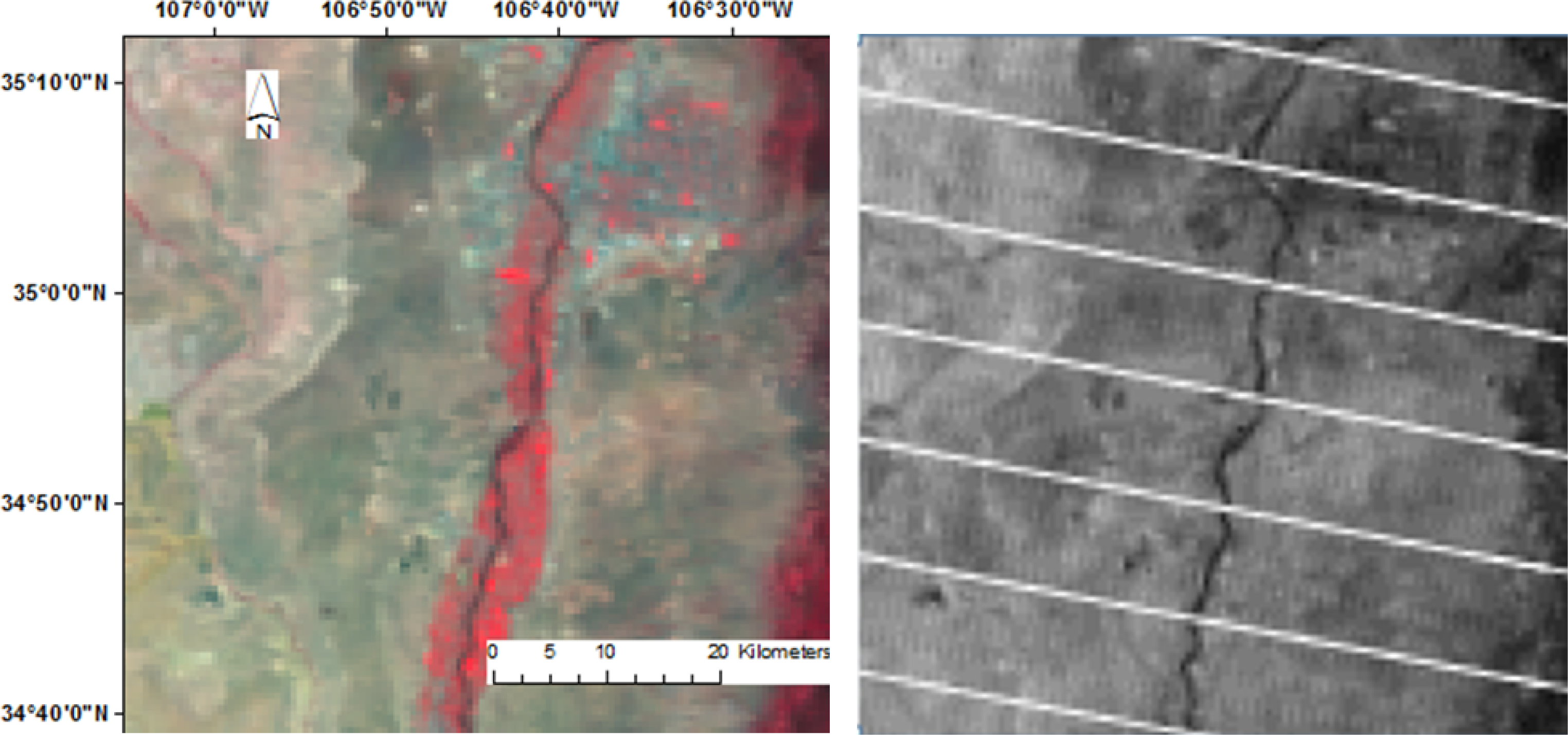
  • MOD02HKM. Calibrated radiances (MOD02) for band 1–7 at 500 m resolution (HKM = half kilometer). In this product, MODIS bands 1 and 2 are aggregated to 500 m from their nominal 250 m pixel size to coincide with bands 3–7. The product is used to produce radiances and reflectances for bands 1–7. The conversion of MOD02HKM digital numbers (DN) to at-satellite radiance values is performed using the following equation:
    L t , b = Rad s , b DN + Rad offs , b
    where Lt,b is at-satellite radiance in W/m2/sr/μm; Rads,b and Radoffs,b are the “radiance scales” and “radiance offsets” given for each band in the image metadata file. At-satellite reflectance is calculated using the following equation [16]:
    ρ t , b = π L t , b d r 2 ESUN b cos θ
    where Lt,b is at-satellite spectral radiance in band b (W/m2/sr/μm), and ESUNb is the mean solar exoatmospheric radiation over band b (W/m2/μm). Values of ESUNb for MODIS are included in Tasumi et al. [25]. Calculation of dr, cosθ follows procedures included in Allen et al. [16]. MOD02 is used to produce vegetation indices (NDVI, LAI), and surface albedo, which are utilized by several METRIC functions. Band 5 is commonly ignored due to systematic striping in this band.
  • MOD11_L2. Land surface temperature (LST). This image product represents surface temperature at satellite overpass time. LST is used in the computation of outgoing longwave solar radiation, and sensible heat (H) via the Tsvs. dT function of METRIC.
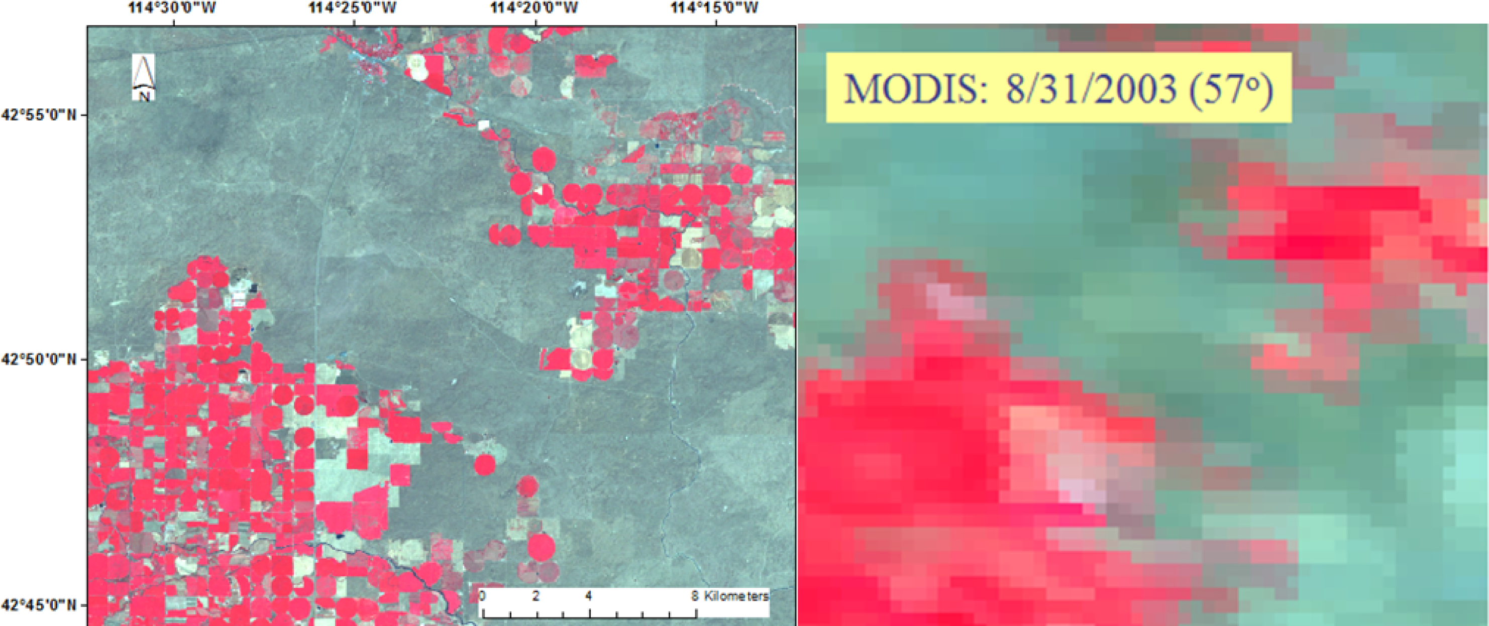
  • MOD03. Geolocation Fields. This file is needed to georegister the MOD02 and MOD11_L2 products. The file contains geodetic coordinates, solar zenith angle and sensor view angle for image overpass time. A maximum sensor view angle of less than 15°–20° is preferred in METRICM to avoid pixel deformation (bow tie effect) and fidelity loss (Figure 3). This is one reason why the 8- and 16-day products of MODIS are avoided with METRIC applications, because of difficulty in controlling the ingestion of information from days having large view angle.
  • MOD35. Cloud mask product. This is a useful product that helps to mask areas of clouds that are difficult to identify due to the coarse spatial resolution of MODIS.
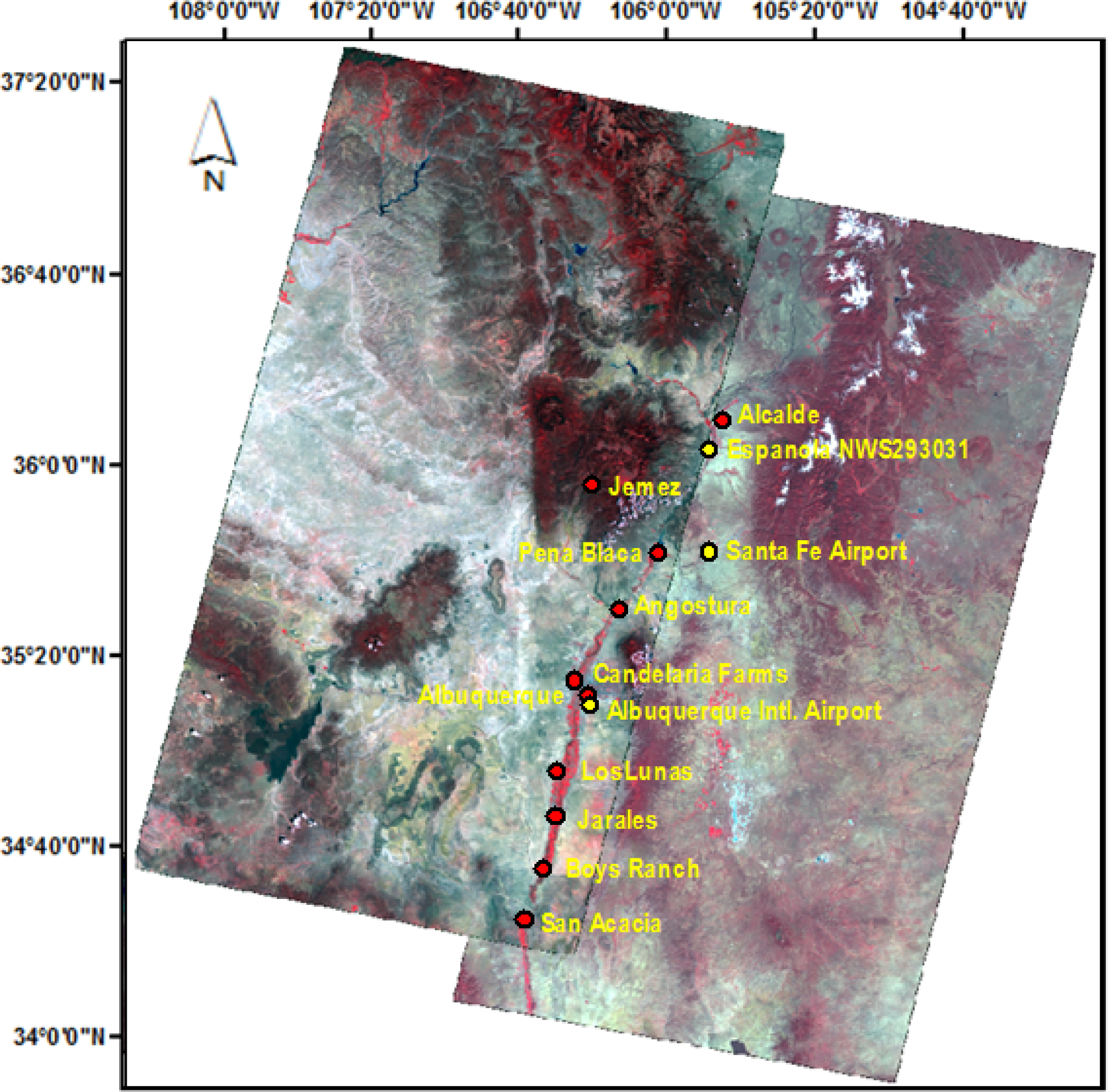
MODIS-Terra products were used in this paper. Equivalent MODIS-Aqua products can also be utilized for METRIC processing.

2.2. Study Area

The study area selected for illustration of a METRIC-MODIS application is the Middle Rio Grande region of northern and central New Mexico. METRICM was applied to a square area having the corner coordinates: 33°4′12″N to 36°22′10″N and 105°13′6″W to 108°9′59″W. The US Bureau of Reclamation (USBR) manages important irrigation and water conservation projects in this region. Surface water in the MRG comes from the natural flow of the Rio Grande basin and from supplemental sources provided by the San Juan-Chama and San Luis Valley Projects. Crop irrigation is the largest surface water use in the Basin, accounting for up to 90 percent of surface water withdrawals.

2.3. Application of METRIC to the Middle Rio Grande Using MODIS and Landsat

For comparison, the METRICL model [16] was applied to Landsat imagery for year 2002 for irrigated areas along the Middle Rio Grande valley from near Algodones south to near San Acacia. METRICM was applied to MODIS imagery for years 2002, 2005 and 2007 for the same region; these three years were requested by the USBR for its Evapotranspiration Toolbox system [34]. Thirteen Landsat and MODIS dates were processed for year 2002, spanning the period 14 January to 7 November, twenty one MODIS dates were processed for year 2005, spanning the period 6 January to 24 December, and twenty six MODIS dates were processed for year 2007, spanning the period 28 January to 30 December. Eleven of the thirteen MODIS image dates in 2002 are the same dates as those processed using Landsat 7 imagery to provide opportunity for cross-comparisons, as shown in Table 3.
All MODIS image dates were selected to limit satellite sensor view angles to less than about 15° for the areas of interest, along with cloud free conditions for the MRG area. The following sections briefly describe the calibration of METRICM, which was performed uniquely for each image date. The calibration process for METRIC is detailed in Allen et al. [16] and involves the selection of ‘hot’ and ‘cold’ pixels and conditions where the sensible heat flux components of the energy balance are calibrated, as mentioned in previous sections.

2.3.1. Specific MODIS Products Used for the MRG Application

At the time of processing, MODIS radiances, geolocation fields, and cloud mask products were obtained from the NASA Level 1 and Atmosphere Archive and Distribution System (LAADS) website. Land surface temperature (LST) version 5, used for 2005 and 2007, was obtained from the Earth Observing System Gateway. Version 4 LST was used for 2002.

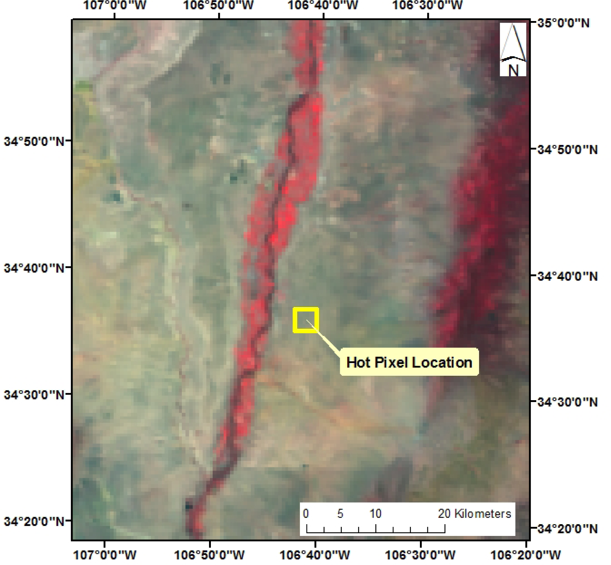
2.3.2. Hot Pixel Selection

As previously noted, with MODIS imagery, where thermal pixels have a spatial resolution of 1,000 m, it is difficult to identify a 1 km2 agricultural bare-soil area that has uniform conditions. This can become even more of a problem when attempting to identify a pixel having relatively consistent uniformity over time. Spatial uniformity over time facilitates the automation of the calibration procedure by using the same location each image date for the hot pixel. In the New Mexico application a 2.5 km by 2.5 km dry, flat desert area SE of Albuquerque was selected to routinely serve as the hot pixel, as shown in Figure 4. This location had relatively uniform, sparse vegetation in space and time and represented a condition where ET for each image date could be estimated from a precipitation-based water balance. This same location was used for all three years of application and was selected based on results from a Landsat-based application of METRIC for 2002 [22]. Evaporation was assumed to be ∼0 for this location for periods having little or no recent antecedent precipitation, and was set to a positive value for some dates based on a daily surface soil water balance driven by weather data and precipitation data from Middle Rio Grande Conservation District (MRGCD) automated weather stations, as described in a following section. All parameters used in the energy balance of the hot pixel condition during METRIC calibration, for example, albedo and surface roughness, were averaged over the 2.5 km by 2.5 km area.

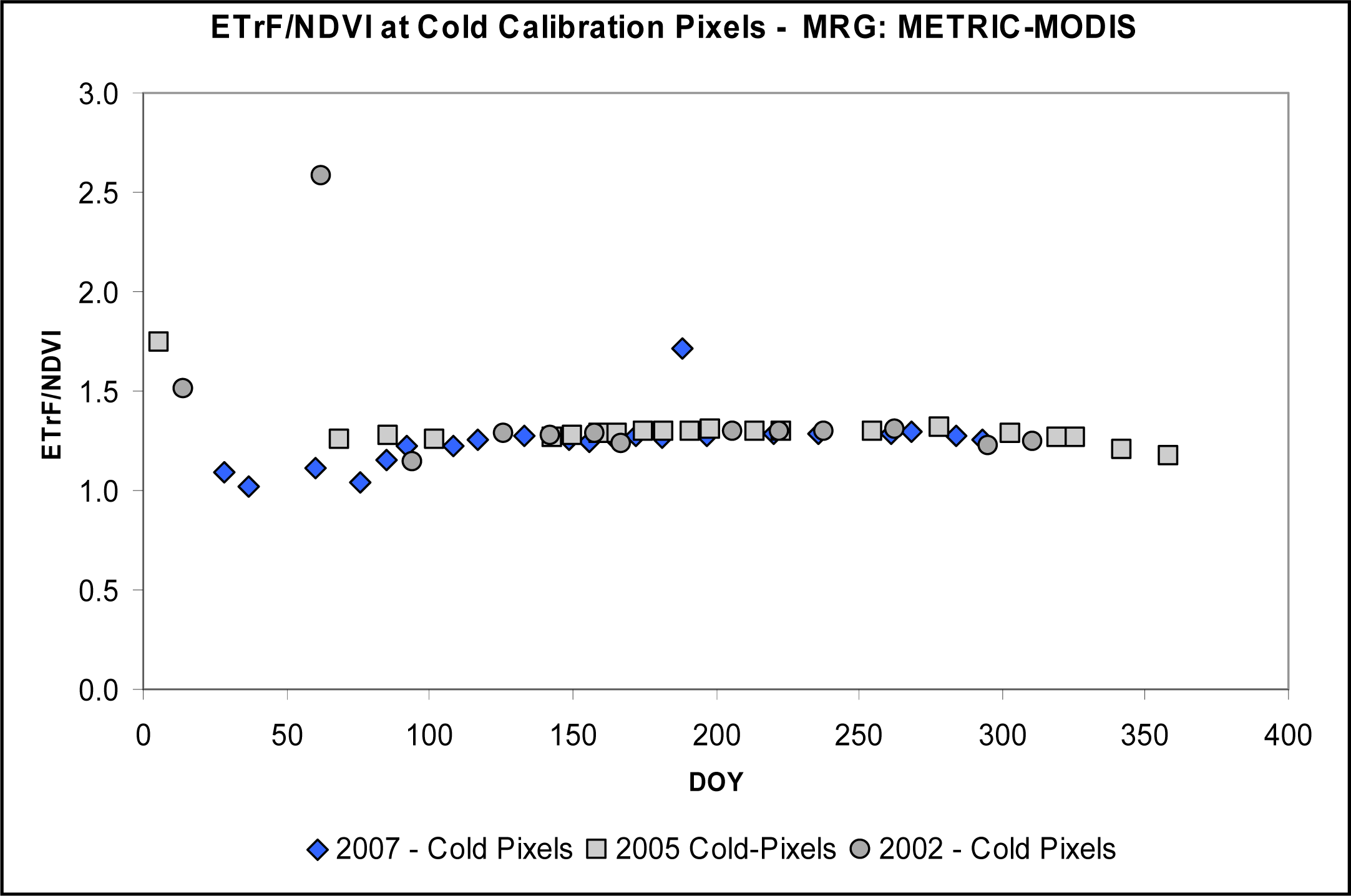
2.3.3. Cold Pixel Selection

The cold calibration pixel of METRIC, when applied with Landsat imagery, is identified as a fully vegetated pixel having a low surface temperature and where the assumption that its ET is approximately equal to 1.05× alfalfa reference ETr is assumed to hold [16,17]. These types of pixels are relatively easy to identify with Landsat imagery where the 30 m resolution for short wave reflectance and 60 to 120 m resolution for surface temperature causes many pixels to lie within individual fields. With MODIS, where resolution for short wave is 500 m and for thermal is 1,000 m, it is nearly impossible to find a single pixel having uniform, full vegetation cover and maximum ET, since 1,000 m pixels nearly always span multiple agricultural fields or clusters of other vegetation types. This is especially true in the Middle Rio Grande valley where agricultural and riparian areas lie within a relatively thin river corridor and farm sizes are characteristically small. Therefore, alternative methods were explored for calibrating METRIC to MODIS images for the “cold pixel” condition.
Two methods were tested for identifying the cold pixel condition and assigning an ETrF value. (1) Determination of the ETrF value to assign to the ‘cold’ pixel based on the normalized difference vegetation index (NDVI) of one or more pixels having the cooler temperatures in the image, and (2) using the ‘SEBAL approach’ of Bastiaanssen et al. [10,11], where one assumes that the skin temperature of a local water body is at the temperature at which the sensible heat flux, H, to the air becomes zero or nearly zero.2.3.4. Assignment of ETrF value for the cold pixel
Tasumi et al. [22] developed an ETrF vs. NDVI relationship for the MRG area by aggregating METRIC-derived ETrF from 30 m resolution Landsat images (METRICL) into MODIS scale data. The METRICL-based ETrF products were degraded to 1 km and values were correlated with MODIS-based NDVI computed from at-surface reflectances, producing a MODIS-scale ETrF vs. NDVI function. The resulting relationship used in this study to estimate the ETrF associated with the higher end of NDVI values in the image is:
ETrF cold = 1.51 NDVI cold 0.145
where the NDVI is based on MODIS-derived surface reflectance. Three different procedures were used to identify and quantify the NDVI for groups of pixels to be associated with the cold pixel (NDVIcold) for application of Equation (18). These procedures evolved each time a new year was processed.
Procedure 1: applied to Year 2002. The ETrF -NDVI relationship of Equation (18) was applied to the average NDVI of five 500 m sized pixels in a 260 km tall × approximately 5 km wide, mostly agricultural corridor lying along the Rio Grande between Alcalde and San Acacia for each MODIS image date, where the five pixels had the highest NDVI values. Landsat images were used to assist in the process of identifying pixels lying within agricultural areas. The resulting average NDVI was inserted into Equation (18) to estimate ETrF that was then assigned to the cold pixel condition of METRIC. One of the five pixels that had surface temperature close to the mean surface temperature of the five pixels was assigned as the cold pixel, for purposes of estimating albedo, aerodynamic roughness, etc. in the energy balance of the cold pixel condition.
Procedure 2: applied to Year 2005. For 2005, the ETrF -NDVI relationship was applied to the average NDVI of the twenty 500 m pixels in the same region of interest having the highest NDVI values. The mean NDVI of those 20 pixels was applied with Equation (18) to estimate the ETrF associated with the cold pixel condition. Equation (18) was applied to all images. The ETrF average assigned to the ‘cold’ pixel condition ranged from about 0.8 to 0.9 during the growing season, indicating a 15 to 25% reduction in ET relative to ET normally assigned to a fully vegetated, fully watered condition during application with Landsat [16]. This decrease was due to the absence of complete, 1,000 m MODIS thermal pixels that had full (dense and green) vegetation cover.
Procedure 3: applied to Year 2007. For 2007, the cold pixel selection was assisted by the statistical method of Allen et al. [29] similar to that described earlier for automated calibration of METRIC for Landsat images. In the application to year 2007 MODIS images, the sub-population of pixels within the agricultural corridor of the MRG system that contained the 10% highest values for NDVI were isolated. From within that population, we selected the pixels having the lower 20% of surface temperatures. This resulted in 2%, or 96, of the total 4,800 500-m pixels lying within the corridor being retained for the cold pixel assessment and assignment. As an independent check, the procedure of 2005 was also applied, where NDVI was averaged for the twenty 500 m pixels in the MODIS image having the highest NDVI values. In both cases, the mean NDVI for the selected pixels was used with the ETrF-NDVI relationship of Equation (18) to estimate the ETrF to be associated with the cold pixel condition, and one pixel of the subpopulation having surface temperature close to the mean surface temperature of the subpopulation was then assigned as the cold pixel, with albedo, NDVI, and other estimates for that pixel used for the energy balance of the cold pixel condition.

2.3.5. Reference ET

Reference ET is used in METRIC for calibration of the sensible heat flux function, for application of a daily soil evaporation process model to assign any residual evaporation on the image date to the hot pixel, and to aggregate ET between satellite overpass dates by multiplying ETrF interpolated for each day between images by the daily ETr value. In this study, ETr was calculated on an hourly timestep employing the 2005 ASCE-EWRI standardized Penman-Monteith method [24] for the 0.5 m tall alfalfa reference crop basis, using data from automated weather stations operated by the Middle Rio Grande Conservancy District (MRGCD). Two weather stations, Angostura and Jarales, were utilized due to their completeness of record, quality of data, and locations in agricultural settings within the corridor, necessary to produce accurate and representative ETr for irrigated conditions [24]. A strict quality control analysis based on ASCE-EWRI [24] was applied to all weather data and corrections or adjustments to data were made. Hourly ETr was used in the calibration of METRIC to each satellite image date and was summed to 24-h totals during creation of daily, monthly and annual ET imagery. Locations of the Angostura and Jarales MRGCD stations are shown in Figure 5. The ETr from the two stations was averaged prior to use in image calibration.

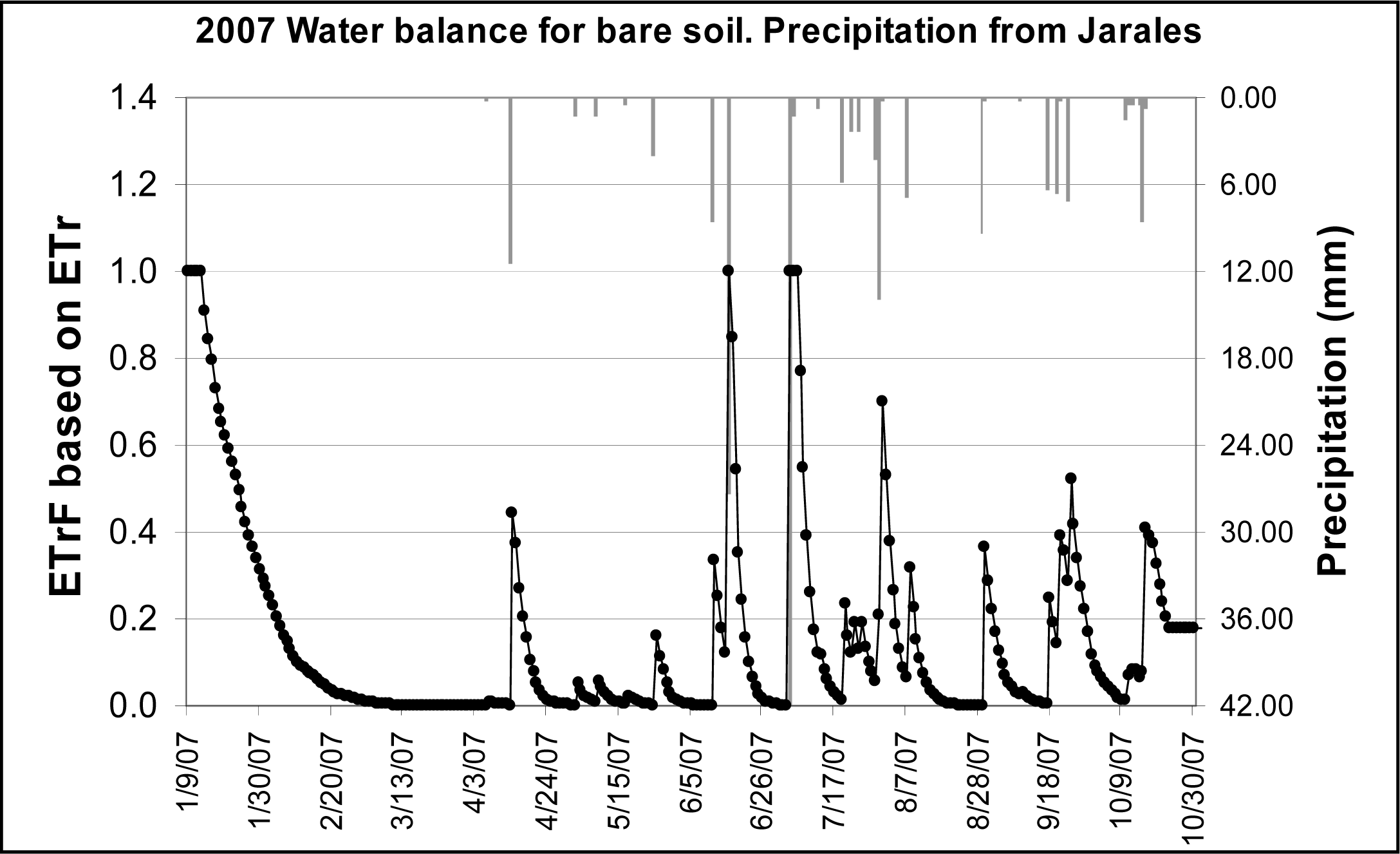
2.3.6. Water Balance for the Hot Pixel

The soil water balance used to estimate the soil water content and to assign any residual evaporation to the hot pixel on the image dates was based on the FAO-56 procedure [23]. Precipitation data were taken from the Jarales weather station because of its proximity to the hot pixel location. Evaporation estimated from the daily soil water balance, expressed as ETrF, and daily precipitation are shown in Figure 6 for 2007.

3. Results

3.1. Evaluation of Consistency in Calibration Pixel Selection

As described previously, a somewhat different procedure was used each year to select or assign the cold pixel condition for METRIC calibration as part of evolving a preferred technique. In all three years, the maximum ETrF average assigned to the cold pixel condition ranged from about 0.8 to 0.9, depending on the mean value of NDVI, indicating a 15 to 25% reduction in ET relative to ET expected for a fully vegetated, fully watered condition. The application of two methods for selecting a cold pixel for year 2007 generally resulted in different values for NDVI and Ts, but with similar METRIC calibration due to the symbiotic relationship between ET and Ts in the surface energy balance. Values for mean NDVI and assigned ETrF for the 96 pixels filtered as the coolest, most vegetated 2%, tended to run somewhat lower than the mean NDVI and assigned ETrF for the 20 pixels having the highest NDVI; however, the Ts associated with the mean NDVI of the 96 pixels tended to run somewhat higher than that for the 20 pixels. This outcome suggests that the selection of the cold pixel condition for an image and magnitude of ETrFcold is not critical so long as the ETrFcold, NDVI, Ts and albedo all correspond to the same equilibrium energy balance condition. The final calibration and production of an accurate ET image does require that Equation (18) be locally calibrated or verified using Landsat-based applications or other methods.
Because Equation (18) was used to calculate the ETrFcold associated with the NDVI for the cold pixel condition each year, the ratio between ETrF and NDVI remained steady among years as shown in Figure 7. ETrF/NDVI > 1.5 for image dates having antecedent rainfall where special adjustments to ETrFcold was made to account for the extra wetness. The ETrF/NDVI for the hot pixel calibration changed substantially with image and year due to effects of antecedent soil moisture. The statistical approach used for year 2007 has the desirable attribute of being nearly automatable and it is recommended for applications of METRIC with MODIS imagery.

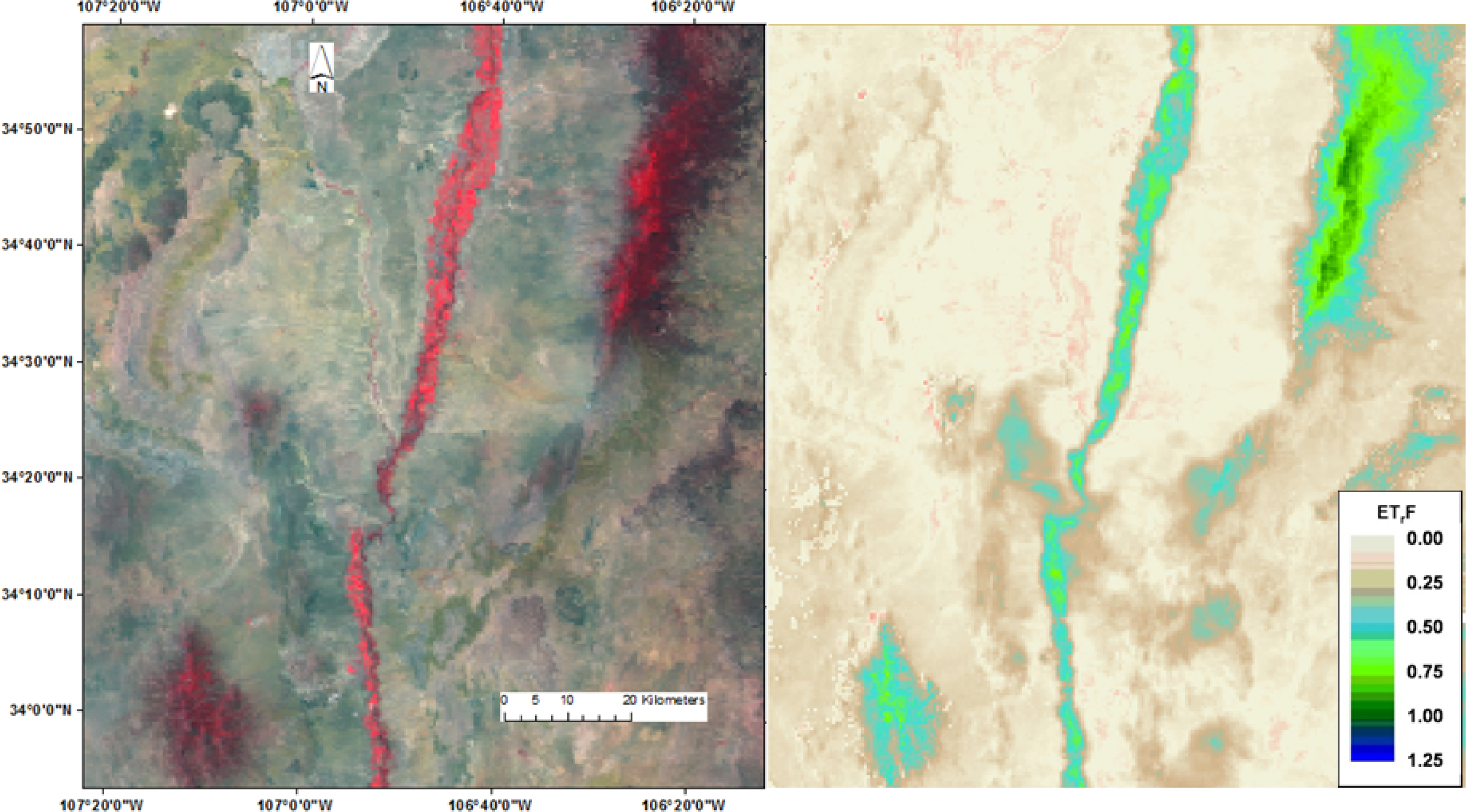
3.2. Results from METRICM application

METRIC-MODIS (METRICM) was applied using the unique calibration of each image via the hot and cold pixel selection and assignment of ETrF values. In some desert areas, where surface temperature was sometimes much hotter than at the hot pixel temperature due to apparently low soil heat flux rates and shielding of the soil surface by dry brush, the slope of the Ts for dT function was reduced by a factor of 4, when Ts exceeded the hot pixel temperature to place upper bounds on H. In addition, soil heat flux (G) estimates were reduced during this occurrence as detailed by Allen et al. [16]. Actual G was speculated to be lower for the dry, hot desert soils because of reduced thermal conductance caused by crusting, dryness and delamination of upper soil layers and lower density and associated particle to particle contact [16].
The Rio Grande corridor was clear in most of images, which facilitated interpolation of daily to monthly and seasonal ET following procedures and assumptions detailed in Allen et al. [16]. An example of a daily ET map is shown in Figure 8 for 06/30/2007.
ETrF for a 500 m MODIS pixel located in a typical agricultural area as shown on Figure 9 is plotted in Figure 10 to illustrate the evolution of ETrF during 2007. Variation of ETrF with DOY reflects the different crop stages during the growing season. The three gray points in Figure 10 have high values for ETrF due to significant precipitation events.
Figure 11 shows the variation of ETrF for a desert area from January to September 2007. Negative values for ETrF reflect the uncertainties in the estimation of near-zero ET as a residual in the surface energy balance. The negative values essentially represent variance about the nearly zero ET mean. ETrF rose above about 0.10 during July and August, reflecting ET and vegetation growth stimulated by the summer monsoon.

3.3. Comparison between Landsat and MODIS sApplications for Year 2002

ET images produced by the METRICM application were compared with those produced by the METRIC-LANDSAT (METRICL) application for year 2002. In Figure 12, METRICM ETrF results, averaged over major portions of the MRG valley from near Algodones south to near San Acacia, were close to those for METRICL(R2 = 0.899; RMSE = 0.037). Annual estimated ET over the valley for year 2002 was 1,045 mm from the METRICM application and 1,067 mm from the METRICL application. The difference was 2%. Other investigators have also reported close agreement between ET maps generated using SEBAL with MODIS and using SEBAL with Landsat images in the Middle Rio Grande Valley [32] and in the White Volta Basin [33].
ET produced by the METRICM method performed better, relative to the METRICL application, than did a test application using the classical SEBAL calibration method with MODIS images, where, in the classical method, the temperature for the ‘cold’ pixel condition is taken as water temperature, which in this case was represented by the temperature of Elephant Butte Reservoir. In the SEBAL method, sensible heat flux (H) is assumed to be zero for the water surface temperature, whereas, in the METRIC method, hourly alfalfa reference ETr is used to calibrate the energy balance process for the cold condition. The ‘hot pixel’ selection for calibrating METRIC and SEBAL were the same. The MODIS-SEBAL approach for the cold pixel calibration tended to underestimate ETrF for the six dates processed (Figure 12).

3.4. Comparisons for Specific Locations

Figure 13 shows Landsat and MODIS based ETrF for selected areas having high NDVI and low NDVI, analyzed by sampling over 2 km areas. The graph provides an idea of general values for the ETrF near the cold/hot pixel selections. At locations having relatively high NDVI, MODIS ETrF was close to that from Landsat. Figure 13 shows MODIS ETrF was underestimated for image no. 9 (8/10/2002). Otherwise, comparisons were quite good. Agreement was also very good for the locations having low NDVI. ETrF was high for the first two images due to antecedent rainfall.

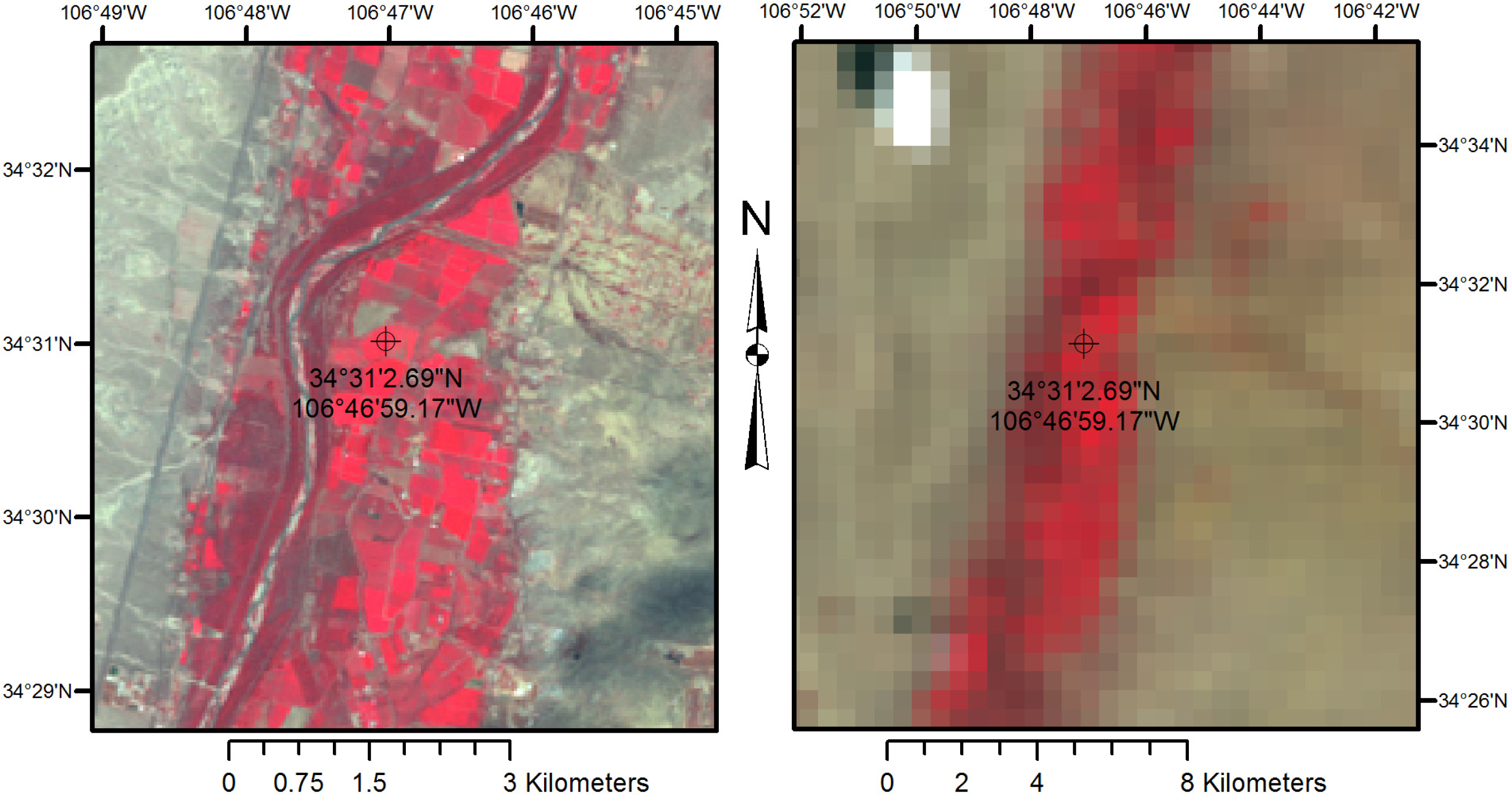
3.5. Impact of MODIS Resolution

Figure 14 is similar to Figure 13, but where the analysis was conducted by sampling 500 m pixels, rather than aggregation to 2 km sized areas. At the 500 m scale, METRICM consistently underestimated ETrF at high-NDVI locations relative to METRICL because the MODIS thermal band has 1 km resolution that is compromised by pixels neighboring a specific 500 m pixel.
Good agreement between METRICM and METRICL was found for low-NDVI locations at the 500 m scale. This was most likely due to the presence of relatively large clusters of 500 m pixels having similar vegetation and land cover and surface temperature, so that the surface temperature value was not compromised by different surface temperatures of neighboring pixels.

3.6. Calculation of Monthly and Seasonal ET

Integration of ET over time is typically done in METRIC by interpolating ETrF in between available processed image dates using spline or other interpolation technique to create a daily time series of ETrF for each pixel. The result is very similar to the construction of a continuous ‘crop coefficient’ curve. The daily interpolated ETrF is multiplied by daily ETr computed from daily or hourly weather data to capture the day to day impacts of weather on ET, even under clouded conditions. When time intervals between images are greater than about 20 days, it is preferable and likely more accurate to use a spline function for interpolation, rather than linear interpolation, to better approximate the general shape of vegetation development curves. Generally, one satellite image per month is sufficient to construct an accurate ETrF curve for purposes of estimating seasonal ET. Allen et al. [17] described the tendency of random error in ETrF on individual overpass dates to partially self-cancel when extended over multiple overpass dates, similar to the reduction in the standard deviation of a mean value with increasing degrees of freedom. In this work, a linear interpolation of ETrF values was performed due to the availability of frequent cloud-free images in the MRG area for the processed years.

3.7. Aggregation to the ET-Toolbox Grid

The monthly ET produced from MODIS was aggregated into 4 km sized grid cells of the ET-Toolbox grid managed by the US Bureau of Reclamation and MRGCD as part of their river management program [34]. An example of maps of monthly ET along the MRG computed by interpolating between satellite image dates is shown in Figure 15. Data in these maps compared favorably with estimates of ET by the ET-Toolbox method as reported by Allen et al. [35] and Hendrickx et al. [36] but showed better spatial variability due to the use of surface energy balance. ET maps generated from surface energy balance models like METRIC can provide useful data to develop or test more simplistic approaches like the use of vegetation indices to retrieve crop coefficients from MODIS [37].

3.8. Uncertainty of ET Estimates

Trusted ground-based measurements of actual ET were not available for the study area to compare with the METRIC applications from MODIS and Landsat. However, comparisons of METRIC-based products with actual ET estimated by the ET-Toolbox system, as noted in Section 3.7, did indicate similar results. The higher spatial resolution of Landsat, where the 30 m size of short-wave pixels and 60 to 120 m of long-wave pixels for Landsat 7 and Landsat 5, respectively, provides the opportunity to sample spectral information originating from individual fields for field sizes greater than about 4 ha. In contrast, the 500 to 1,000 m size of MODIS pixels limits the size of field that can be sampled apart from influence of adjacent fields to about 200 to 400 ha. Because the typical size of agricultural fields along the Middle Rio Grande valley ranges from 2 to 40 ha, only Landsat-based ET mapping can provide a high level of certainty regarding the actual ET associated with any one field. Uncertainty of MODIS-based estimates would be substantial for individual fields surrounded by other fields or land-uses having substantially different amounts of vegetation, water supply, or irrigation practices. However, when aggregated over larger areas, such as the 4 km sized grid cells of the ET-Toolbox system or larger irrigated regions of the valley, Landsat- and MODIS-based applications of METRIC produce similar results and therefore have similar levels of uncertainty at the larger spatial levels.

4. Conclusions

The METRIC energy balance model was applied using MODIS data along the Middle Rio Grande of New Mexico to estimate actual evapotranspiration for years 2002, 2005, and 2007. METRIC was also applied using Landsat imagery for year 2002. This provided the opportunity to use Landsat-based ET to develop a calibration scheme to use with MODIS imagery and to compare METRIC-MODIS results with those from METRIC-Landsat. The application of METRIC with MODIS is challenging due to some quality issues associated with MODIS products and the coarse grid size of thermal data (1 km). The main challenge with the application with MODIS is the selection of cold and hot pixels used in METRIC calibration, due to the spatial resolution of MODIS thermal and shortwave pixels. The solution to calibration with MODIS imagery was to assign an ETrF value to the identified cold pixel condition based on an ETrF vs. NDVI relationship developed using METRIC-Landsat-ETrF degraded to MODIS spatial resolution. For the hot pixel, a fixed area located in a desert location was used and its ETrF value was assigned based on a soil water balance performed using local precipitation and soil conditions. The training of the calibration scheme using Landsat-based ET enabled METRIC-MODIS ETrF results, averaged over major portions of the Middle Rio Grande valley, to agree closely with those from METRIC-LANDSAT (R2 = 0.899; RMSE = 0.037). Annual estimated ET averaged over the valley for year 2002 was 1,045 mm from the METRIC-MODIS application and 1,067 mm from the METRIC-Landsat application. This same calibration approach should be applicable in other regions, where the ‘close-up’ analyses by Landsat provide a sound basis for informing MODIS-based calibrations regarding relative ET rates associated with specific locations and vegetation amounts.

Acknowledgments

The writers acknowledge NASA-ROSES and USDA-CSREES that provided funding support plus cooperation by the US Bureau of Reclamation. They also acknowledge the technical and scientific contributions provided by Jan Hendrickx of New Mexico Tech, Magali Garcia of the Universidad Mayor de San Andres in Bolivia, and Clarence Robison and Carlos Kelly of the Kimberly Research and Extension Center of the University of Idaho.

Conflict of Interest

The authors declare no conflict of interest.

References

  1. Kustas, W.P.; Norman, J.M. Use of remote sensing for evapotranspiration monitoring over land surfaces. Hydrol. Sci. J 1996, 41, 495–515. [Google Scholar]
  2. Bastiaanssen, W.G.M. Remote Sensing in Water Resources Management: The State of the Art; IWMI: Sri Lanka, 1998. [Google Scholar]
  3. Courault, D.; Seguin, B.; Olioso, A. Review on estimation of evapotranspiration from remote sensing data: from empirical to numerical approaches. Irrig. Drain. Syst 2005, 19, 223–249. [Google Scholar]
  4. Kalma, J.D.; McVicar, T.R.; McCabe, M.F. Estimating land surface evaporation: A review of methods using remotely sensed surface temperature data. Surv. Geophys 2008, 29, 421–469. [Google Scholar]
  5. Anderson, M.; Allen, R.G.; Morse, A.; Kustas, W.P. Use of Landsat thermal imagery in monitoring evapotranspiration and managing water resources. Remote Sens. Environ 2012, 122, 50–65. [Google Scholar]
  6. Crow, W.T.; Kustas, W.P.; Prueger, J.H. Monitoring root-zone soil moisture through the assimilation of a thermal remote sensing-based soil moisture proxy into a water balance model. Remote Sens. Environ 2008, 112, 1268–1281. [Google Scholar]
  7. Nagler, P.; Glenn, E.; Nguyen, U.; Scott, R.; Doody, T. Estimating riparian and agricultural actual evapotranspiration by reference evapotranspiration and MODIS enhanced vegetation index. Remote Sens 2013, 5, 3849–3871. [Google Scholar]
  8. Tang, R.; Zhao-Liang, L.; Tang, B. An application of the Ts-VI triangle method with enhanced edges determination for evapotranspiration estimation from MODIS data in arid and semi-arid regions. Remote Sens. Environ 2010, 114, 540–551. [Google Scholar]
  9. Yang, Y.; Shang, S.; Jiang, L. Remote sensing temporal and spatial patterns of evapotranspiration and the responses to water management in a large irrigation district of North China. Agric. For. Meteorol 2012, 164, 112–122. [Google Scholar]
  10. Bastiaanssen, W.G.M.; Menenti, M.; Feddes, R.A.; Holtslag, A.A.M. A remote sensing surface energy balance algorithm for land (SEBAL): 1. Formulation. J. Hydrol. 1998, 212–213, 198–212. [Google Scholar]
  11. Bastiaanssen, W.G.M.; Pelgrum, H.; Wang, J.; Ma, Y.; Moreno, J.; Roerink, G.J.; van der Wal, T. The Surface Energy Balance Algorithm for Land (SEBAL): Part 2 validation. J. Hydrol 1998, 212–213, 213–229. [Google Scholar]
  12. Bastiaanssen, W.G.M. Regionalization of Surface Flux Densities and Moisture Indicators in Composite Terrain: A Remote Sensing Approach under Clear Skies in Mediterranean Climates. 1995; p. 273. [Google Scholar]
  13. Ruhoff, A.; Paz, A.; Collischonn, W.; Aragao, L.; Rocha, H.; Malhi, Y. A MODIS-based energy balance to estimate evapotranspiration for clear-sky days in Brazilian tropical savannas. Remote Sens 2012, 4, 703–725. [Google Scholar]
  14. Jia, L.; Xi, G.; Liu, S.; Huang, C.; Yan, Y.; Liu, G. Regional estimation of daily to annual regional evapotranspiration with MODIS in the Yellow River delta wetland. Hydrol. Earth Syst. Sci 2009, 13, 1775–1787. [Google Scholar]
  15. Mu, Q.; Zhao, S.; Running, S. Improvements to a MODIS global terrestrial evapotranspiration algorithm. Remote Sens. Environ 2011, 155, 1781–1800. [Google Scholar]
  16. Allen, R.G.; Tasumi, M.; Trezza, R. Satellite-based energy balance for mapping evapotranspiration with internalized calibration (METRIC)—Model. ASCE J. Irrig. Drain. Eng 2007, 33, 380–394. [Google Scholar]
  17. Allen, R.G.; Tasumi, M.; Morse, A.; Trezza, R.; Kramber, W.; Lorite, I.; Robison, C.W. Satellite-based energy balance for mapping evapotranspiration with internalized calibration (METRIC)—Applications. ASCE J. Irrig. Drain. Eng 2007, 133, 395–406. [Google Scholar]
  18. Allen, R.G.; Tasumi, M.; Morse, A.; Trezza, R. A Landsat-based energy balance and evapotranspiration model in Western US water rights regulation and planning. J. Irrig. Drain. Syst 2005, 19, 251–268. [Google Scholar]
  19. Tasumi, M.; Trezza, R.; Allen, R.G.; Wright, J.L. Operational aspects of satellite-based energy balance models for irrigated crops in the semi-arid U.S. J. Irrig. Drain. Syst 2005, 19, 355–376. [Google Scholar]
  20. Tasumi, M.; Allen, R.G.; Trezza, R.; Wright, J.L. Satellite-based energy balance to assess within-population variance of crop coefficient curves. ASCE J. Irrig. Drain. Eng 2005, 131, 94–109. [Google Scholar]
  21. Allen, R.G.; Tasumi, M.; Trezza, R. Benefits from Tying Satellite-Based Energy Balance to Reference Evapotranspiration. In Earth Observation for Vegetation Monitoring and Water Management: Naples, Italy, 10–11 November 2005; D’Urso, G., Jochum, A., Moreno, J., Eds.; American Institute of Physics: College Park, MD, USA, 2005; pp. 127–137. [Google Scholar]
  22. Tasumi, M.; Trezza, R.; Allen, R.G. METRIC Manual for MODIS Image Processing Version 1.0 (April, 2006); University of Idaho R&E Center: Kimberly, IA, USA, 2006; p. 67. [Google Scholar]
  23. Allen, R.G.; Pereira, L.S.; Raes, D.; Smith, M. Crop Evapotranspiration: Guidelines for Computing Crop Water Requirements; Irrigation and Drainage Paper 56; United Nations FAO: Rome, Italy, 1998; p. 300. [Google Scholar]
  24. ASCE-EWRI. The ASCE Standardized Reference Evapotranspiration Equation; ASCE-EWRI Standardization of Reference Evapotranspiration Task Committee Report; ASCE: Reston, VA, USA, 2005; p. 216. [Google Scholar]
  25. Tasumi, M.; Allen, R.; Trezza, R. At-surface albedo from Landsat and MODIS satellites for use in energy balance studies of evapotranspiration. J. Hydrol. Eng 2008, 13, 51–63. [Google Scholar]
  26. Starks, P.J.; Norman, J.M.; Blad, B.L.; Walter-Shea, E.A.; Walthall, C.L. Estimation of shortwave hemispherical reflectance (albedo) from bidirectionally reflected radiance data. Remote Sens. Environ 1991, 38, 123–134. [Google Scholar]
  27. MODIS UCSB Emissivity Library. 2012. Available online: http://www.icess.ucsb.edu/modis/EMIS/html/em.html (accessed on 15 March 2012).
  28. Myneni, R.; Knyazikhin, Y; Zhang, Y.; Tian, Y.; Wang, Y.; Privette, J.; Morisette, J.; Running, S.; Nemani, R. MODIS Leaf Area Index (LAI) and Fraction of Photosynthetically Active Radiation Absorved by Vegetation (FPAR) Product (MOD15) Algorithm Theoretical Basis Document. Version 4.0; 1999. Available online: http://modis.gsfc.nasa.gov/data/atbd/atbd_mod15.pdf (accessed on 1 April 2008).
  29. Allen, R.G; Burnett, B.; Kramber, W.; Huntington, J.; Kjasersgaard, J.; Kilic, A.; Kelly, C.; Trezza, R. Automated calibration of the METRIC-Landsat evapotranspiration process. J. Am. Water Resour. Assoc 2013, 49, 563–576. [Google Scholar]
  30. Allen, R.G. Skin layer evaporation to account for small precipitation events—An enhancement to the FAO-56 evaporation model. Agric. Water Manage 2011, 99, 8–18. [Google Scholar]
  31. NASA Earth Observing System Data and Information System (EOSDIS); 2012. http://reverb.echo.nasa.gov/reverb (accessed on 15 January 2013).
  32. Hong, S.-H.; Hendrickx, J.M.H.; Borchers, B. Effect of scaling transfer between evapotranspiration maps derived from LandSat 7 and MODIS images. Proc. SPIE 2005, 5811, 147–158. [Google Scholar]
  33. Compaoré, H.; Hendrickx, J.M.H.; Hong, S.-H.; Friesen, J.; van de Giesen, N.C.; Rodgers, C.; Szarzynski, J.; Vlek, P.L.G. Evaporation mapping at two scales using optical imagery in the White Volta Basin, Upper East Ghana. Phys. Chem. Earth, Parts A/B/C 2008, 33, 127–140. [Google Scholar]
  34. US Bureau of Reclamation. ET Toolbox, Evapotranspiration Toolbox for the Middle Rio Grande. A Water Resources Decision Tool. 2008. Available online: http://www.usbr.gov/pmts/rivers/awards/ettoolbox.pdf (accessed on 15 January 2013).
  35. Allen, R.G.; Tasumi, M.; Robison, C.; Trezza, R.; Garcia, M. Exploration of ET Coefficients Derived Using MODIS Satellite-Based METRIC ETrF vs. Awards/ET-Toolbox Based ET Coefficients within the Middle Rio Grande Valley; University of Idaho Report; University of Idaho: Kimberly, IA, USA, 2008; p. 37. [Google Scholar]
  36. Hendrickx, J.; Allen, R.; Brower, A.; Byrd, A.; Hong, S.; Ogden, F.; Pradhan, N.; Robison, C.; Toll, D.; Trezza, R.; Umstot, T; Wilson, J. Benchmarking optical/thermal satellite imagery for estimation of evapotranspiration and soil moisture in decision support tools. J. Am. Water Resour. Assoc, 2013; submitted. [Google Scholar]
  37. Kamble, B.; Kilic, A.; Hubbard, K. Estimating crop coefficients using remote sensing-based vegetation index. Remote Sens 2013, 5, 1588–1602. [Google Scholar]
Figure 1. (Left) MODIS-Terra image (combination 2,1,4) for 05/29/2007 near Albuquerque, NM. (Right) MODIS band 5 corresponding to the same image showing stripes.
Remotesensing 05 05397f1
Figure 2. At-surface NDVI vs. LAI for six surfaces (MODIS backup method), and generalized curve (METRIC LAI).
Remotesensing 05 05397f2
Figure 3. (Left) Landsat image (combination 4,3,2) for 08/31/2003 near Minidoka, southern Idaho. (Right) MODIS-Terra image (2,1,4) for the same day, taken at 57° sensor view angle, showing substantial pixel deformation and smearing.
Remotesensing 05 05397f3
Figure 4. Hot pixel location used to calibrate METRIC for all MODIS images.
Remotesensing 05 05397f4
Figure 5. “False color” Landsat images for WRS-2 Paths 33 and 34, rows 34–36, of Landsat showing locations of weather stations along the Middle Rio Grande. Vegetated areas along the MRG river corridor are displayed as the bright red vertical strip in the image center. This area approximates the one processed using MODIS imagery.
Remotesensing 05 05397f5
Figure 6. Evaporation estimated using a daily soil water balance for a bare soil condition based on reference ET and precipitation data from Jarales, 2007. Daily precipitation is shown on the right y-axis and is plotted from the top of the figure.
Remotesensing 05 05397f6
Figure 7. Comparison of ETrF/NDVI for the cold pixel calibration condition for application of METRICM to the MRG region during years 2002, 2005 and 2007.
Remotesensing 05 05397f7
Figure 8. (Left) false color MODIS image for 06/30/2007 (2,1,4 combination). (Right) corresponding ETrF map.
Remotesensing 05 05397f8
Figure 9. Location of an agricultural pixel (circular cross-hair) used to plot ETrF evolution in Figure 10. (Left) Landsat 5 image used as a reference (08/16/2007). (Right) MODIS image (08/24/2007).
Remotesensing 05 05397f9
Figure 10. Variation of ETrF, obtained from METRIC, from January to September 2007 (black symbols). High values of ETrF following recent precipitation events are shown in gray color. The solid black line shows the general tendency of the ETrF data.
Remotesensing 05 05397f10
Figure 11. Variation of ETrF, obtained from METRIC, from January to September 2007, obtained by averaging several pixels in a desert area.
Remotesensing 05 05397f11
Figure 12. Average ETrF for the MRG valley, calculated by METRICM, METRICL and MODIS-SEBAL for 12 images during 2002. Image no. 13 was not included due to many small clouds over MRG. The ETrF is based on the ASCE-EWRI [24] standardized Penman-Monteith alfalfa reference equation.
Remotesensing 05 05397f12
Figure 13. MODIS and Landsat based average ETrF for locations having high vegetation (NDVI = 0.50 or higher) and low vegetation (NDVI = 0.20 and lower) along the Middle Rio Grande valley corridor during 2002, sampled with 2 km resolution.
Remotesensing 05 05397f13
Figure 14. MODIS and Landsat based average ETrF for high vegetation (NDVI = 0.50 or higher) and low vegetation (NDVI = 0.20 and lower) pixels in MRG, analyzed at 500 m resolution.
Remotesensing 05 05397f14
Figure 15. Monthly ET aggregated to 4 km sized grid cells of the ET-Toolbox grid along the Middle Rio Grande during 2007 (from Allen et al. [34]). Geographic coordinates refer to the December (Dec) image.
Remotesensing 05 05397f15
Table 1. Calibrated MODIS constants C1 to C5 for Equations (5) and (6) and Cb for ρa,b as defined in Equation (4). From Tasumi et al. [25].
CoefficientBand 1Band 2Band 3Band 4Band 5Band 6Band 7
C11.1020.4510.9961.9440.3180.2160.275
C2−0.00023−0.00023−0.00071−0.00016−0.00022−0.00050−0.00031
C30.000290.000550.0000360.0001050.000640.0008000.004296
C40.08750.09000.08800.05400.07600.09400.0155
C5−0.04710.58750.0678−0.88700.71000.80060.7282
Cb0.2620.3970.6790.3430.6800.639−0.464
Table 2. Weighting coefficients based on at-surface solar radiation.
BandBand Limits (μm)Applied Lob-UPb (μm)WbWb*
10.620–0.6700.593–0.7560.2150.215
20.841–0.8760.756–1.0530.2150.266
30.459–0.4790.300–0.5120.2420.242
40.545–0.5650.512–0.5930.1290.129
51.230–1.2501.053–1.4390.1010.000
61.628–1.6521.439–1.8790.0620.112
72.105–2.1551.879–4.0000.0360.036
*Wb = values of Wb ignoring the contribution of band 5 due to striping
Table 3. Image dates used for the MODIS and Landsat applications to the Middle Rio Grande corridor for year 2002.
Image NumberMODISLandsatImage NumberMODISLandsat
11/14/021/14/0287/25/027/25/02
23/3/023/3/0298/10/028/10/02
34/4/024/4/02108/26/028/26/02
45/6/025/6/02119/20/029/20/02
55/22/025/22/021210/22/0210/22/02
66/7/026/7/021311/7/0211/6/02
76/16/026/15/02

