Article

A Merging Algorithm for Regional Snow Mapping over Eastern Canada from AVHRR and SSM/I Data

1
Institut National de la Recherche Scientifique, Centre Eau Terre Environnement, Quebec, QC G1K 9A9, Canada
2
Appliquée, Université de Sherbrooke, Sherbrooke, QC J1K 2R1, Canada
*
Author to whom correspondence should be addressed.
Remote Sens. 2013, 5(11), 5463-5487; https://doi.org/10.3390/rs5115463
Submission received: 24 September 2013 / Revised: 18 October 2013 / Accepted: 18 October 2013 / Published: 24 October 2013

Abstract

:
We present an algorithm for regional snow mapping that combines snow maps derived from Advanced Very High Resolution Radiometer (AVHRR) and Special Sensor Microwave/Imager (SSM/I) data. This merging algorithm combines AVHRR’s moderate spatial resolution with SSM/I’s ability to penetrate clouds and, thus, benefits from the advantages of the two sensors while minimizing their limitations. First, each of the two detection algorithms were upgraded before developing the methodology to merge the snow mapping results obtained using both algorithms. The merging methodology is based on a membership function calculated over a temporal running window of ±4 days from the actual date. The studied algorithms were developed and tested over Eastern Canada for the period from 1988 to 1999. The snow mapping algorithm focused on the spring melt season (1 April to 31 May). The snow maps were validated using snow depth observations from meteorological stations. The overall accuracy of the merging algorithm is about 86%, which is between that of the new versions of the two individual algorithms: AVHRR (90%) and SSM/I (83%). Furthermore, the algorithm was able to locate the end date of the snowmelt season with reasonable accuracy (bias = 0 days; SD = 11 days). Comparison of mapping results with high spatial resolution snow cover from Landsat imagery demonstrates the feasibility of clear-sky snow mapping with relatively good accuracy despite some underestimation of snow extent inherited from the AVHRR algorithm. It was found that the detection limit of the algorithm is 80% snow cover within a 1 × 1 km pixel.

1. Introduction

Snow cover is a key factor for modeling atmospheric circulation, hydrological budgets and climate change. The standard source of information for snow cover remains the ground observation network (meteorological stations and snow courses). However, monitoring snow cover extent at the regional, continental and global scales using ground measurements presents an almost insurmountable challenge, due to the enormous financial and human resources required. Satellite data provides the only viable alternative for snow cover monitoring at such scales.
Various satellite products for snow cover extent are already available in near real time (GOES, Landsat, AVHRR, SPOT, MODIS, METEOSAT, SSM/I, AMSR-E, etc.). Their quality varies according to the sensor and platform characteristics, image processing procedures and snow classification techniques [13]. Until 1997, the only available operational products were the weekly charts from the interactive multisensor snow and ice mapping system (IMS) covering the Northern Hemisphere and produced by the National Environmental Satellite Data and Information Service (NESDIS) [4]. These charts were made manually from the AVHRR and geostationary satellites (GOES, METEOSAT). Based on the last clear image, the extent of the snow was delineated manually. Then, the result was scanned with a nominal resolution of 190 km. This system has been enhanced to produce daily coverage with a resolution of 23 km [3,4]. In 1999, the spatial resolution of the NESDIS product increased to 5 km, with a further improvement of the IMS system that takes into account the data from the passive microwave sensor, SSM/I [5]. Meanwhile, in 1986, the National Operational Hydrological Remote Sensing Center (NOHRSC) made available a regional daily snow map over 3,000–4,000 watersheds in the United States and southern Canada [6]. These maps were produced in a semi-automatic way from AVHRR and GOES data at a nominal spatial resolution of 1 km. Since 2000, based on the SNOWMAP algorithm, MODIS snow-cover products were made available at various temporal frequencies (daily, weekly and monthly) and spatial resolutions (500 m and 0.05 degrees) [7,8]. These products rapidly became very popular and have been validated by numerous researchers for many different regions and are currently estimated to be the most accurate snow products [9,10]. More recently, in 2008, the European Space Agency (ESA) launched the GlobSnow project. GlobSnow resulted in snow datasets, such as satellite-retrieved information on snow extent based on optical data from the Envisat AATSR and ERS-2 ATSR-2 sensors covering the Northern Hemisphere between 1995 to the present at a spatial resolution of 0.01 degree [11]. The state-of-the-art in snow remote sensing methods and available operational products are described in the extensive literature review by Dietz et al. [9]
Climate modeling accuracy, whose mesh calculation varies between 25 and 45 km, depends greatly on the quality of snow cover extent maps. According to Romanov et al. [5], for the purposes of climate modeling, snow cover maps should be produced at a resolution of a few kilometers. Hence, available snow cover products are not optimal for climate modeling and climate change studies, as they lack adequate spatial resolution and/or a sufficiently continuous, homogeneous and long series of observations [12]. Indeed, snow maps produced by NOHRSC, with a resolution of 1 km, have limited spatial coverage. Those produced by NESDIS only have a suitable resolution starting from 1997. As for MODIS snow products, with a resolution of 500 m, unfortunately, they do not cover the period before 2000. On the other hand, the low temporal frequency high spatial resolution satellite imagery (e.g., Landsat series) limits their use for the temporal monitoring of snow cover [8].
Thus, two different snow mapping algorithms adapted to Eastern Canadian conditions were developed: one uses AVHRR visible and infrared data (1 km spatial resolution) [12,13] and the other uses SSM/I passive microwave data (25 km spatial resolution) [14,15]. These two algorithms were developed to validate Canadian Regional Climate Model (CRCM) simulations [16] of snow cover characteristics (i.e., snow cover extent) over the period 1989–1999. These simulation results are almost impossible to validate using conventional ground-based snow observations, due to the latter’s incompatibility with the CRCM’s cell size of 45 km × 45 km.
Despite their fair performance in snow detection, these two algorithms suffer from limitations related to the two data types: the presence of clouds for AVHRR data and insufficient spatial resolution for SSM/I imagery. Several authors have shown the value of combining passive microwave and visible/infrared satellite data to map snow cover and monitor its evolution in time and space [1,46,1721]. Romanov et al. [5] have shown that the multisensor technique is as precise as, or better than, IMS products, especially with respect to data consistency throughout the time series. This was confirmed by Simic et al. [1]. Moreover, Gao et al. [18] demonstrated that the combination of MODIS and AMSR-E removed all cloud and other contamination and dramatically increased snow map accuracy when compared to individual or combined Terra and Aqua MODIS snow products. They also suggested that the extension of such an approach to other optical and microwave sensors, such as AVHRR and SSM/I, would be of great interest, since it allows working with longer time series (1987–present instead of 2002–present). It should be noted that such an approach may face a major geographical limitation over mountainous areas, due to the topographical effects on (i) the optical radiometry and (ii) mainly on the low-resolution passive data [22]. However, this is not the case for the landscape of rolling hills in Eastern Canada.
The goal of this study was to develop and validate a methodology for producing snow cover extent maps over Eastern Canada, for the period from 1988 to 1999, derived from daily images from NOAA-AVHRR and DMSP-SSM/I satellites. The focus was on the critical phase of snowmelt between 1 April and 31 May. During this transition period, snow detection remains a major challenge, due to its spatiotemporally dynamic nature. The underlying objectives were (1) to improve the individual snow detection algorithms and (2) to develop a procedure for merging daily AVHRR and SSM/I snow maps.

2. Methods

2.1 AVHRR Snow Mapping Algorithm

In order to monitor the evolution of snow on the ground during the critical phase of snow melt over the study area (Figure 1), daily AVHRR images between April 1 and May 31 for the period from 1988–1999 were obtained. The AVHRR images were provided by the Canadian Centre for Remote Sensing (CCRS). Radiometric calibration and geometric correction were performed using the Earth Observation Data Manager (EODM) system developed by CCRS [23]. During radiometric calibration, visible and near-infrared data (channels 1 and 2) are converted into albedo (A1 and A2), and mid/thermal infrared data (channels 3, 4 and 5) are converted into brightness temperature (T3, T4 and T5). Early afternoon images were chosen when available. Mid-day images are less sensitive to the topographic effects that occur from variations in illumination conditions [24].
For snow cover mapping over such a large territory and long time series, classification approaches based on hierarchical thresholds were preferred, because of their simplicity, rapidity and transparency. Compared with ground-based observations, this algorithm has a success rate between 60% and 90%.
Unlike the first version [12,13,25], the current version of the algorithm allows for temporal variation of thresholds in order to account for the evolution of snow conditions throughout the melting season. The algorithm is designed to detect three surface categories: snow, clouds and no-snow. It consists of a combination of six sequential thresholds that range from mildly to very restrictive. A pixel must pass through all the thresholds to be identified as snow; otherwise, it is categorized either as clouds or no-snow. To be identified as snow, a pixel must meet all of the following criteria. It must have a T4 value lower than the maximum snow temperature. If not, the pixel is classified as no-snow. It must also have a T4 value higher than the minimum temperature that snow could have. If not, the pixel is classified as clouds (usually colder than snow). The pixel must have a temperature difference (T4 − T5) lower than that of cirrus cover. If not, the pixel is classified as clouds. The pixel must have an NDVI (Normalized Difference Vegetation Index) value lower than the maximum that snow could have. If not, the pixel is classified as no-snow. The pixel must have a temperature difference (T3 − T4) lower than the maximum value that snow could have. If not, the pixel is classified as clouds. Finally, the pixel must have a value of reflectance A1 higher than the minimum value of snow. If not, the pixel is classified as no-snow (Figure 2). It should be mentioned that ice on inland water bodies (lakes and rivers) is identified as part of the snow cover. A full description and discussion of the algorithm can be found in Chokmani et al. [13].
The classification algorithm was calibrated using a series of 172 images taken during the months of April and May in the 1987–1988, 1990–1992 and 1996–1999 periods, when three types of surface were visible: snow, clouds and no-snow. Pixel samples were visually identified and manually extracted from each selected image from areas corresponding to the three types of surface present in the scene. The set of sampled pixels was randomly split into two subsets: one was devoted to calibration, and the second was used for validation purposes. The threshold values of the algorithms were calculated from the percentiles of the radiometric data of the calibration snow sample (T4, ΔT45 = T4 − T5, NDVI, ΔT34 = T3 − T4 and A1). For instance, the 99th percentile of the T4 snow pixels corresponded to the first threshold (T4max), while the 1st percentile corresponded to the second threshold (T4min). For each threshold, a polynomial model expressing the percentile value (threshold) as a function of the day of the year (DOY) was developed in order to make them time dependent. Table 1 shows these time-dependent threshold values. It is worth noting that the equations presented in Table 1 are only valid between the 91st and 151st DOY (1 April to 31 May). Outside this period, the equations calculating the thresholds should be adjusted.

2.2. SSM/I Snow Mapping Algorithm

The snow detection algorithm is based on the well-known attenuation of passive microwave signals by snow cover (absorption and scattering), which depends on the signal frequency considered (in this case 19 and 37 GHz). The initial version of the algorithm was developed by Langlois et al. [15]. The presence of snow is derived from the normalized difference brightness temperature signal between the SSM/I 37 and 19 GHz channels, to which a low-pass filter was applied to remove day-to-day noise. With the presence of snow cover, the normalized difference is negative, due to the scattering effect at 37 GHz, which is more important than at 19 GHz and should be greater than the snow presence detection threshold [26]. This threshold was calibrated for four density classes in order to take into account the variation in vegetation density. Compared to surface observations, it was found that the algorithm underestimates snow cover presence during the seasonal transition, due to the presence of patchy, wet snow. This results in an underestimation of the duration of the winter season, with the end of the melt season estimated nearly seven days earlier [15].
The upgraded version of the algorithm incorporates an improvement over the initial method designed to increase its sensitivity by introducing an emissivity gradient (Δε) rather than the traditional brightness temperature gradient. The emissivity gradient was calculated from a five-day running average of the normalized difference between the emissivities at 19 and 37 GHz at vertical polarization, as follows:
Δ ε i = 1 5 i = 2 i = 2 [ Δ ε 37 V i Δ ε 19 V i Δ ε 19 V i ]
where i is the DOY.
A pixel is declared snow-free when its emissivity gradient is lower than that pixel’s reference value calculated from its average emissivity gradient over the period from mid-June to the end of July (DOY 170 to 213).
The SSM/I data are from the DMSP F13, F14 and F15 satellites (from the Global Hydrology Resource Center at the Global Hydrology and Climate Center, NASA, Huntsville, AL, USA). The original swath files were converted into EASE-Grid format at 25-km resolution. The near-surface air temperature used to compute emissivity values is derived from in situ hourly observations at meteorological stations for validation sites and from the short-range regional forecast model with a 0.25° horizontal grid [27] for mapping purposes. Further details on the algorithm can be found in [28].

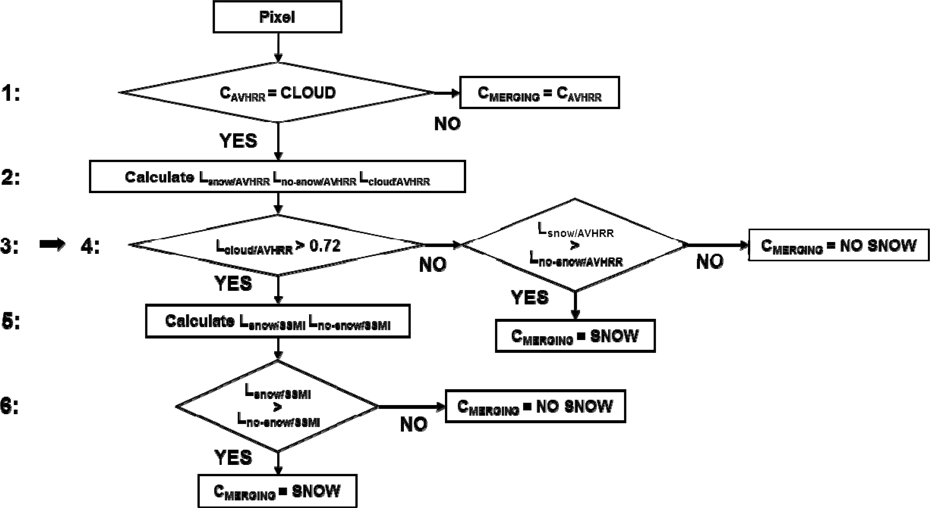
2.3. Procedure for Merging Daily AVHRR and SSM/I Snow Maps

Figure 3 illustrates the workflow of the merging procedure. Since the AVHRR sensor has a higher resolution than SSM/I, the merging algorithm gives priority to the AVHRR snow map. Thus, in the case of cloud-free pixels, the algorithm relies on the AVHRR results, even if the AVHRR and SSM/I data disagree (step 1). If a pixel is classified as a cloud in the AVHRR data, it is still possible to retrieve information on the pixel status (snow covered or snow free) from snow maps of previous and following days. For each current date, we calculate a likelihood of membership in a given class over a time window of ±4 days (see Equation (2)) (step 2). The pixel is assigned to the snow or no-snow class (whichever has the highest likelihood) if the likelihood of clouds is less than or equal to 0.72 (steps 3 and 4). If the likelihood of clouds is greater than 0.72, i.e., when the two days on either side of the central date are under cloud cover, the time window is dominated by clouds, and the results produced by the AVHRR algorithm do not enable us to draw conclusions on the presence or absence of snow. In this case, we rely on the SSM/I snow map. The likelihood of occurrence of each of the two classes (no-snow and snow) produced by the SSM/I algorithm is calculated within a time window of ±4 days from the actual day (steps 5 and 6). This is to ensure the temporal coherence of the presence/absence of snow.
The likelihood of the occurrence of a given class is defined as the sum of individual occurrences for each day of the time window. For a given class and for a given day, the individual occurrence can take the value of 1 or 0, depending on whether the pixel has been classified in this class or not. Individual occurrences are weighted according to their proximity to the central day of the window using an “inverse-distance” function, where distance is measured in days to the central day of the window. To bring the calculated likelihood values to 1, the weights are normalized to their total sum. Thus, the day before and after the date of the central time window receive the highest values, and the two days on the ends of the window receive the lowest values. For the map from the AVHRR algorithm, the calculation is as follows:
L C = i = 1 4 [ O C i × 1 | i | ] + i = 1 + 4 [ O C i × 1 i ] 2 × i = 1 4 1 i
where LC is the likelihood of class C within the time window of ±4 days of the current date, i indicates the number of days in the window and OiC indicates the occurrence of individual class C for day i (OiC = 1 if the pixel is assigned to class C; otherwise, OiC = 0).
For the snow mapping algorithm based on SSM/I data, the calculation of the likelihood is slightly different, since the date of the central window is also taken into account:
L C = i = 4 + 4 [ O C i × 1 | i | + 1 ] i = 4 4 1 | i | + 1

3. Results and Discussion

3.1. Accuracy Assessment of Snow Maps from the AVHRR Algorithm

The new time-dependent version of the AVHRR algorithm was applied to the pixel sample reserved for independent validation. Table 2 presents a comparison between these pixels as validated and as classified by the algorithm. Note that the algorithm successfully identified the three types of surface with a high success rate of around 97%. Clouds are identified with an almost perfect success rate. However, although the snow was correctly classified with a rate exceeding 93%, it was the class most affected by omission error (nearly 7% of the pixels were classified into one of the two other classes). This is explained by the fact that the algorithm is defined as a conservative algorithm regarding snow. In other words, the algorithm is based on percentiles of the snow class: snow pixels at the ends of the distribution histograms of different classification parameters are excluded in favor of the other two classes, which results in a slight underestimation of the presence of snow.
In order to verify the validity of the new version of the AVHRR algorithm, snow presence/absence derived from snow depth observations recorded at 20 meteorological stations (Figure 1) was compared to the classification results for AVHRR images for the period from 1988 to 1999 using this new algorithm. This represents a validation set of 14,640 observations (20 stations × 61 days per year × 12 years), from which 2,184 missing observations were discarded. Classification results within a 3 × 3 pixel window centered above each station were extracted, and the occurrence of each surface category inside the window was recorded. The whole window was labeled with the most frequent class in the window. Windows with a cloud cover frequency exceeding 50% were declared cloudy and excluded from the analysis (no validation information on cloudiness was available from the meteorological stations). The snow occurrence statistics were subsequently compared with snow depth observations. Results are shown in Table 3. For nearly 70% of the dates, the algorithm detected the presence of clouds. The absence of ground observations on nebulosity (cloud cover) prevents us from validating these dates. For the remaining dates, the classification algorithm correctly identified the surface status (snow, no-snow) near all stations in 90% of cases (overall success rate). This corresponds to a high-quality classification (Kappa = 0.79). The classification results for the no-snow class agreed reasonably well with ground observations, with a success rate for this class of around 92%. However, the performance of the algorithm for identifying the snow class was slightly lower than for the no-snow class, with a success rate of 87%. This is because the algorithm, as mentioned above, is more conservative for snow detection. However, these results compare favorably with similar studies. Fernandes and Zhao [29] produced daily maps of snow cover across Canada using AVHRR imagery for the period 1982 to 2005; during the spring melt period, they obtained an agreement rate higher than 87% for 50% of the validation stations. For the validation of snow depth, the authors used observations from 82 weather stations across Canada. Furthermore, Simic et al. [1] evaluated MODIS snow cover maps provided at 500-m spatial resolution with daily surface snow depth observations collected from almost 2,000 meteorological stations across Canada. They found that MODIS products showed reasonable agreement with ground data, ranging from 80% to 100%. However, the lowest agreement was obtained during snowmelt, mainly in forested areas.
The performance of the new version of the algorithm was compared to that of the former version. To do so, we used for both algorithms a snow depth dataset composed of 884 observations. This dataset was extracted from the 15 meteorological stations used for validation purposes for the initial version of the algorithm (Figure 1). It should be recalled that this version was applied to a series of images from 1987, 1992 and 1999 that covered a smaller region. The comparison results are presented in Table 4. The two versions of the algorithm show similar overall performance, with a success rate in both cases of 89%. However, the older version of the algorithm was more accurate in detecting the presence of snow than its absence (94% for snow vs. 83% for the no-snow class), whereas the new version detected the absence of snow more accurately (82% for snow against 96% for the no-snow class). For the purposes of monitoring the snow melting period, this would be to the advantage of the new version, as detection of no-snow with greater accuracy would lead to a better estimate of the end of the winter season. Another difference was that the new version detected the presence of clouds for 20% more dates than the old one did. Because of the already noted lack of ground-based information on cloudiness, it is impossible to evaluate the two versions in this respect. However, the new version showed a high accuracy for detecting clouds in the pixel-based validation test (Table 2).

3.2. Accuracy Assessment of Snow Maps from the SSM/I Algorithm

The mapping results for the SSM/I algorithm were also validated using the 20 meteorological stations (Figure 1). The dataset used covered the entire study period (1988–1999), but comprised only 9,476 valid observations. This was due to incomplete data at some of the stations and the fact that data from some sites were not usable, due to contamination of the corresponding SSM/I pixel by surface water (at coastal stations or near large water bodies). Validation results are presented in Table 5. It turns out that the SSM/I algorithm detected the presence of snow with a higher success rate than the AVHRR algorithm (95% vs. 87%). However, on the whole, it performed less well than the AVHRR algorithm, with an overall success rate of 83% compared to 90% for the AVHRR algorithm. It correctly detected snow-free surfaces in only 75% of cases. In addition, 28% of the surfaces identified as snow-covered were, in fact, snow-free. This commission error resulted in an overestimation of snow surfaces and, therefore, an overestimation of the date of the end of the winter season. It should also be noted that validation of this approach remains problematic, because of the differences in the nature of the data used (point observations vs. 25 × 25 km pixels). With a 25-km SSM/I pixel only partly covered by snow, so with a mixed signature, this can be interpreted as snow by the algorithm, while no snow was present anymore at the weather station, giving a surface identified as snow covered while it is it in fact snow free. The opposite case could also happen if snow is still present at the weather station, but not elsewhere.

3.3. Accuracy Assessment of the Merging Algorithm

Figure 4 shows an example of snow mapping results using four different algorithms: the two individual mapping algorithms (AVHRR and SSM/I) and two different merging strategies (simple and temporal merging). The simple merging strategy uses the SSM/I results whenever the AVHRR algorithm detects clouds. The second strategy is the proposed methodology (described above). In the example shown, the simple merging strategy seems to successfully capture the spatial distribution of snow cover. Thus, the frontier line of snow is well defined, especially in cases where the information comes from AVHRR data (better spatial resolution). The SSM/I data replace the information missing from the vast stretch of territory covered by clouds in the center of the AVHRR image. However, since the SSM/I algorithm does not work over water pixels, data for the pixels corresponding to the coastline and large water bodies remain missing. In contrast, the proposed merging approach fills the data gaps corresponding to these pixels over much of the territory, in particular, on the Labrador coast and the Gaspé Peninsula. Better yet, the temporal merging of the algorithm does a better job of defining the snow frontier line. This frontier is located further north than suggested by the SSM/I algorithm, apparently because the SSM/I algorithm mistook rather patchy snow covered areas for continuous snow cover, due to its tendency to overestimate the presence of snow compared to the AVHRR algorithm.
The snow mapping results produced using the merging algorithm were compared with ground observations over the time period 1988–1999, as described above. The results are presented in Table 6. The algorithm correctly identified the surface conditions (snow, no-snow) at stations in 86% of the cases, which represents a very satisfactory score (Kappa = 0.72). However, its overall performance level was intermediate between that of the AVHRR and SSM/I algorithms. With respect to its performance in detecting both types of surfaces individually, the merging algorithm seems to mitigate the weaknesses of each algorithm without, however, fully benefitting from their strengths. Accordingly, the success rate of snow detection increased from 87%, in the case of AVHRR, to 90%, but did not reach the SSM/I success rate of 95%. In addition, the success rate of no-snow detection rose from 75%, in the case of SSM/I, to 84%, but did not reach the 92% success rate of the AVHRR algorithm. The merging algorithm also showed better performance than the SSM/I algorithm with respect to the commission error on snow, as it dropped from 28%, in the case of the latter algorithm, to 19% for the merging algorithm.
However, this performance is still very satisfactory compared with similar work. Simic et al. [1] validated, across Canada, the NOAA snow mapping product combining data from the GOES optical sensor and the SMM/I passive microwave sensor (with a nominal spatial resolution of 4 km). They found that the product shows the lowest success rate during the melting season (80%). They also reported an overestimation of the presence of snow, due to wet snow during this period that affects the quality of snow detection using microwave data. Liang et al. [17] and Gao et al. [18] combined MODIS and AMSRE data and tested their algorithms over Xinjiang (China) and Alaska (USA), respectively; they obtained 75% and 86% overall accuracy for this blended product, respectively.
The date of the end of the melting season (corresponding to the total disappearance of snow cover) was determined from daily snow maps derived using the merging algorithm, for each of the 20 stations used for validation and each year of the study period (1988–1999). This allowed the difference to be calculated between the date of the end of the season, as estimated from satellite imagery, and that obtained from snow depth observations. Statistics on the differences between the two dates are presented in Table 7. It appears from the results that the merging algorithm allows the end of the season to be estimated globally without bias from the actual date (snow depth observation). This is also true for each year of the study period, since all individual mean day difference values are less than one standard deviation away from zero. This implies that the calculated mean values are not statistically different from zero. It also indicates that the proposed merging algorithm could be used to monitor snow extent over time and to estimate the end of the melting season with fairly good confidence, which is of great importance in northern hydrology and climatology.
Ground observations at meteorological stations and/or snow courses remain the most reliable and commonly used source of information on the actual presence of snow. However, validation of such an algorithm using ground observations implies comparing point information with information integrated over several square kilometers (1 × 1 km, in the case of AVHRR, and 25 × 25 km for SSM/I), which is not optimal. It would therefore be interesting to use surface-based information (rather than point-based information) on snow extent, which can be used as a reference dataset for validation purposes. Thus, in addition to the ground-based observations, snow maps produced using the proposed merging approach were also validated spatially using Landsat-TM imagery (data distributed by the Land Processes Distributed Active Archive Center (LP DAAC), located at USGS/EROS, Sioux Falls, SD, USA. http://lpdaac.usgs.gov). The Landsat images were selected so as to be distributed as evenly as possible over the study area and to cover the main land cover types (Figure 5). They were processed beforehand to produce high-resolution snow maps using a newly developed snow detection approach [30]. This is a modified version of the SNOWMAP algorithm [7,8,3133], which is based on the joint use of the NDSI (Normalized Difference Snow Index) and the NDVI (Normalized Difference Vegetation Index).
In the initial version of SNOWMAP, a minimum threshold value of 0.1 is used for NDVI, regardless of the value of NDSI, to eliminate water and ice. Unfortunately, this leads to the elimination of all the snow-covered areas with low vegetation (e.g., high altitude areas without vegetation or covered with a snow layer that exceeds the herbaceous vegetation). Moreover, this version ignores a very important component of the cryosphere: ice on inland water. This cryospheric component is very dynamic in time and space, and it plays a very important role in climate feedback mechanisms; therefore, it cannot be neglected, especially in a territory, such as Eastern Canada, which is characterized by a myriad of lakes, ponds and rivers. Therefore, Chokmani et al. [30] proposed a modified version of SNOWMAP, which does not include the minimum NDVI value of 0.1. Moreover, the lower limit of the acceptance zone, introduced by Klein et al. [32], was extrapolated to NDVI values of less than 0.1. Thus, the modified SNOWMAP allows snow-covered areas with low NDVI values, as well as ice on inland water bodies to be correctly identified. Despite the introduction of this new zone of acceptance, detection of snow in coniferous forests remains unsatisfactory. Chokmani et al. [30] introduced a spatial correction procedure to extend snow detection results from open areas to adjacent coniferous forests and mixed stand areas, based on the fact that the snow cover melts later in forests than in open areas.
Figure 6 shows snow maps of the regions depicted in the six Landsat validation images produced using the studied algorithms. The percentage of snow cover calculated by the snow mapping algorithm using Landsat-TM imagery was compiled and compared with maps produced using the proposed merging algorithm (Table 8). Examination of the results reveals the following findings:
(1).
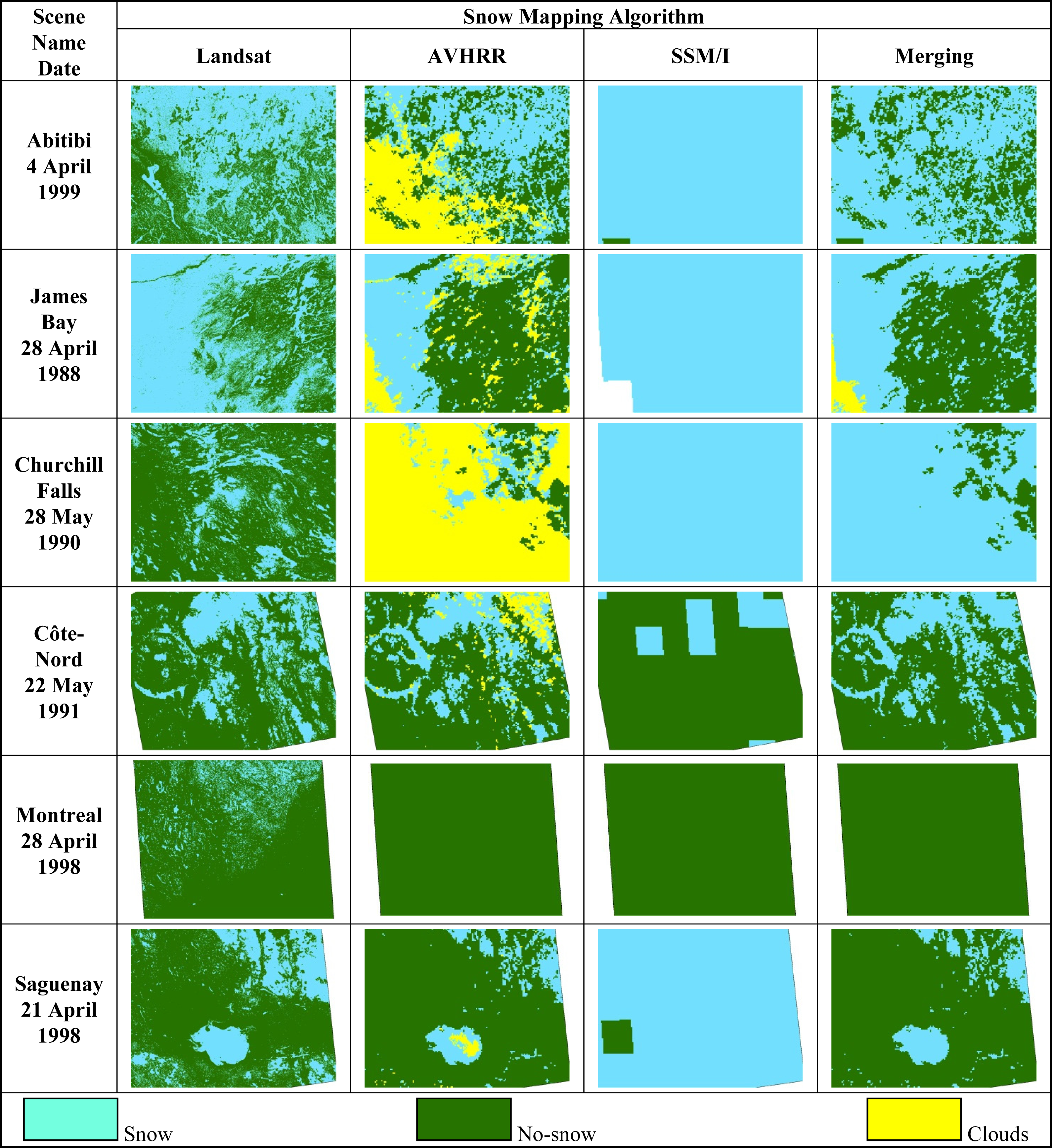
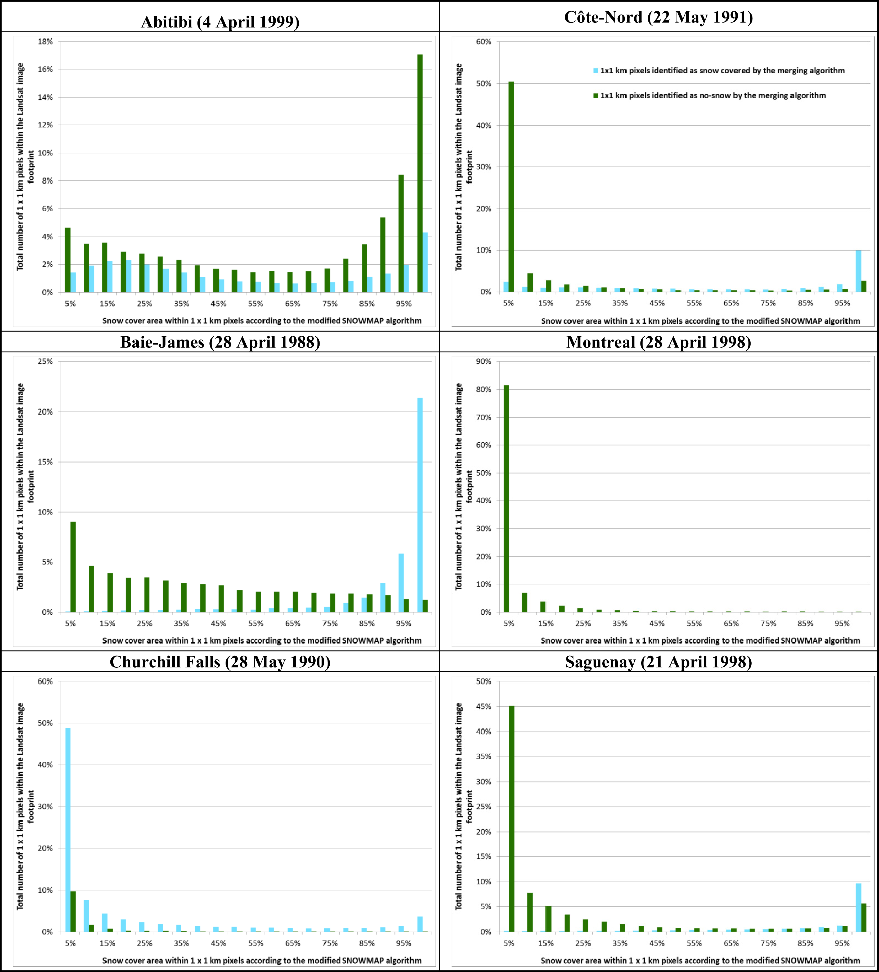
When the AVHRR scenes are dominated by clouds (Figure 6: Abitibi and Churchill Falls), the merging algorithm tends to overestimate the presence of snow. This corroborates the 19% commission error reported in Table 6. The greater the cloud cover, the greater the error. For the Abitibi and Churchill Falls scenes, snow cover was overestimated by about 12% and 48%, respectively (Table 8). For these two scenes, the snow maps produced by the merging algorithm for cloud-free areas, which, in fact, comes from the AVHRR algorithm, were similar to the high-resolution maps from Landsat imagery (considered as reference data). By contrast, cloud-covered areas were mostly filled by the map derived from the SSM/I algorithm, which, unlike the reference maps, detected snow for both of the two scenes.
(2).
Under the cloud-free conditions, where the maps produced by the merging algorithm were derived from the AVHRR algorithm, snow cover extent was underestimated over certain scenes: James Bay (−22%), Saguenay (−13%) and Montreal (−4%) (Table 8). These were areas of discontinuous snow cover (see corresponding reference map: the central part of the James Bay scene, the northern part of the Montreal scene and the southern part of the Saguenay scene). This partly explains the merging algorithm’s omission error for snow detection (Table 6). In the absence of discontinuous snow cover, as in the Côte-Nord scene (Figure 6), the results of the merging algorithm are consistent with snow cover maps from Landsat imagery. The difference between the two snow cover extents was about 2% (Table 8).
To analyze the sensitivity of the merging algorithm to detect the presence of snow at the sub-pixel level, snow cover fraction (SCF) was calculated for each 1 × 1 km pixel within each Landsat scene footprint by compiling statistics for snow detection using the modified SNOWMAP algorithm from the high resolution imagery (30 × 30 m). Therefore, the statistics for snow detection by the merging algorithm were plotted according to the SCF classes thus obtained, with a 5% increment (Figure 7).
Firstly, it should be noted that for the scenes with clouds (Churchill and Abitibi Falls), the merging algorithm predominantly produced snow pixels regardless of the SCF calculated with high resolution imagery. This is most obvious with the Churchill Falls scene showing the heaviest cloud cover. Regarding the Abitibi scene, this overestimation seems to only affect the SCF values less than 25–30%. This corresponds to the southwestern part of the scene obstructed by clouds, which happens to be an area of low SCF values, with the exception of Lake Abitibi, which was still covered with ice at that date (see corresponding thumbnail images in Figure 6). By examining “cloud-free” scenes, it turns out that the merging algorithm starts detecting snow predominantly from SCF values higher than 30–35% for scenes dominated by dense coniferous forest (Côte-Nord in Figure 7), while for scenes dominated by more open land (Saguenay and Abitibi in Figure 7), this threshold is about 80–85% of SCF (Figure 7). At first glance, this seems inconsistent with the physics of the phenomenon, since snow detection should normally be easier in open areas (corresponding to lower detection threshold SCF values) compared with closed forest environments, such as dense needleleaf forest, and not the opposite. This could be explained by the fact that the high-resolution snow maps have the same limitation in snow detection in closed environments. Indeed, even if the algorithm used, the modified SNOWMAP, comprises a spatial correction to improve the detection of snow under forest cover, this correction is insufficient and needs to be improved [30]. Thus, the SCF calculated for these areas would be underestimated. Therefore, we should rely on the statistics obtained from the scenes in an open environment. Accordingly, the sensitivity of the merging algorithm, rather, would be 80% of SCF. As such, 100% of the pixels in the Montreal scene have less than 35% of SCF. Therefore, the whole scene was classified as snow free by the fusion algorithm. These findings are consistent with the point-based validation results and would explain the origin of the omission error for snow detection by the merging algorithm (Table 6).

4. Conclusions

In this paper, the development and validation of algorithms for historical mapping of daily snow cover, over the period 1988–1999, in Eastern Canada from NOAA-AVHRR and SSM/I images were discussed. This includes: (1) an algorithm for snow detection using NOAA-AVHRR images and integrating temporal variation in detection thresholds; (2) a new version of the algorithm for snow detection using passive microwave data (SSM/I), modified to make it sensitive to the presence of wet snow; and (3) a merging algorithm that combines snow maps produced by the first two algorithms. The results of these different algorithms were validated using snow depth observations and high spatial resolution snow maps from Landsat-TM imagery. The snow mapping algorithm was focused on the most critical period, i.e., the spring melt season, between April 1st and May 31st of each year.
According to the snow depth observations, the AVHRR algorithm correctly identified surface conditions (snow, no-snow) with a high overall success rate (90%). However, detection of snow, although also highly successful (exceeding 87%), was more affected by omission errors than the detection of snow-free areas (13% vs. 8%, respectively). This is expected, since the algorithm is, by definition, conservative with respect to the snow. It is therefore proposed that the values of the different thresholds be established at an intermediate level between the snow class and competing class (no-snow or clouds) instead of being calculated only from percentiles of the calibration snow sample.
By contrast, the SSM/I algorithm performed slightly less well, with an overall success rate of 83%, despite its better performance in snow detection (success rate of 95%). Moreover, this high success rate was marred by a high commission error (28%), resulting in a strong tendency to overestimate snow cover extent. It seems that the change made to the original version of the algorithm to improve its sensitivity to wet snow (the introduction of the gradient of the emissivity instead of the temperature gradient), results in an overestimation of the snow extent. Therefore, the detection threshold based on the emissivity gradient should be reviewed in order to correct this bias.
The combination of the snow mapping results from the AVHRR and SSM/I algorithms using temporal merging produced maps that benefit from both the high-resolution capabilities of AVHRR and the insensitivity of SSM/I to the presence of clouds. This enabled us to correctly detect snow and no-snow surfaces with a high overall success rate of 86% (90% for snow and 84% for no-snow). Moreover, the merging algorithm allows the end date of the melt season to be calculated without almost any bias compared to observed end dates at meteorological stations, with a standard deviation of about 11 days. In comparison to high-spatial-resolution snow maps produced from Landsat-TM imagery (30-m resolution), the merging algorithm showed an overestimation of the snow extent in the presence of persistent cloud cover (more than three consecutive days), when the detection relies only on SSM/I data. Under clear sky conditions, the algorithm relies on AVHRR data and tends to underestimate snow extent when the snow cover within the field of view of the AVHRR sensor is patchy. Based on high-spatial-resolution snow maps over open environments (deciduous forest and open land), it seems that the algorithm starts detecting snow predominantly within the AVHRR pixels when the snow cover occupies more than 80% of the field of view.

Acknowledgments

This research was funded by the Natural Sciences and Engineering Research Council of Canada (NSERC), the OURANOS Consortium on regional climatology and adaptation to climate change and Hydro-Quebec. The authors would like to gratefully acknowledge them for their financial support. The authors also thank L.M. Pâquet, P. Boccage and N.Y. Sena for their assistance. In addition, the authors thank the anonymous reviewers for their valuable comments.

Conflict of Interest

The authors declare no conflict of interest.

References and Notes

  1. Simic, A.; Fernandes, R.; Brown, R.; Romanov, P.; Park, W. Validation of VEGETATION, MODIS, and GOES+SSM/I snow cover products over Canada based on surface snow depth observations. Hydrol. Process 2004, 18, 1089–1104. [Google Scholar]
  2. Frei, A. A new generation of satellite snow observations for large scale earth system studies. Geogr. Compass 2009, 3, 879–902. [Google Scholar]
  3. Chen, C.; Lakhankar, T.; Romanov, P.; Helfrich, S.; Powell, A.; Khanbilvardi, R. Validation of NOAA-interactive multisensor snow and Ice Mapping System (IMS) by comparison with ground-based measurements over continental United States. Remote Sens 2012, 4, 1134–1145. [Google Scholar]
  4. Ramsay, B.H. The interactive multisensor snow and ice mapping system. Hydrol. Process 1998, 12, 1537–1546. [Google Scholar]
  5. Romanov, P.; Gutman, G.; Csisar, I. Automated monitoring of snow cover over North America with multispectral satellite data. J. Appl. Meteorol 2000, 39, 1866–1880. [Google Scholar]
  6. Bitner, D.; Carroll, T.; Cline, D.; Romanov, P. An assessment of the differences between three satellite snow cover mapping techniques. Hydrol. Process 2002, 16, 3723–3733. [Google Scholar]
  7. Hall, D.K.; Rhoads, J.D.; Salomonson, V.V. Development of methods for mapping global snow cover using Moderate Resolution Imaging Spectroradiometer data. Remote Sens. Environ 1995, 54, 127–140. [Google Scholar]
  8. Hall, D.K.; Riggs, G.A.; Salomonson, V.V.; DiGirolamo, N.E.; Bayr, K.J. MODIS snow-cover products. Remote Sens. Environ 2002, 83, 181–194. [Google Scholar]
  9. Dietz, A.J.; Kuenzer, C.; Gessner, U.; Dech, S. Remote sensing of snow—A review of available methods. Int. J. Remote Sens 2012, 33, 4094–4134. [Google Scholar]
  10. Notarnicola, C.; Duguay, M.; Moelg, N.; Schellenberger, T.; Tetzlaff, A.; Monsorno, R.; Costa, A.; Steurer, C.; Zebisch, M. Snow cover maps from MODIS images at 250 m resolution, part 1: Algorithm description. Remote Sens 2013, 5, 110–126. [Google Scholar]
  11. Solberg, R.; Wangensteen, B.; Amlien, J.; Koren, H.; Metsämäki, S.; Nagler, T.; Luojus, K.; Pulliainen, J. A New Global Snow Extent Product Based on ATSR-2 and AATSR. Proceedings of 2010 IEEE International Geoscience and Remote Sensing Symposium (IGARSS), Honolulu, HI, USA, 25–30 July 2010; pp. 1780–1783.
  12. Chokmani, K.; Bernier, M.; Gauthier, Y. Suivi spatio-temporel du couvert nival du Québec à l’aide des données NOAA-AVHRR. Revue des Sciences de l'Eau 2006, 19, 163–179. [Google Scholar]
  13. Chokmani, K.; Bernier, M.; Slivitzky, M. Validation of a method for snow cover extent monitoring over Quebec (Canada) using NOAA-AVHRR data. EARSeL eProc 2005, 4, 106–118. [Google Scholar]
  14. Langlois, A. Étude de la Variation Spatio-Temporelle du Couvert Nival par Télédétection Micro-Ondes Passives et Validation du Modèle Régional Canadien du Climat (MRCC). Université de Sherbrooke, Sherbrooke, QC, Canada, 2003. [Google Scholar]
  15. Langlois, A.; Royer, A.; Fillol, E.; Frigon, A.; Laprise, R. Evaluation of the snow cover variation in the Canadian regional climate model over eastern Canada using passive microwave satellite data. Hydrol. Process 2004, 18, 1127–1138. [Google Scholar]
  16. Caya, D.; Laprise, R. A semi-implicit semi-lagrangian regional climate model: The Canadian RCM. Mon. Wea. Rev 1999, 127, 341–362. [Google Scholar]
  17. Liang, T.; Zhang, X.; Xie, H.; Wu, C.; Feng, Q.; Huang, X.; Chen, Q. Toward improved daily snow cover mapping with advanced combination of MODIS and AMSR-E measurements. Remote Sens. Environ 2008, 112, 3750–3761. [Google Scholar]
  18. Gao, Y.; Xie, H.; Lu, N.; Yao, T.; Liang, T. Toward advanced daily cloud-free snow cover and snow water equivalent products from Terra-Aqua MODIS and Aqua AMSR-E measurements. J. Hydrol 2010, 385, 23–35. [Google Scholar]
  19. Cordisco, E.; Prigent, C.; Aires, F. Sensitivity of Satellite Observations to Snow Characteristics. Proceedings of 2003 IEEE International Geoscience and Remote Sensing Symposium (IGARSS), Toulouse, France, 21–25 July 2003.
  20. Koskinen, J.; Metsamaki, S.; Grandell, J.; Janne, S.; Matikainen, L.; Hallikainen, M. Snow monitoring using radar and optical satellite data. Remote Sens. Environ 1999, 69, 16–29. [Google Scholar]
  21. Tait, A.; Barton, J.S.; Hall, D.K. A prototype MODIS-SSM/I snow-mapping algorithm. Int. J. Remote Sens 2001, 22, 3275–3284. [Google Scholar]
  22. Brodzik, M.J.; Armstrong, R.L.; Savoie, M. Global EASE-Grid 8-Day Blended SSM/I and MODIS Snow Cover; National Snow and Ice Data Center: Boulder, CO, USA, 2007. [Google Scholar]
  23. Latifovic, R.; Trishchenko, A.P.; Chen, J.; Park, W.B.; Khlopenkov, K.V.; Fernandes, R.; Pouliot, D.; Ungureanu, C.; Luo, Y.; Wang, S.; et al. Generating historical AVHRR 1 km baseline satellite data records over Canada suitable for climate change studies. Can. J. Remote Sens 2005, 31, 324–346. [Google Scholar]
  24. Voigt, S.; Koch, M.; Baumgartner, M.F. A multichannel threshold technique for NOAA AVHRR data to monitor the extent of snow cover in the Swiss Alps. IAHS-AISH Publ 1999, 256, 35–43. [Google Scholar]
  25. Chokmani, K.; Bernier, M.; Beaulieu, V.; Philippin, M.; Slivitzky, M. Suivi Spatio-Temporel du Couvert Nival à l’Aide des Données NOAA-AVHRR; R-719; Institut National de la Recherche Scientifique-Eau, Terre et Environnement: Québec, QC, Canada, 2004; p. 73. [Google Scholar]
  26. Mialon, A.; Fily, M.; Roy, A. Seasonal snow cover extent from microwave remote sensing data: Comparison with existing ground and satellite based measurements. EARSeL eProc 2005, 4, 215–225. [Google Scholar]
  27. Côté, J.; Gravel, S.; Méthot, A.; Patoine, A.; Roch, M.; Staniforth, A. The operational CMC-MRB global environmental multiscale (GEM) model. Part I: Design considerations and formulation. Mon. Wea. Rev 1998, 126, 1373–1395. [Google Scholar]
  28. Royer, A.; Goïta, K.; Kohn, J.; De Sève, D. Monitoring dry, wet, and no-snow conditions from microwave satellite observations. IEEE Geosci. Remote Sens. Lett 2010, 7, 670–674. [Google Scholar]
  29. Fernandes, R.; Zhao, H. Mapping Daily Snow Cover Extent over Land Surfaces Using NOAA AVHRR Imagery. Proceedings of 5th EARSeL Workshop: Remote Sensing of Land Ice and Snow, Bern, Switzerland, 11–13 February 2008; pp. 1–8.
  30. Chokmani, K.; Dever, K.; Bernier, M.; Gauthier, Y.; Paquet, L.M. Adaptation of the SNOWMAP algorithm for snow mapping over eastern Canada using Landsat-TM imagery. Hydrol. Sci. J 2010, 55, 649–660. [Google Scholar]
  31. Hall, D.K.; Riggs, G.A.; Salomonson, V.V. Algorithm Theoretical Basis Document (ATBD) for the MODIS Snow and Sea Ice-Mapping Algorithms. Available online: http://eospso.nasa.gov/sites/default/files/atbd/atbd_mod10.pdf (accessed on 23/10/2013).
  32. Klein, A.G.; Hall, D.K.; Riggs, G.A. Improving snow cover mapping in forests through the use of a canopy reflectance model. Hydrol. Process 1998, 12, 1723–1744. [Google Scholar]
  33. Riggs, G.; Hall, D.K. Snow Mapping with the MODIS Aqua Instrument. Proceedings of 61st Eastern Snow Conference, Portland, ME, USA, 9–11 June 2004; pp. 81–84.
Figure 1. Location of the study area and the meteorological stations used in snow map validation.
Remotesensing 05 05463f1
Figure 2. Flow chart of the AVHRR algorithm (reprinted from [13]). NDVI, Normalized Difference Vegetation Index.
Remotesensing 05 05463f2
Figure 3. Flowchart of the decision process for merging AVHRR and SSM/I snow maps: CALGORITHM represents the pixel’s class according to the algorithm and L, the class’s likelihood according to a given algorithm within a ±4 day window (Equation (2)).
Remotesensing 05 05463f3
Figure 4. Snow maps for 19 April 1991 using AVHRR, SSM/I, a simple merging algorithm and the proposed merging algorithm.
Remotesensing 05 05463f4
Figure 5. Location of the selected Landsat-TM images.
Remotesensing 05 05463f5
Figure 6. Snow maps for the Landsat validation scenes produced using the algorithms . The presence of clouds in some AVHRR scenes and not in the corresponding Landsat scenes, despite the fact that both scenes were acquired on the same date, is explained by the fact that the snow mapping algorithm used with Landsat images is a “cloud-free” algorithm. The spatial correction procedure included in the new version of SNOWMAP allows the areas obstructed by clouds to be mapped [30]. In addition, the two images are acquired at different time. Landsat images are acquired at around 10:00 a.m. local time, while the AVHRR images are acquired early in the afternoon, between 1:00 p.m. and 3:00 p.m. local time.
Remotesensing 05 05463f6
Figure 7. Snow detection by the merging algorithm, compared to the snow cover fraction produced by the modified SNOWMAP algorithm, integrated over a 1 × 1 km cell size.
Remotesensing 05 05463f7
Table 1. Threshold values of the AVHRR algorithm. DOY, day of year.
ThresholdThreshold as a Function of DOY
(1)
T4max
99th percentile of T4 from snow calibration pixels
Remotesensing 05 05463i1
T4max = 1.68 × 10⁻³ × DOY2 − 0.21 × DOY + 281.5
(2)
T4min
1st percentile of T4 from snow calibration pixels
Remotesensing 05 05463i2
T4min = 0.36 × 10⁻³ × DOY2 + 0.09 × DOY + 247.4
(3)
ΔT45max
Time independent
ΔT45max = 2 °K
(4)
NDVImax
99th percentile of NDVI from snow calibration pixels
Remotesensing 05 05463i3
NDVImax = 0.13 × 10⁻³ × DOY2 − 0.03 × DOY + 1.83
(5)
ΔT34max
95th percentile of T3–T4 from snow calibration pixels
Remotesensing 05 05463i4
ΔT34max = 2.70 × 10⁻³ × DOY2 − 0.61 ×DOY + 40.97
(6)
A1min
1st percentile of A1 from snow calibration pixels
Remotesensing 05 05463i5
A1min = −0.05 × 10⁻³ × DOY2 + 0.01 × DOY −0.36
Table 2. Pixel-based validation of the new AVHRR algorithm using the independent validation sample.
Total Pixels Used in ValidationClassification
SnowNo-SnowClouds

ValidationSnow62,43093%4%3%
No-snow14,5331%98%1%
Clouds62,5420%0%100%
Overall success rate97%
Table 3. Validation of the new version of the AVHRR algorithm using ground observations of snow from the 20 validation meteorological stations for the period 1988–1999.
Classification
SnowNo-SnowCloudsTotal
ObservationsSnow1,3792151,594

No-snow1742,0612,235

Total1,5532,2768,62712,456


Success rateOmission ErrorCommission Error

Snow87%13%11%
No-snow92%8%9%


Overall success rate90%
Kappa coefficient0.79
Table 4. Validation of the two versions of the AVHRR algorithm using the same ground snow observations from 15 meteorological stations for 1987, 1992 and 1999.
a) Initial VersionClassification
SnowNo-SnowCloudsTotal

ObservationsSnow22213235
No-snow35168203
Total257181446884


Success RateOmission ErrorCommission Error

Snow94%6%14%
No-snow83%17%7%

Overall success rate89%
Kappa coefficient0.78


b) New versionClassification
SnowNo-SnowCloudsTotal

ObservationsSnow13630166
No-snow7177184
Total143207534884


Success RateOmission ErrorCommission Error
Snow82%18%5%
No-snow96%4%14%


Overall success rate89%
Kappa coefficient0.79
For comparison purposes, we only used the 15 stations that were used to validate the original version of the algorithm.
Table 5. Validation of the SSM/I algorithm using ground observations of snow from the 20 validation meteorological stations for the period from 1988 to 1999.
Classification
SnowNo-SnowTotal
ObservationsSnow3,5831943,777
No-snow1,4134,2865,699
Total4,9964,4809,476


Success RateOmission ErrorCommission Error

Snow95%5%28%
No-snow75%25%4%


Overall success rate83%
Kappa coefficient0.66
Table 6. Validation of the merging algorithm using snow ground observations from the 20 validation meteorological stations for the period 1988–1999.
Classification
SnowNo-SnowTotal
ObservationsSnow4,7215295,250
No-snow1,1355,7466,881
Total5,8566,27512,131


Success RateOmission ErrorCommission Error
Snow90%10%19%
No-snow84%16%8%


Overall success rate86%
Kappa coefficient0.72
Table 7. Statistics on the difference between the date of the end of the melt season (DEMS), as estimated from satellite imagery using the merging algorithm, and that calculated from snow depth observations at the 20 meteorological stations.
Year[Estimated DEMS] − [Observed DEMS] (in days)
Mean ValueStandard Deviation
19885.513.9
19891.610.6
19900.98.2
19915.87.8
19922.112.2
1993−6.79.8
19941.98.1
1995−0.27.1
1996−3.312.0
1997−2.411.0
1998−3.610.1
1999−0.28.5

All years−0.110.7
Table 8. Percentage of snow cover in the six Landsat-TM footprints, calculated from snow maps generated from the Landsat-TM imagery and maps produced by the proposed merging algorithm (from April 1 to May 31 of each year).
Scene Name Date Remotesensing 05 05463i6 Landsat Remotesensing 05 05463i7 MergingPercentage of Landsat Footprint Covered by Snow
Abitibi
4 April 1999
Remotesensing 05 05463i8Landsat60%
Merging72%
Merging − Landsat12%
Baie-James
28 April 1988
Remotesensing 05 05463i9Landsat58%
Merging36%
Merging − Landsat−22%
Churchill Falls
28 May 1990
Remotesensing 05 05463i10Landsat17%
Merging65%
Merging − Landsat48%
Côte-Nord
22 May 1991
Remotesensing 05 05463i11Landsat27%
Merging29%
Merging − Landsat2%
Montreal
28 April 1998
Remotesensing 05 05463i12Landsat04%
Merging00%
Merging − Landsat−04%
Saguenay
21 April 1998
Remotesensing 05 05463i13Landsat31%
Merging18%
Merging − Landsat−13%

