Time-Space Variability of Chlorophyll-a and Associated Physical Variables within the Region off Central-Southern Chile

Abstract

Time-space fluctuations of chlorophyll-a (Chl-a) within the region off central-southern Chile (33–42°S), and their association with meteorological-oceanographic conditions, were analyzed using satellite time series data (2002–2012). The mean distribution of moderate values of Chl-a (∼0.5 mg·m⁻³) in the northern section (33–38°S) extended out to ∼200 km of the coast whereas they were restricted to a narrower band in the southern section (38–42°S). Mean wind stress and wind stress curl were upwelling favorable for most part of the year in the northern section whereas upwelling-downwelling periods were distinct in the southern section. The dominant frequency of Chl-a variability in the coastal zone and the coastal transition zone was annual, as it was for the rest of the variables, except in a transitional band between these zones and where a semi-permanent jet is located. At the annual frequency, the alongshore distribution of coastal Chl-a presented strong discontinuities, with minimum values around upwelling centers (∼37 and 40°S) and higher values (> 2 mg·m⁻³) in between. Also at the annual frequency, correlation analyses suggest that Ekman transport and Ekman pumping might act synchronously to extend the offshore distribution of the highest Chl-a values during the spring-summer period whereas mesoscale activity appears to contribute to Chl-a increases in the coastal transition zone. Sea surface temperature does not appear to be associated with the annual cycle of Chl-a in the coastal zone and in the coastal transition zone it might be linked to Chl-a variability through the effects of internal waves.

1. Introduction

Eastern Boundary Current (EBC) systems, including those off South America (Humboldt Current System, HCS; ∼5–45°S), the NW Iberian Peninsula, NW Africa (Canary Current System), SW Africa (Benguela System), and off NW America (the California Current System), all display significant temporal and spatial variation [1,2]. These highly dynamic environments have many common dominant physical processes but also have important differences within and between them. In the temporal dimension, the EBCs display differences between and/or within them with respect to the dominant modes of variability, the most significant of which are the semiannual, intraseasonal, seasonal, annual, and/or interannual scales [3,4].

Coastal upwelling occurs recurrently or semi-permanently during the year in EBCs at lower latitudes whereas it is a highly seasonal process in EBCs of mid- to high latitudes [2,4]. A seasonal development or a synoptic increase in upwelling favorable wind stress conditions has frequently been associated with a significant nutrient input to the surface layer in the coastal zone and, in turn, with an enhancement in biological production, in particular, an increase in phytoplankton biomass or bloom formation [5–7]. However, other physical processes (e.g., sea level, wind stress curl, mesoscale activity, mixed layer depth) with seasonal variability can be more relevant in producing enhancements in phytoplankton biomass in the coastal zone and/or in the adjacent CTZ [3,4,8–11].

Significant alongshore (latitudinal) and across-shore (coastal-oceanic) variability in coastal upwelling conditions between and within the main EBCs has also been described. These differences arise from latitudinal variation in large scale wind systems and/or from local variations in wind forcing linked to coastal topography, coastline orientation, and/or bathymetry; in addition, variations in large-scale circulation and mesoscale activity, and continental runoff can have a significant influence [11–15]. Geographical and/or local changes in the distribution of phytoplankton biomass and/or biological production rates have been positively related to spatial variability in wind-driven coastal upwelling [7,15,16] but, in some cases, this association has been found to be weak or negative [17,18]. The level of mesoscale activity (in terms of eddy kinetic energy) has been identified as an additional forcing factor causing cross-shore differences in the distribution of nutrients and/or phytoplankton (biomass and primary production rates) between and within EBCs [12,19,20].

In the HCS, the patterns of spatial and temporal variability of surface Chl-a have been described in previous studies using different satellite datasets and time-space resolutions, as well as different periods of analysis and/or regions of study [3,6,8,21,22]. In the most recent satellite color time series study for the HCS (11 years: 1997–2007; 10–40°S), the annual and interannual scales of variability in Chl-a were found to be dominant [10]. Wind stress and Rossby wave propagation appear to modulate the annual Chl-a signal in the coastal zone and in the adjacent coastal transition zone; interannual Chl-a variability was closely associated with El Niño perturbations [10]. Results of this study [10] also revealed that, within the HCS, Chl-a time-space distribution and variability, and the associated forcing factors, were clearly distinct in 3 regions: off Peru (10–18°S), northern Chile (18–30°S) and central-southern Chile (30–40°S).

The region off central-southern Chile between 33 and 42°S (Figure 1), one of the most productive in the HCS, is characterized by a complex bathymetry which includes shallower ocean areas (e.g., the Itata Terrace), canyons (e.g., Itata and Bio-Bio canyons), a trench (Peru-Chile Trench), embayments (e.g., Gulf of Arauco, Concepcion Bay), and islands (e.g., Mocha and Santa María Islands). Several capes (e.g., P. Lavapié, P. Falsa) and rivers (e.g., Bio-Bio, Calle-Calle) are found within this region. The width of the continental shelf varies from ∼30 km to ∼100 km and the coastline has a strong north-south orientation in the southern section (south of 37°S) and a northeast-southwest orientation in the northern section.

Coastal upwelling in the region off central-southern Chile is mostly concentrated during the austral spring-summer period (mid-September to mid-March), when alongshore winds from the south or southwest are dominant [23–25]. In the most southern section, and further south (∼45°S), winds associated with the West Wind Drift are mostly perpendicular to the coast [26]. In the offshore region, wind stress curl is mostly anticyclonic (downwelling favorable) whereas in the coastal zone is mostly cyclonic (upwelling favorable) and is intensified during the spring-summer period [27]. The alongshore circulation pattern in the region includes an equatorward coastal current with characteristics of a jet (>10 cm·s⁻¹), especially strong during the spring-summer period [22,28,29]. Mesoscale activity amplifies the annual cycle of satellite Chl-a in the region off central-southern Chile [10]. In addition, the annual cycle of satellite Chl-a displays opposite phases in the coastal zone and offshore of it, including the coastal transition and the oceanic zones), with maximum Chl-a values during the spring-summer upwelling period in the first and during the winter in the second [6,10]. In situ studies of phytoplankton variability have focused on the annual scale of variability in the coastal zone; a strong association between seasonal upwelling and the annual maximum in phytoplankton biomass, including Chl-a concentration, has been found [30–34]. Within this region, however, the time-space variability of phytoplankton communities, including Chl-a as phytoplankton biomass, and the physical factors that influence this variability, have not been characterized yet.

In this study, the time-space variability of satellite Chl-a within the region between 33 and 42°S and from the coast to 76°W was evaluated and the potential physical forcing behind such variability was explored. A decade of satellite time series data (2002–2012) was used for the following purposes: (i) to characterize the mean distribution of surface Chl-a and of physical variables potentially forcing Chl-a variability; (ii) to identify the dominant frequencies in their temporal variability; (iii) to evaluate alongshore and across-shore differences in their patterns of variability at the dominant frequencies; and (iv) to explore the association between time-space variability in Chl-a and the physical variables. The emphasis of the analyses was placed on the spatial variability of Chl-a during the annual cycle, including the coastal upwelling zone (CUZ; first 100 km from the coast; mean Chl-a values usually >1 mg·m⁻³) and the offshore zone adjacent to it, the coastal transition zone (CTZ; mean Chl-a values between 0.3 and 1 mg·m⁻³), as defined in previous studies for the HCS region [6,10,23].

2. Methods

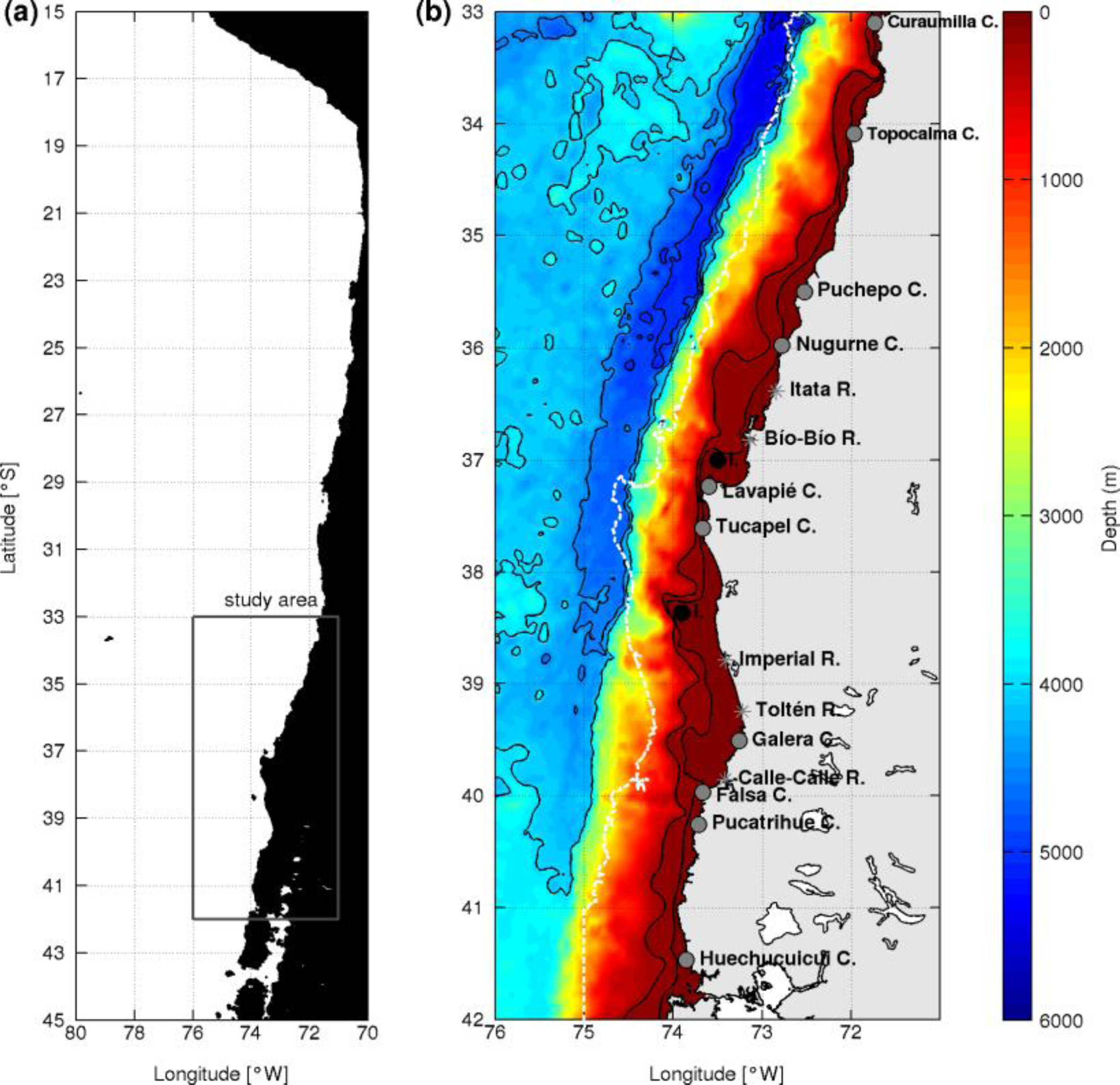
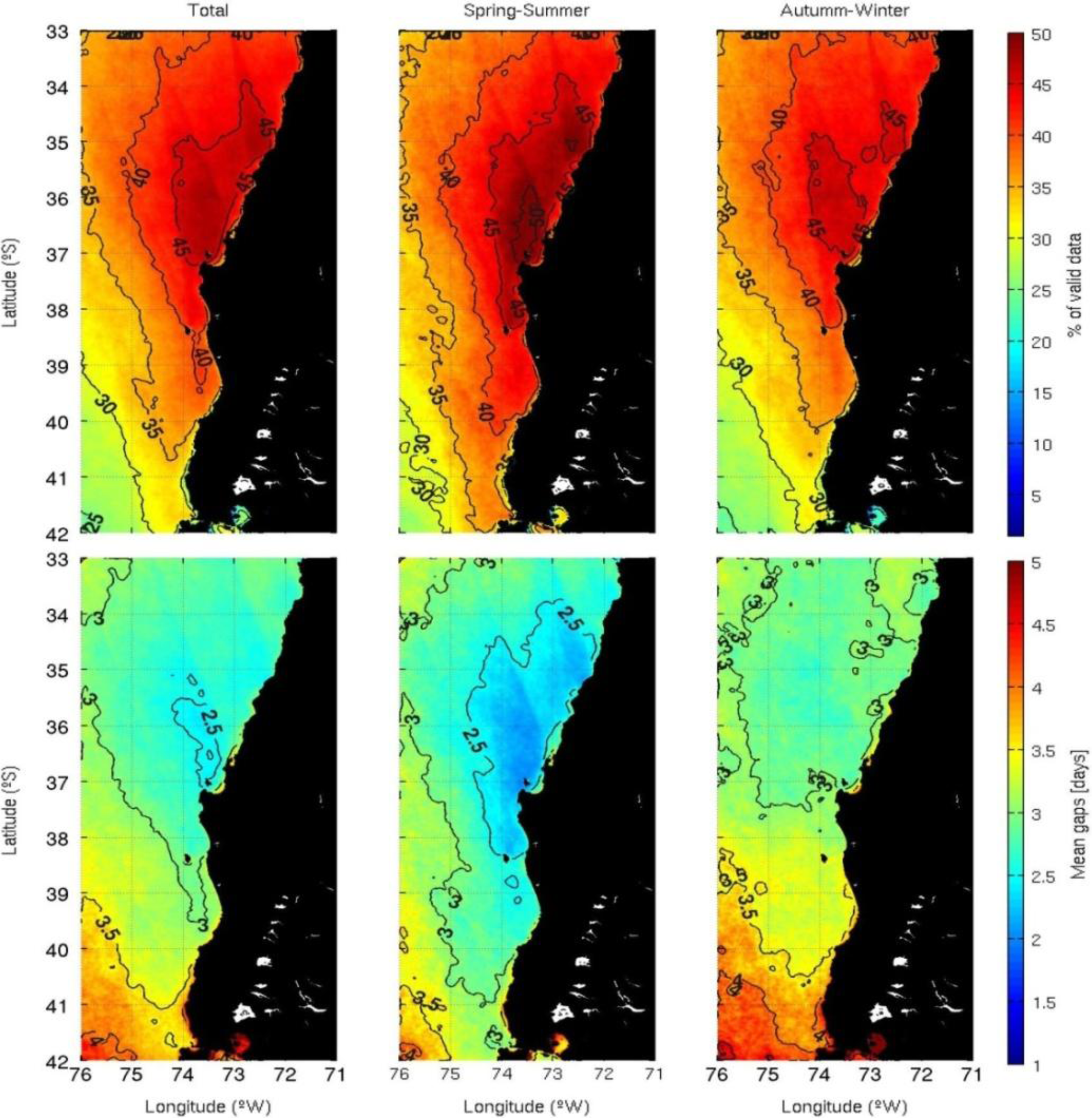
2.1. Satellite Chl-a, SST, Wind and Altimetry Data

Ten years (2002–2012) of satellite data on surface Chl-a, as well as of sea surface temperature (SST), wind (stress and stress curl), and altimetry (sea level and eddy kinetic energy), were analyzed for the region off central-southern Chile (33–42°S, coast to 76°W; Figure 1). Daily data of Chl-a (OC3 algorithm) and SST, with a spatial resolution of ∼1 × 1 km, were obtained from level-2 products of the Moderate Resolution Imaging Spectro-radiometer—MODIS-Aqua mission ( http://oceancolor.gsfc.nasa.gov/). Daily surface wind data, with a spatial resolution of 25 × 25 km, were obtained from the Cross-Calibrated Multi-Platform project (CCMP; product L3.0 for Ocean Surface Wind), which integrates measurements from several missions ( http://podaac.jpl.nasa.gov/). Wind stress (WS) and wind stress curl (WSC) were calculated from these data [27]. Weekly altimetry data (25 × 25 km resolution) come from the merged product of several missions and which is distributed by AVISO ( www.aviso.oceanobs.com); the calculation of eddy kinetic energy (EKE) followed the description in [23]. Chl-a, wind, SST and altimetry data were low-pass filtered (cosine Lanczos with a half amplitude at 8 days) as to remove the synoptic signal and then the data were resampled every 5 days, mostly because of the computing capabilities available to us.

Gaps in the satellite data, caused by cloud coverage, were filled out through interpolation using the objective method DINEOF (Data Interpolating Empirical Orthogonal Function) applied iteratively with a window of 31 d [35]. This method was found to be more adequate than other available alternatives, as it conserves the variance of the time series. In the case of surface Chl-a, the distribution of missing data is shown in Figure 2, expressed in terms of the percentage of valid data (satellite data reported) and mean gap in the data (number of consecutive days with no valid data). First, seasonality (spring-summer and autumn-winter) does not influence the missing data; second, more than 30% of valid data were found for most of the region and the mean gaps between valid data were mostly between 3 and 3.5 days (maximum values were 20–30 days and during the autumn-winter period). In terms of Chl-a data calibration, previous studies have found a reasonable agreement between in situ (fluorometry and HPLC) and satellite estimates [36]. The influence of colored dissolved organic matter (CDOM) on the Chl-a signal has, however, not been investigated yet but it could be important in the most inshore area and embayments due to the discharge of rivers in this region.

2.2. Data Analysis

The main frequencies of spatial and temporal variability of the different variables were evaluated by the Multitaper Method-Singular Value Decomposition (MTM-SVD) method, which combines two techniques developed independently [37]. This method has been described in detail by us [38] and a MATLAB implementation of the algorithms is freely available. In contrast to other methods (e.g., spectral analysis, Orthogonal Empirical Function and the SVD), the MTM-SVD method detects the oscillations that are statistically significant and whose signals are highly correlated in several time-series obtained in the spatial domain and within a particular bandwidth. This method allows a description of the spatial characteristics of the frequencies of interest through a reconstruction process of the time series. In using the MTM-SVD method, the local fractional variance spectra for each of the variables in the time series was first calculated in order to identify the significant frequencies of variability for each of them; the parameters used were those recommended [37] and previously applied by us for the HCS region [10]. The association between Chl-a and physical forcing in the region were assessed through linear correlation analysis using the reconstructed time series obtained with the MTM-SVD method. Lags (in days) were calculated as the difference in the dates of the maximum values in each of the reconstructed cycles.

3. Results and Discussion

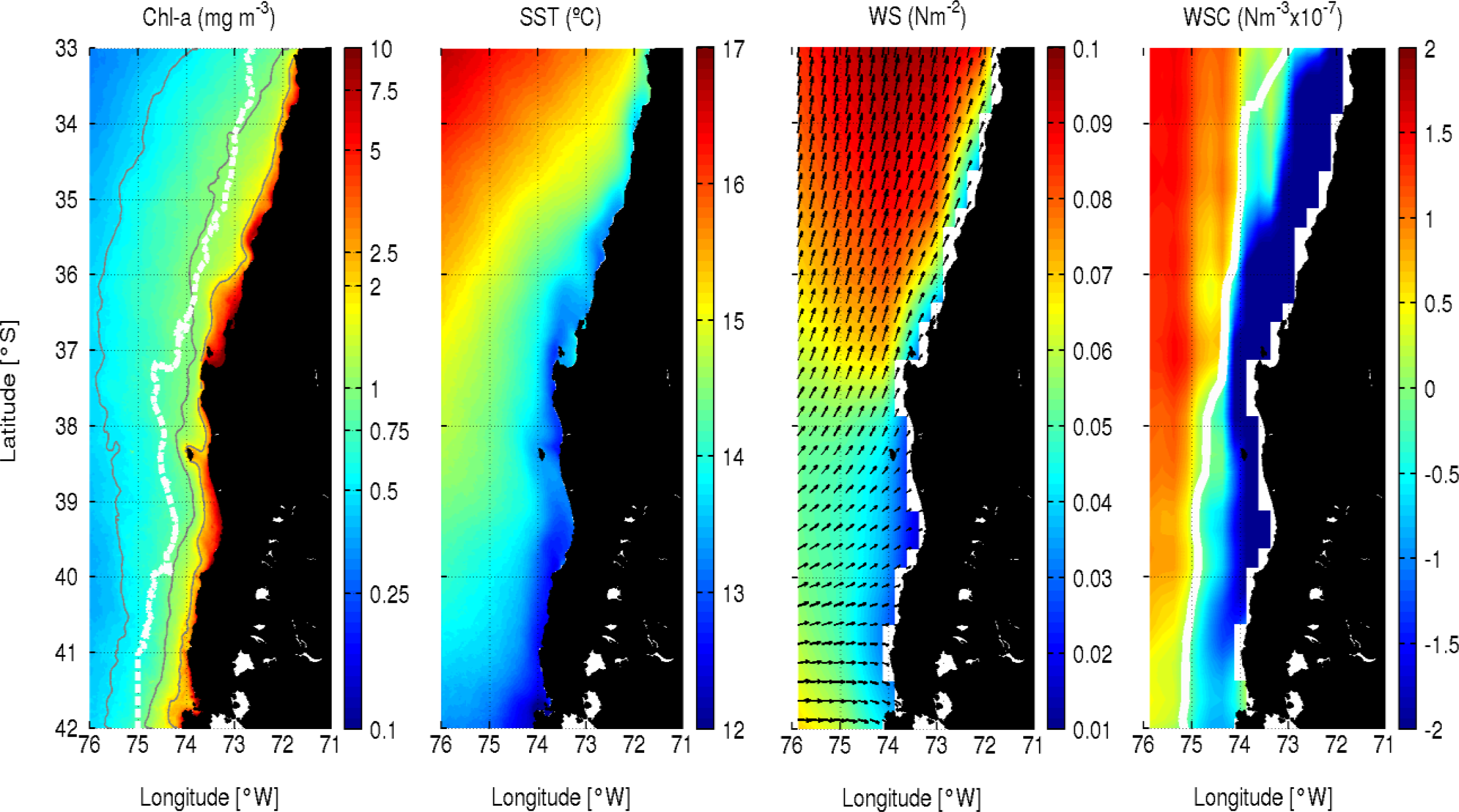
3.1. Mean Distributions of Satellite Chl-a, SST and Winds

The mean distribution of Chl-a concentration in the region off central-southern Chile (∼10 years time series) is represented in Figure 3. A strong cross-shore difference was found between the CUZ (between 0 and 100 km from the coast) and the CTZ (offshore of the CUZ and out to 76°W), with maxima in the former. In the CUZ, the highest mean values (>2 mg·m⁻³) were usually restricted to the inshore (∼20–60 km) whereas farther offshore extensions were located in areas where the shelf was wider (Figure 1), such as the Itata Terrace (∼36–37°S) and between Mocha Island and P. Galera (∼38–40°S). Towards the CTZ, Chl-a values equal to 1 mg·m⁻³ were located between ∼60 and 110 km offshore whereas those of 0.5 mg·m⁻³ stretched out to ∼140 and 280 km offshore. The spatial distribution of these isolines (0.5 and 1 mg·m⁻³) was clearly different in the northern section (33–38°S) compared to the southern section (38–42°S); their cross-shore extensions were about twice as wide in the former.

The general pattern of Chl-a distribution described in this study is consistent with previous satellite-based results using coarser time-space resolution data for the region off central-southern Chile [6,22]. The analyses of SeaWiFS time series data (1998–2005, monthly means) in the region between 33 and 40°S [22] indicated that, albeit the spatial variability found between seasons, the mean offshore location of the Chl-a isoline of 0.5 mg·m⁻³ ranged between ∼100 and 200 km from the coast, further offshore in the area north of P. Lavapié (∼37°S). Furthermore, this study suggested that the Chl-a isoline of 1 mg·m⁻³ represents the offshore limit of the upwelling thermal front; in turn, this isoline is mostly found within the first 100 km of the coast [10]. In the analyses of SeaWiFS time series data (1998–2003, monthly means) for the region between 18 and 40°S [6], the 0.5 mg·m⁻³ isoline was found at ∼200–300 km offshore during that period; however, their indication that the offshore extension of the highest Chl-a values (5 mg·m⁻³) is located ∼200 km from the coast in the region off central-southern Chile is not supported by that or other figures in this publication.

The mean SST distribution during the 2002–2012 time series (Figure 3) displayed cooler waters in the southern section and along the CUZ; also, a strong SST gradient, almost parallel to the coast, was present in the northern section but not in the southern. This pattern of SST distribution is similar to a previous description in [22]. According to these authors, the thermal front was related to upwelling activity and is present most of the year, except in winter. They also associated this front with an equatorward jet which, northwest of P. Lavapié, moves offshore and generates intense mesoscale activity. This jet is stronger in spring-summer and it remains close to the coast (coastal jet) in the southern section (>37°S) but becomes an offshore jet (CTZ jet) in the northern section [29].

The mean distributions of wind direction, WS, and WSC values in the same time series (2002–2012) also showed meridional and zonal variability in the region of study (Figure 3). In the northern section, mean WS is equatorward (favorable to offshore Ekman transport) and more intense whereas it is weaker and mostly eastward (towards the coast and upwelling neutral) in the southern section. In comparison with the region of the California Current System, where the band of transition in the mean direction of WS is located at ∼45°N [15], in the HCS this band is located around 41–42°S. Furthermore, mean WSC is cyclonic (negative) and favorable to upwelling (Ekman pumping) in a band (∼25–70 km width) close to the coast and more intense in the northern section. Immediately offshore of this band, a slightly broader band (∼70–140 km width) contained WSC values of around zero; weak anticyclonic values appeared offshore of it, mostly in the northern section.

Previous studies have shown that the most intense and persistent upwelling activity in this region occurs between 35 and 38°S [26,39]. The abrupt change in coastline orientation north of 37°S could contribute to the differences in WSC between the northern and southern sections; also, shelf width is greatly reduced in the area around 37°S compared to the adjacent regions (Figure 1). These changes in bathymetry and coastline orientation might influence the generation of greater mesoscale activity to the north of P. Lavapié, as suggested by modeling results [40]; observational data also suggest higher mesoscale activity in the area around P. Lavapié and to the north of it [22,41–43]. The observed differences in wind patterns between the northern and southern sections in the region off central-southern Chile coincide with the differences in the offshore extension of Chl-a values (isolines of 0.5 and 1 mg·m⁻³; Figure 3) in these sections.

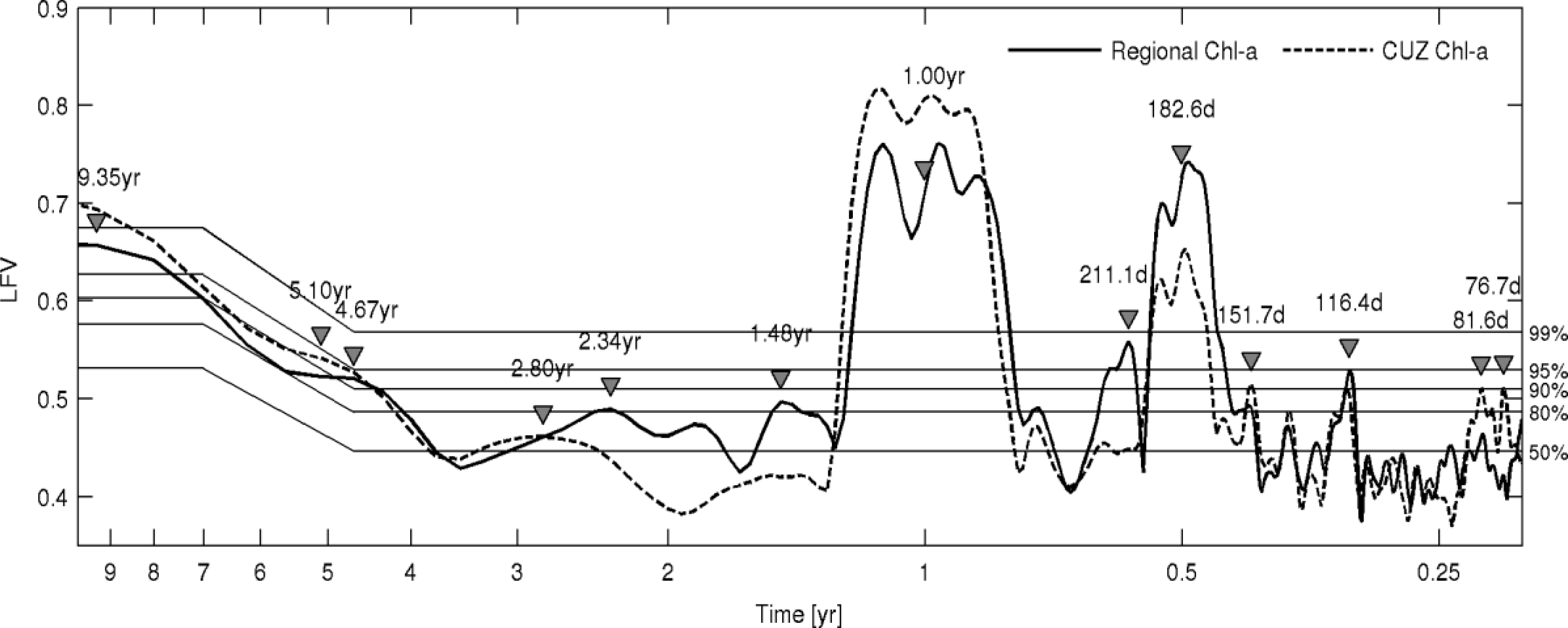
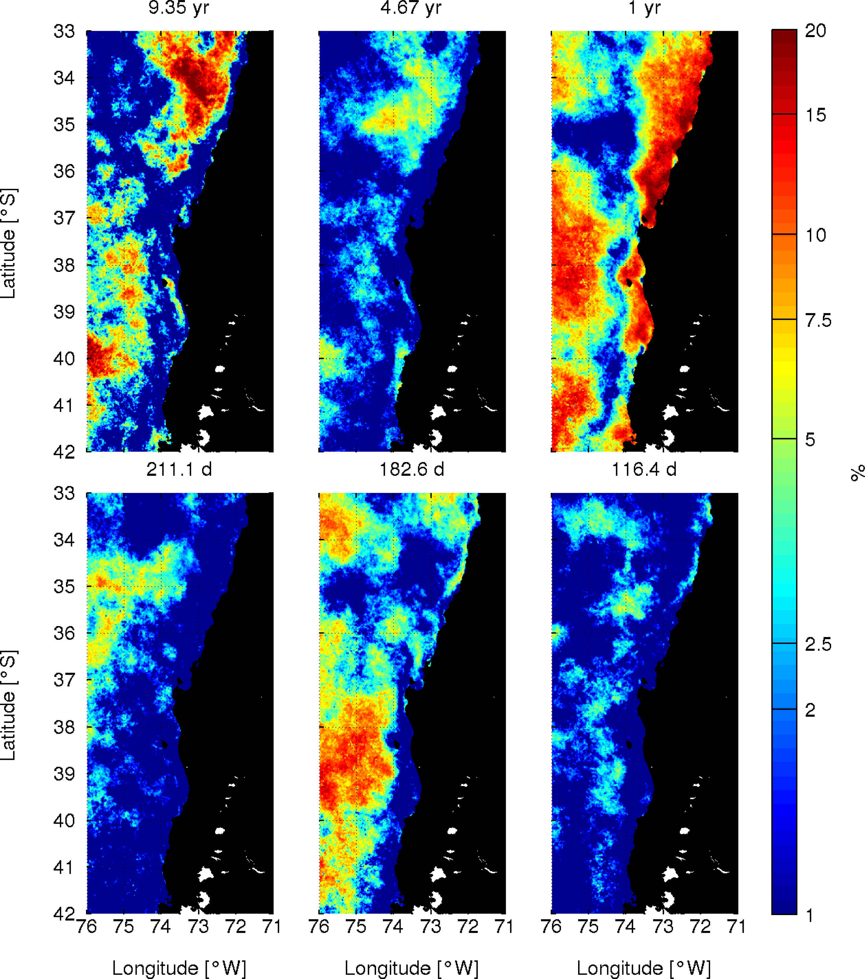
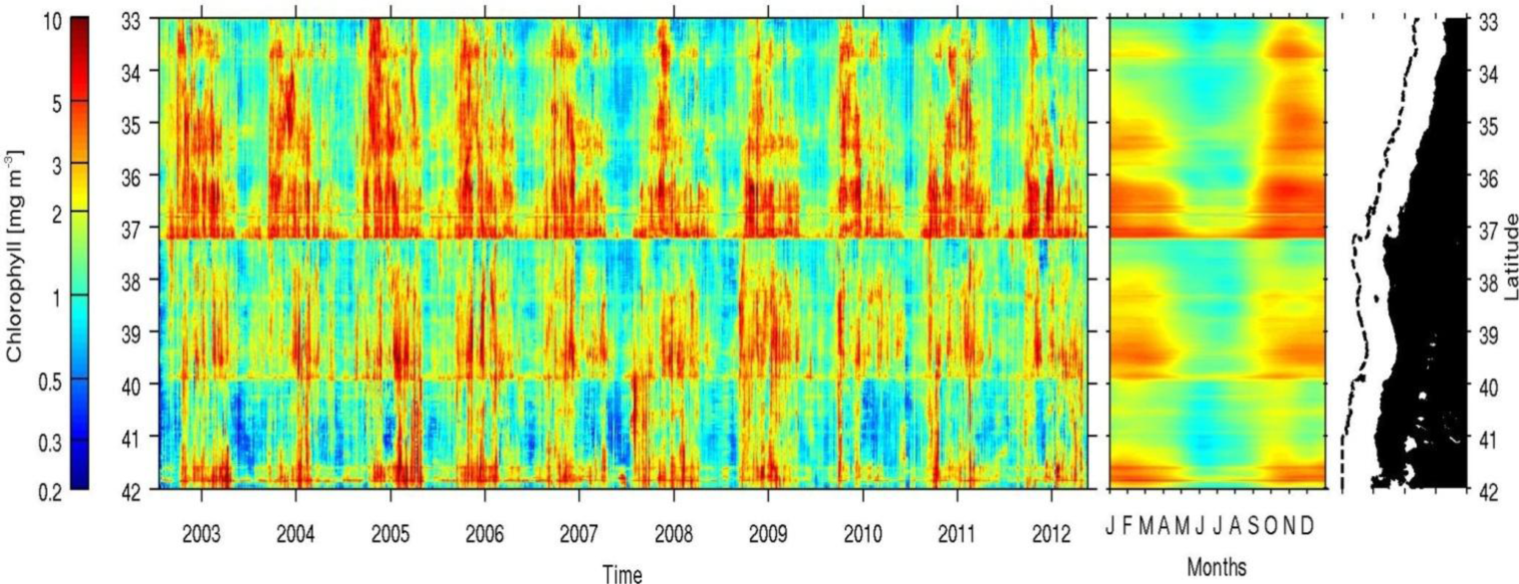
3.2. Time-Space Variability of Chl-a

The dominant frequencies of temporal variability of Chl-a were analyzed and the results are represented in terms of local fractional variance (LFV) spectra (Figure 4). During the ∼10 years’ time series, the dominant frequency of Chl-a variability in the region and in the CUZ was annual (∼1 year), although a semiannual signal (∼180 days) was also highly significant (>99% confidence level). Other intrannual (116 and 211 days) and interannual frequencies (∼5 and 9 years) were also significant but not at the same level (>90%). The annual frequency of Chl-a was spread between 10.5 and 13.5 months, resulting in a ±1.5-month displacement within the time series. This may be related to year-to-year changes in the phenology of phytoplankton biomass, as has been suggested for the region between 35 and 38°S [44]. The variability in Chl-a associated with periods between ∼115 and ∼180 days, has been attributed to mesoscale activity in the region, especially to the passage of mesoscale eddies generated at the shelf break [23]. At the interannual scale, the El Niño Southern Oscillation (ENSO) cycle has been found to explain Chl-a variation in the region [10].

The spatial distribution of Chl-a variance explained in each of the significant LFV frequencies is represented in Figure 5. In the CUZ, the Chl-a variance explained by each of the highest (116, 183, and 211 days) and lowest (4.7 and 9.4 years) frequencies was relatively low (<5%), especially in the southern section. In contrast, the Chl-a variance explained by the annual cycle was higher in most of the CUZ (>10%). In the adjacent CTZ, the variance explained by the annual signal was minimal (<2%) in a band located between ∼100 km (southern section) and 150 km (northern section) from the coast. This band presented a meridional continuity but it varied in width between the northern section (>200 km) and the southern section (∼100 km). Offshore of this band, the variance explained by the annual signal increased again in the CTZ, except in the area between 35 and 36°S (Figure 5).

In terms of the annual cycle of Chl-a, the above patterns of distribution are similar to those previously reported in a study including the region between 18 and 40°S and out to 86°W [6]. This study described the presence of a transitional band (50–200 km wide, depending on latitude) where the annual cycle is weak, located between ∼100 and 170 km of the coast in the region between ∼33 and 38°S. This band coincides with the location of the equatorward jet in the region between 28 and 42°S and its further offshore extension in the northern section matches the progression from a coastal jet to a CTZ jet [29]. This jet is stronger during the spring-summer upwelling season but it is also detectable in autumn [29], as is the associated wind jet [45]. It is likely, then, that the low annual variability of Chl-a in the transitional band is explained, at least in part, by the relatively constant presence of the coastal-CTZ jet in the region of study. In addition, the mean distribution of the 0.5 and 1 mg·m⁻³ Chl-a isolines (Figure 3) coincide with the position reported for this jet [29]. In the California Current System, this band has also been described and it coincides with the path of the current core in the area off northern California [46].

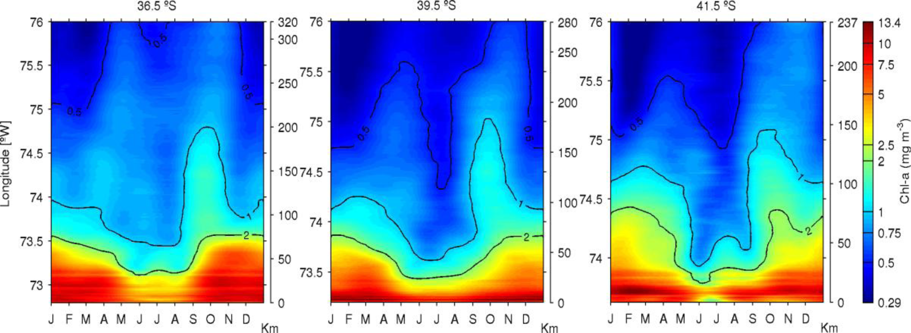
3.3. Time-Space Variability of Chl-a during the Annual Cycle

The time-space distribution of Chl-a in the CUZ, where the highest values are usually concentrated in the region off central-southern Chile, are depicted in Figure 6, together with the mean annual cycle. The annual cycle of Chl-a in the CUZ is characterized by maxima during spring-summer (October to March) and minima during the winter, as has been described in previous studies [6,10,22]. However, this cycle displays alongshore differences within the CUZ; it is quite weak in the areas around main upwelling capes (e.g., at ∼37 and ∼40°S), where low Chl-a concentration are found year-round. Furthermore, higher Chl-a values throughout the year were found in the area of the Gulf of Arauco, located immediately to the north of P. Lavapié (Figure 1). The alongshore discontinuities in Chl-a distribution at ∼37 and ∼40°S divided the CUZ into three distinct areas: ∼33–37°S, 38–40°S, and 41–42°S. Among the latter, maximum Chl-a values (>5 mg·m⁻³) were only found in the northern section, especially between 36 and 37°S. Furthermore, the annual cycle appears to be more extended (∼8 months) around 35–37°S than around 33–35°S. The alongshore differences in coastal Chl-a maxima do not appear to be related to river discharges (and the associated CDOM and particulates) since several rivers are present in the region between 36 and 40°S. On the other hand, the alongshore variations of Chl-a within areas of strong annual signal appear to be related to shelf width (Figure 1), those with a narrower shelf having a weaker amplitude or shorter duration of the positive phase during the annual cycle.

At selected latitudes where high Chl-a concentration persisted year-round (36.5, 39.5, and 41.5°S; from the coast to 76°W), the across-shore distribution of Chl-a during the annual cycle is shown in Figure 7. In the three cases, relatively high Chl-a concentrations (>2 mg·m⁻³) remained present year-round in the inshore area, as previously described for the region between 33 and 40°S [22]; the extent to which this is influenced by CDOM is, however, unknown. Chl-a values >1 mg·m⁻³ were distributed mostly within the first 50 km during the winter and extended out to ∼100 km from the coast during spring-summer but farther offshore in September and October (∼150–200 km offshore). In the CTZ, Chl-a values ∼0.5 mg·m⁻³ reached out to 76°W in the three areas during a longer time (∼6 months) in the northern section (36.5°S) compared to the southern section (2–3 months). The 0.5 mg·m⁻³ isoline was located farther offshore during September and October but also during April–May in the three areas; these months represent the transitions between winter-spring and autumn-winter, respectively.

The offshore extensions of Chl-a had a stationary character in the CUZ but they appear to gradually propagate offshore in the CTZ (∼1 month delay in ∼100 km; Figure 7); the propagation speed (∼3.3 km day⁻¹) is similar to that of mesoscale eddies in this region [41,42]. A similar plot of the mean annual cycle of SST (not shown) did not reveal an association with the Chl-a variations described above. A study on the seasonal variability of mesoscale eddies, in the region between 15 and 38°S and during the 2002–2009 period [43], showed that the maximum number of anticyclonic eddies appear during the autumn (March–May) and the minimum in spring (September–December), in opposite phase with those of cyclonic eddies, with maxima in spring (September–November) and minima in summer-autumn (January–April). This pattern further suggests that the offshore propagations of Chl-a (Figure 7) could be related to the formation of cyclonic and anticyclonic mesoscale eddies in the shelf-break area and their westward displacement in the CTZ. Moreover, mesoscale eddies appear to have a stronger expression in the northern section (north of P. Lavapié) and could explain the meridional change in the extent of the offshore distribution of the mean Chl-a values between 0.5 and 1 mg·m⁻³ (Figure 3).

The spatial reconstruction of the annual cycle of Chl-a variability in the region off central-southern Chile (Figure 8) displayed differences in the alongshore and across-shore directions. In the CTZ, Chl-a positive anomalies start to increase in the northern limit (<35°S) during mid-April (phase 270°), after which they gradually increase in intensity and spread southwards, attaining the southern limit by July (phase 0°). Maximum positive anomalies are attained by mid-July (phase 0°) in the northern limit, early September (phase 45°) in the central zone (36–39°S), and by mid-October (phase 90°) in the southern limit (>40°S). Negative Chl-a anomalies start to appear in the CTZ during mid-October (phase 90°) in the northern limit and they continue to propagate southwards, following the same pattern as the positive anomalies but with minima in opposite phase with respect to the maxima.

In the CUZ, Chl-a positive anomalies start to increase in the northern limit on September (phase 45°), after which they gradually increase in intensity and spread southwards, attaining the southern limit by early December (phase 135°). Maximum positive anomalies are attained in early December in the northern section and mid-January (phase 180°) in the southern section. Negative Chl-a anomalies start to appear in the CUZ during early March (phase 225°) in the northern limit and they continue to propagate southwards, following the same pattern as the positive anomalies but with the minima in opposite phase with respect to the maxima. Overall, when positive (negative) Chl-a anomalies in the CTZ are spread along the whole region, negative (positive) anomalies extend along the CUZ (phases 0 and 180°, respectively); also, the coastal maxima lag ∼3 months the CTZ maxima. Recently, [10] suggested that, in the region between 30 and 40°S, positive Chl-a anomalies during the annual cycle are generated close to the CUZ in March and then undergo a zonal extension until reaching their greatest intensity in the CTZ in July.

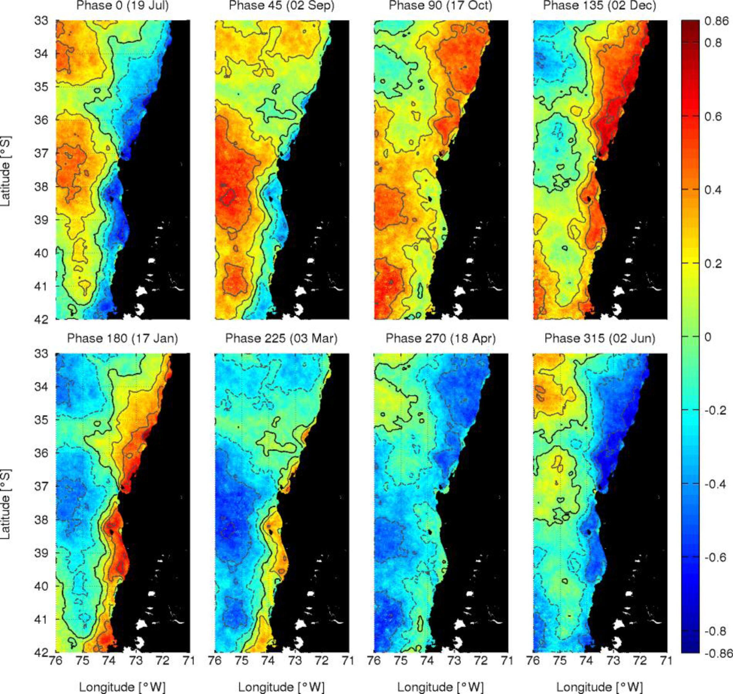
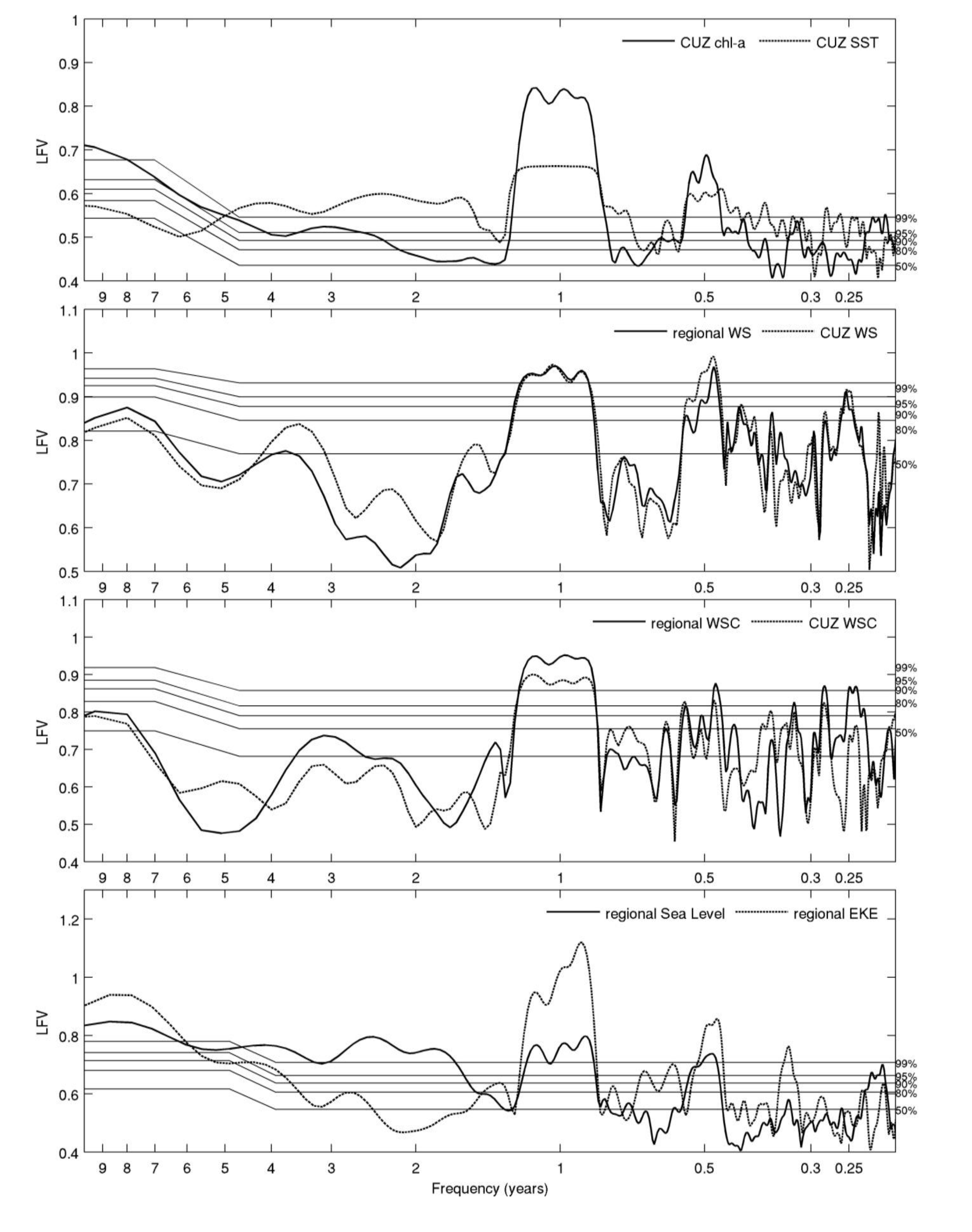
3.4. Annual Chl-a Variability and Its Association with Wind Forcing, SST, Sea Level and EKE

The LFV spectra for Chl-a and SST in the CUZ, and for WS, WSC, sea level and EKE in the region and in the CUZ, displayed similar patterns of variability (Figure 9). The dominant mode of variability is annual in all of them; also, they all (less so for WSC) present a highly significant (>99%) semi-annual signal (∼180 days). The interannual frequencies are not significant for WS and WSC but are so for the rest of the variables. For coastal Chl-a, the signal was significant at ∼3 and 5 years and at the lowest frequency (∼8–9 years), the limit of the time series data; for EKE it was significant only at the lowest frequency whereas for coastal SST and sea level the significant interannual variability was spread over a broad band (from 1.7 to >4 years). Previously, [10] found that most of the Chl-a variance in the interannual frequency (1.4, 1.8, 2.1 and 3.3 years combined) was found in the oceanic zone (20%–25%) and that periods of ∼3.3 years were also significant for WS, sea level anomalies, and EKE. Their times series (1997–2007) included a strong El Niño event (1997–1998) whereas the 2002–2012 time series displays only moderate to weak events (National Center for Atmospheric Research NCAR: https://climatedataguide.ucar.edu/climate-data/multivariate-enso-index).

The spatial distribution of the variance explained by the annual cycle of WS, WSC, sea level, EKE and SST in the region off central-southern Chile is represented in Figure 10. For WS, the highest contribution to the variance was concentrated in the northern section whereas it was minimal in the southern section. For WSC, the highest contribution to the variance appeared in the CUZ (between 34 and 40°S) and in the most offshore section (between 37 and 42°S). Between these two zones, a band of minimum annual variance was present between 74 and 75°W in the 37–42°S section whereas it occupied the whole CTZ in the northern section. This band coincides with the transitional band of low variance in the Chl-a annual cycle described above (Figure 5) and it is associated with the position of the coastal-CTZ jet, where WSC is close to zero (∼75°W). In turn, this coincides with the climatological location of the low-level wind jet, which is characteristic in the region between 30 and 38°S [45,47]. On the other hand, the annual variance in sea level and EKE were mostly constrained to the CTZ, in agreement with the results of [10]. For SST, the variance explained by the annual cycle was relatively high over the study region, with higher percentages in the CTZ compared with the CUZ.

The spatial reconstruction of the annual cycles of WS and WSC are represented in Figure 11; those for sea level and EKE are not shown because of the narrow zonal band considered in this study but they have been previously presented by [10]. In the case of SST, the spatial reconstruction indicated that the signal was stationary, in contrast with the signal for Chl-a (Figure 8), therefore is not included here. The annual cycle of WS anomalies exhibits a dipole (opposite phases) between the northern and southern sections, with a transitional band around 37–38°S. In the northern section, wind direction (annual anomalies + mean field) is mostly towards the north-northeast throughout the year but with very low WS values during winter months (phases 315, 0 and 45°) and maximum in spring-summer (phases 135, 180, and 225°). In the southern section, wind reversal occurs; towards the southeast during phase 0° (mid-July; maximum positive anomalies) and towards the northeast during phase 180° (mid-January), with transition periods in mid-October and mid-April (phases 90 and 270°, respectively).

These wind patterns coincide with those shown in [22]. The meridional WS (1999–2007 time series from QuikSCAT) in the 34–37°S section are mostly upwelling favorable throughout the year but close to zero values during the winter (May to August). Similarly, [48] used QuikSCAT winds (2000–2007) for the region between 8 and 38°S to obtain the seasonal climatology; WS was weaker and mostly towards the coast during autumn-winter at ∼37–38°S and upwelling favorable during the year in the area to the north but weaker during autumn-winter months. Results from [28] also coincide with the above, using QuikSCAT data (2000–2005) in the region between 5 and 45°S to obtain summer and winter climatologies.

In the reconstruction of the annual cycle of WSC (Figure 11), the northern and southern sections also display differences. In the northern section, the values are always negative in the CUZ but they are weaker and mostly inshore during mid-July (phase 0°); after this, they spread to the west and are more intense, reaching a maximum from the beginning of December (phase 135°) to mid-January (phase 180°). This pattern coincides with that of WS anomalies in this section, with weaker (stronger) WSC anomalies associated with maximum negative (positive) WS anomalies. In the southern section, WSC anomalies are negative in the CUZ and attain a maximum offshore extension from mid-January (phase 180°) to the beginning of March (phase 225°). In this case, weaker (stronger) WSC anomalies coincide with the maximum positive (negative) WS anomalies. In the CTZ, positive anomalies appear in the most offshore zone of the northern limit in mid-July (phase 0°) and they gradually extend southwards, dominating the whole CTZ (west of 75°W) from the beginning of December (phase 135°) to mid-January (phase 180°).

Upwelling favorable winds in the region of central-southern Chile are associated with the south-eastern Pacific Subtropical Anticyclone, which has a meridional migration during the annual cycle. In the southern section, winds are associated with the northern border of the West Wind Drift, the position of which also changes during the annual cycle [26]. Maximum WS favorable to upwelling in the CUZ is distributed northward of ∼38–40°S during the spring-summer and northward of ∼33°S during the autumn-winter [28,48]. Maximum WSC favorable to upwelling displays a similar pattern of distribution, with the band of negative values in the CUZ located farther south in summer in comparison with winter [28]. In addition, it is likely that a relatively higher EKE activity develops in the northern section in response to the sharp change in coastline orientation at P. Lavapié (eastward bend), especially during the period of upwelling favorable winds. This effect has been described before for the study region, using numerical models [40].

The associations between Chl-a and wind forcing, Chl-a and sea level, and Chl-a and EKE for the annual frequency (top panels), and of the lag time (days) between the Chl-a annual maxima and the annual maxima of these variables (bottom panels), are represented in Figure 12. Annual increases of Chl-a and WS are positively correlated in the northern section of the CUZ (r = 0.4 to 0.8) but its association progressively diminishes westward until ∼74°W, after which they turned negative in the CTZ (r = −0.8). In this section, Chl-a increases were mostly in phase with those in WS favorable to upwelling (∼10 days) but they progressively lag behind WS increases (from −10 to −60 days) towards offshore. In the southern section, the correlations are mostly negative, especially in the CUZ (r = −0.8); the fluctuations in Chl-a are offset behind those of WS (from −90 to −180 days). A negative coefficient and the observed offset can be explained by a seasonal reversal in mean wind direction in this section, the annual maximum in WS (Figure 11; phases 315, 0, and 45°) being unfavorable to upwelling and associated with negative Chl-a anomalies in the CUZ (Figure 8). These results suggest that the annual increase in WS favorable to upwelling is a potential forcing of the annual increase in Chl-a along the CUZ (33–42°S), despite the differences in the patterns of WS anomalies between the northern and southern section (Figure 11). This is not the case, however, for the CTZ, where winds are upwelling favorable when Chl-a anomalies are minimal (Figures 8 and 11).

The correlations between Chl-a and WSC (Figure 12) are negative (r = −0.6 to −0.8) along the CUZ and positive (r = 0.4 to 0.8) in a band (∼100 km width) immediately offshore of it (∼74–75°W). In the CUZ, negative WSC values (favorable to upwelling) are strongly correlated with positive Chl-a anomalies and there is an offset of ∼120–180 days. This result suggests that WS and WSC are both potentially relevant drivers of the annual Chl-a increase (decrease) in the coastal zone, as has been suggested for the Southern California Current System [49] and off Peru [50]. In the offshore band, the highest correlations occur in the area where the mean WSC is almost neutral (Figure 3) and where the annual cycle of Chl-a displayed low variability (Figure 7). Lag time in this case is highly variable and could not be clearly related to a specific physical process, except that this band represents a transition between the CUZ and the CTZ.

The spatial distribution of the correlations between Chl-a and sea level and between Chl-a and EKE are very similar (Figure 12), mostly negative except in some areas where they are positive (0.4 to 0.8). The latter are concentrated in a band where mesoscale eddies are frequently formed (around the shelf-break) in the northern section, in agreement with previous results [42]. In the CUZ, maximum anomalies in Chl-a (Figure 8) correspond with negative anomalies in sea level and EKE during the annual cycle (data not shown). The band of positive values has a similar position as that for the correlations between Chl-a and WSC and also with that of a coastal-CTZ jet [29]. Its distinctiveness in the northern section is probably the result of higher mesoscale activity compared to the southern section, associated with the influence of a very prominent cape (P. Lavapié) and a change in coastline orientation to the north of it. Chl-a and SST correlations (Figure 12) were mostly positive in the CUZ but the annual increase in SST lag behind that in Chl-a by ∼30 to ∼90 days (increasing towards offshore), implying that SST is not an influencing factor. In the CTZ, these correlations are negative (inverse annual cycles) and SST lag behind Chl-a by ∼120–150 days. This lag might be linked to a covariation in Chl-a and SST in connection with the effects of internal waves (e.g., Rossby waves), where a positive (negative) phase of the wave will involve a deepening (shallowing) of the thermocline together with an increase (decrease) in SST and a decrease (increase) in Chl-a [51].

4. Conclusions

About a decade of satellite Chl-a, SST, wind, and sea level were used to analyze the time-space variability of phytoplankton biomass in the region off central-southern Chile (33–42°S).The annual cycle of Chl-a was dominant in the CUZ and the CTZ (in different phases), except in a transitional band between them; this band coincides with the location of a coastal-CTZ jet. The annual cycle of Chl-a displayed strong alongshore variation and, in association with the annual cycle of winds, two distinct sections were identified. In the northern section (33–38°S), the climatological mean Chl-a values were higher in the coastal band and the 0.5 mg·m⁻³ isoline extended out to 200 km of the coast. In this section, mean wind forcing (WS and WSC) was favorable to upwelling year-round but weak during the autumn-winter period. In the southern section (38–42°), annual wind reversal was characteristic, with upwelling favorable winds dominating from December to April but WS and WSC were weaker than in the northern section. Chl-a changes in the CUZ were positively (negatively) associated with WS in the northern (southern) section, and negatively with WSC. In the CTZ, the variations in Chl-a were not so clearly explained by wind forcing, sea level, or EKE except in the area of the shelf-break, where mesoscale eddies are frequently formed. The observed time-space differences in the distribution of Chl-a are critical in the understanding of the processes that control Chl-a variability within the region and in the identification of the potential impacts of ongoing climate change on phytoplankton biomass in coastal upwelling regions.

References

1. Hill, A.E.; Hickey, B.M.; Shillington, F.A.; Strub, P.T.; Brink, K.H.; Barton, E.D.; Thomas, A.C. Eastern Ocean Boundaries. In The Sea; Robinson, A.R., Brink, K.H., Eds.; John Wiley and Sons: New York, NY, USA, 1998; Volume 11, pp. 29–67. [Google Scholar]
2. Mackas, D.L.; Strub, P.T.; Thomas, A.; Montecino, V. Eastern Regional Ocean Boundaries-Pan Regional Overview. In The Global Coastal Ocean: Interdisciplinary Regional Studies and Syntheses—Pan-Regional Syntheses and the Coasts of North and South America and Asia, the Sea; Robinson, A.R., Brink, K., Eds.; Harvard University Press: Cambridge, MA, USA, 2006; Volume 14, pp. 21–60. [Google Scholar]
3. Chavez, F.P.; Messié, M. A comparison of eastern boundary upwelling systems. Prog. Oceanogr 2009, 83, 80–96. [Google Scholar]
4. Thomas, A.C.; Strub, P.T.; Weatherbee, R.A.; James, C. Satellite views of Pacific chlorophyll variability: Comparisons to physical variability, local versus nonlocal influences and links to climate indices. Deep Sea Res. Part II 2012, 77–80, 99–116. [Google Scholar]
5. Thomas, A.C.; Carr, M.E.; Strub, P.T. Chlorophyll variability in eastern boundary currents. Geophys. Res. Lett 2001, 28, 3421–3424. [Google Scholar]
6. Yuras, G.; Ulloa, O.; Hormazabal, S. On the annual cycle of coastal and open ocean satellite chlorophyll off Chile (18–40°S). Geophys. Res. Lett 2005. [Google Scholar] [CrossRef]
7. Lauthuilière, C.; Echevin, V.; Lévy, M. Seasonal and intraseasonal surface chlorophyll-a variability along the northwest African coast. J. Geophys. Res 2008. [Google Scholar] [CrossRef]
8. Echevin, V.; Aumont, O.; Ledesma, J.; Flores, G. The seasonal cycle of surface chlorophyll in the Peruvian upwelling system: A modelling study. Prog. Oceanogr 2008, 79, 167–176. [Google Scholar]
9. Checkley, D.M.; Barth, J.A. Patterns and processes in the California Current System. Prog. Oceanogr 2009, 83, 49–64. [Google Scholar]
10. Correa-Ramirez, M.A.; Hormazabal, S.; Morales, C.E. Spatial patterns of annual and interannual surface chlorophyll-a variability in the Peru–Chile Current System. Prog. Oceanogr 2012, 92, 8–17. [Google Scholar]
11. Lachkar, Z.; Gruber, N.A. Comparative study of biological production in eastern boundary upwelling systems using an artificial neural network. Biogeosciences 2012, 9, 293–308. [Google Scholar]
12. Carr, M.E.; Kearns, D.J. Production regimes in four eastern boundary current systems. Deep Sea Res. Part II 2003, 50, 3199–3221. [Google Scholar]
13. Henson, S.A.; Thomas, A.C. Phytoplankton scales of variability in the California Current System: Interannual and cross-shelf variability. J. Geophys. Res 2007, 112. [Google Scholar] [CrossRef]
14. Kudela, R.; Banas, N.; Barth, J.; Frame, E.; Jay, D.; Largier, J.; Lessard, E.; Peterson, T.; VanderWoude, A. New insights into the controls and mechanisms of plankton productivity in coastal upwelling waters of the northern California Current System. Oceanography 2008, 21, 40–54. [Google Scholar]
15. Venegas, R.M.; Strub, P.T.; Beier, E.; Letelier, R.; Thomas, A.C.; Cowles, T.; James, C.; Soto-Mardones, L.; Cabrera, C. Satellite-derived variability in chlorophyll, wind stress, sea surface height, and temperature in the northern California Current System. J. Geophys. Res 2008. [Google Scholar] [CrossRef]
16. Weeks, S.J.; Barlow, R.; Roy, C.; Shillington, F.A. Remotely sensed variability of temperature and chlorophyll in the southern Benguela: Upwelling frequency and phytoplankton response. Afr. J. Mar. Sci 2006, 28, 493–509. [Google Scholar]
17. Thomas, A.C.; Brickley, P.; Weatherbee, R. Interannual variability in chlorophyll concentrations in the Humboldt and California Current Systems. Prog. Oceanogr 2009, 83, 386–392. [Google Scholar]
18. Tweddle, J.F.; Strutton, P.G.; Foley, D.G.; O’Higgins, L.; Wood, A.M.; Scott, B.; Everroad, R.C.; Peterson, W.T.; Cannon, D.; Hunter, M.; et al. Relationships among upwelling, phytoplankton blooms, and phycotoxins in coastal Oregon shellfish. Mar. Ecol. Prog. Ser 2010, 405, 131–145. [Google Scholar]
19. Espinosa-Carreon, T.L.; Strub, P.T.; Beier, E.; Ocampo-Torres, F.; Gaxiola-Castro, G. Seasonal and interannual variability of satellite-derived chlorophyll pigment, surface height, and temperature off Baja California. J. Geophys. Res 2004, 109. [Google Scholar] [CrossRef]
20. Lachkar, Z.; Gruber, N. What controls biological production in coastal upwelling systems? Insights from a comparative modeling study. Biogeosciences 2011, 8, 2961–2976. [Google Scholar]
21. Thomas, A.C.; Huang, F.; Strub, P.T.; James, C. Comparison of the seasonal and interannual variability of phytoplankton pigment concentrations in the Peru and California Current Systems. J. Geophys. Res 1994, 99, 7355–7370. [Google Scholar]
22. Letelier, J.; Pizarro, O.; Nuñez, S. Seasonal variability of coastal upwelling and the upwelling front off central Chile. J. Geophys. Res 2009. [Google Scholar] [CrossRef]
23. Hormazabal, S.; Shaffer, G.; Leth, O. The coastal transition zone off Chile. J. Geophys. Res 2004. [Google Scholar] [CrossRef]
24. Sobarzo, M.; Bravo, L.; Donoso, L.; Garcés-Vargas, J.; Schneider, W. Coastal upwelling and seasonal cycles that influence the water column over the continental shelf off central Chile. Prog. Oceanogr 2007, 75, 363–382. [Google Scholar]
25. Silva, N.; Rojas, N.; Fedele, A. Water masses in the Humboldt Current System: Properties, distribution, and the nitrate deficit as a chemical water mass tracer for Equatorial Subsurface Water off Chile. Deep Sea Res. Part II 2009, 56, 1004–1020. [Google Scholar]
26. Strub, P.; Mesías, J.; Montecino, V.; Ruttlant, J. Coastal Ocean Circulation off Western South America. In The Sea; Robinson, A., Brink, K., Eds.; John Wiley and Sons, Inc: New York, NY, USA, 1998; Volume 11, pp. 273–313. [Google Scholar]
27. Bakun, A.; Nelson, C.S. The seasonal cycle of wind stress curl in sub-tropical boundary current regions. J. Phys. Oceanogr 1991, 21, 1815–1834. [Google Scholar]
28. Fuenzalida, R.; Schneider, W.; Garcés-Vargas, J.; Bravo, L. Satellite altimetry data reveal jet-like dynamics of the Humboldt Current. J. Geophys. Res 2008. [Google Scholar] [CrossRef]
29. Aguirre, C.; Pizarro, O.; Strub, P.T.; Garreaud, R.; Barth, J.A. Seasonal dynamics of the near-surface alongshore flow off central Chile. J. Geophys. Res 2012. [Google Scholar] [CrossRef]
30. Anabalón, V.; Morales, C.E.; Escribano, H.R.; Varas, M.A. The contribution of nano- and micro-planktonic assemblages in the surface layer (0–30 m) under different hydrographic conditions in the upwelling area off Concepción, central Chile. Prog. Oceanogr 2007, 75, 396–414. [Google Scholar]
31. Morales, C.E.; González, H.E.; Hormazabal, S.E.; Yuras, G.; Letelier, J.; Castro, L.R. The distribution of chlorophyll-a and dominant planktonic components in the coastal transition zone off Concepción, central Chile, during different oceanographic conditions. Prog. Oceanogr 2007, 75, 452–469. [Google Scholar]
32. González, H.E.; Menschel, E.; Aparicio, C.; Barría, C. Spatial and temporal variability of microplankton and detritus, and their export to the shelf sediments in the upwelling area off Concepción, Chile (∼36°S), during 2002–2005. Prog. Oceanogr 2007, 75, 435–451. [Google Scholar]
33. Böttjer, D.; Morales, C.E. Nanoplanktonic assemblages in the upwelling area off Concepción (36°S), central Chile: Abundance, biomass, and grazing potential during the annual cycle. Prog. Oceanogr 2007, 75, 415–434. [Google Scholar]
34. Morales, C.E.; Anabalón, V.S. Phytoplankton biomass and microbial abundances during the spring upwelling season in the coastal area off Concepción, central-southern Chile: Variability around a time series station. Prog. Oceanogr 2012, 83, 80–96. [Google Scholar]
35. Alvera-Azcárate, A.; Barth, A.; Beckers, J.M.; Weisberg, R.H. Multivariate reconstruction of missing data in sea surface temperature, chlorophyll, and wind satellite fields. J. Geophys. Res 2007, 112. [Google Scholar] [CrossRef]
36. Stuart, V.; Ulloa, O.; Alarcon, G.; Sathyendranath, S.; Major, H.; Head, E.J.; Platt, T. Bio-optical characteristics of phytoplankton populations in the upwelling system off the coast of Chile. Rev. Chil. Hist. Nat 2004, 77, 87–105. [Google Scholar]
37. Mann, M.E.; Park, J. Oscillatory spatiotemporal signal detection in climate studies: A multiple-taper spectral domain approach. Adv. Geophys 1999, 41, 1–131. [Google Scholar]
38. Correa-Ramirez, M.A.; Hormazabal, S. MultiTaper Method-Singular Value Decomposition (MTM-SVD): Variabilidad espacio-frecuencia de las fluctuaciones del nivel del mar en el Pacífico suroriental. Lat. Am. J. Aquat. Res 2012, 40, 1039–1060. [Google Scholar]
39. Atkinson, L.P.; Valle-Levinson, A.; Figueroa, D.; de Pol-Holz, R.; Gallardo, V.A.; Schneider, W.; Blanco, J.L.; Schmidt, M. Oceanographic observations in Chilean coastal waters between Valdivia and Concepcion. J. Geophys. Res. 2002. [Google Scholar] [CrossRef]
40. Leth, O.; Middleton, J.F. A mechanism for enhanced upwelling off central Chile: Eddy advection. J. Geophys. Res 2004. [Google Scholar] [CrossRef]
41. Morales, C.E.; Hormazabal, S.; Correa-Ramirez, M.; Pizarro, O.; Silva, N.; Fernandez, C.; Anabalón, V.; Torreblanca, M.L. Mesoscale variability and nutrient–phytoplankton distributions off central-southern Chile during the upwelling season: The influence of mesoscale eddies. Prog. Oceanogr 2012, 104, 17–29. [Google Scholar]
42. Hormazabal, S.; Combes, V.; Morales, C.E.; Correa-Ramirez, M.; di Lorenzo, E; Nuñez, S. Intrathermocline eddies in the coastal transition zone off central Chile (31–41°S). J. Geophys. Res 2013, 118, 1–11. [Google Scholar]
43. Letelier, J. Surgencia y Estructuras de Mesoescala Frente a Chile (18–42°S). 2010. [Google Scholar]
44. Gomez, F.; Montecinos, A.; Hormazabal, S.; Cubillos, L.A.; Correa-Ramirez, M.A.; Chavez, F.P. Impact of spring upwelling variability off southern-central Chile on common sardine (Strangomera bentincki) recruitment. Fish. Oceanogr 2012, 21, 405–414. [Google Scholar]
45. Garreaud, R.; Munoz, R. The low-level jet off the subtropical west coast of South America: Structure and variability. Mon. Wea. Rev 2005, 133, 2246–2261. [Google Scholar]
46. Legaard, K.R.; Thomas, A.C. Spatial patterns in seasonal and interannual variability of chlorophyll and sea surface temperature in the California Current. J. Geophys. Res 2006. [Google Scholar] [CrossRef]
47. Renault, L.; Dewitte, B.; Falvey, M.; Garreaud, R.; Echevin, V.; Bonjean, F. Impact of atmospheric coastal jet off central Chile on sea surface temperature from satellite observations (2000–2007). J. Geophys. Res 2009. [Google Scholar] [CrossRef]
48. Putrasahan, D.A.; Millar, A.J.; Seo, H. Regional coupled ocean-atmosphere downscaling in the Southeast Pacific: Impacts on upwelling, mesoscale air-sea fluxes and ocean eddies. Ocean Dyn 2013, 63, 463–488. [Google Scholar]
49. Macías, D.; Franks, P.J.S.; Ohman, M.D.; Landry, M.R. Modeling the effects of coastal wind- and wind-stress curl-driven upwelling on plankton dynamics in the Southern Califonia Current System. J. Mar. Syst 2012, 94, 107–119. [Google Scholar]
50. Albert, A.; Echevin, V.; Lévy, M.; Aumont, O. Impact of nearshore wind stress curl on coastal circulation and primary productivity in the Peru upwelling system. J. Geophys. Res 2010. [Google Scholar] [CrossRef]
51. Cipollini, P.; Cromwell, D.; Challenor, P.G.; Raffaglio, S. Rossby waves detected in global ocean colour data. Geophys. Res. Lett. 2001. [Google Scholar] [CrossRef]
Figure 1. The eastern South Pacific Ocean off Peru-Chile (a) and the region of study off central-southern Chile (b), including bathymetry (m) and location of capes (C), rivers (R), and islands (I, marked by black dots). The white dotted-line represents the offshore limit of the first 100 km from the coast, here defined as the Coastal Upwelling Zone (CUZ); offshore of it, the Coastal Transition Zone (CTZ) is found.
Remotesensing 05 05550f1
Figure 2. Distribution of missing satellite Chl-a data (MODIS) during the 2002–2012 time series in the region off central-southern Chile: percentage of valid data (top panels) and the mean gaps (number of consecutive days without data; bottom panels) in the data sets for the total time series and for the spring-summer and autumn-winter periods.
Remotesensing 05 05550f2
Figure 3. Temporal mean distribution of satellite data (2002–2012) in the region off central-southern Chile: Chl-a, SST, WS and WSC. For Chl-a, the black lines represent the 5, 1 and 0.5 mg·m−3 isolines (from the coast to the offshore, respectively) and the white-dotted line indicates the offshore limit of the CUZ. For WS, the arrows indicate mean wind direction and intensity and for WSC the white line represents the zero values.
Remotesensing 05 05550f3
Figure 4. Temporal variability of Chl-a off central-southern Chile: local fractional variance (LFV) spectra for regional (continuous line) and CUZ (dotted line) Chl-a values. Right axis: confidence levels (%).
Remotesensing 05 05550f4
Figure 5. Percentage of explained variance (%) for Chl-a in each of the significant frequency bands in Figure 4 (regional): 9.35 and 4.67 years, and 1 year (top panels); 211.1, 182.6, and 116.4 days (bottom panels). The color scale is logarithmic; the percentages represent only a single maximum value in each peak and not the whole width of it (see Figure 4).
Remotesensing 05 05550f5
Figure 6. Time-space distribution of Chl-a in the CUZ (2002–2012) off central-southern Chile: time-latitude Hovmoller diagram (left panel) and latitudinal distribution of the climatological annual cycle (right panel). The black-dotted line in the right panel represents the offshore limit of the CUZ.
Remotesensing 05 05550f6
Figure 7. Climatological annual cycle of Chl-a at selected latitudes off central-southern Chile: 36.5, 39.5 and 41.5°S, from the coasts to 76°W. Distance from the coast (km) is shown on the right axes.
Remotesensing 05 05550f7
Figure 8. Spatial and temporal (phase) representation of the annual cycle of Chl-a in the region off central-southern Chile. Chl-a anomalies (mg·m−3): positive (continuous lines) and negative (dotted lines) values; the heavier continuous black line is zero. Dates representing each phase are shown in parenthesis (day and month).
Remotesensing 05 05550f8
Figure 9. LFV spectra for the variables in the region off central-southern Chile: Chl-a and SST in the CUZ (top panel), WS and WSC in the CUZ and in the region (central panels), and sea level and EKE in the region (bottom panel). Right axis: confidence levels (%).
Remotesensing 05 05550f9
Figure 10. Percentage (%) of the variance explained by the annual cycle of wind stress, wind stress curl, sea level, EKE and STT in the region off central-southern Chile.
Remotesensing 05 05550f10
Figure 11. Spatial and temporal (phase) representation of the annual cycle of WS and WSC in the region off central-southern Chile. For WS, the color bar represents anomalies in amplitude (N·m−2) and the gray arrows the mean WS field plus the vector anomalies; WSC anomalies plus the mean WSC field (N·m−3 × 10⁻⁷) are represented by the continuous (zero and positive values) and dotted (negative) black lines. Dates for each phase are shown in parenthesis (day and month).
Remotesensing 05 05550f11
Figure 12. Associations between Chl-a and physical variables for the annual frequency. (Top panels): correlation maps between Chl-a and the variables WS, WSC, sea level, EKE and SST, using data derived from the MTM-SVD reconstructions of the annual frequency. (Bottom panels): lag time (days) between the annual maxima in Chl-a and that of each of the other variables with which correlation analyses were performed. All correlations were significant over the 95% confidence level.
Remotesensing 05 05550f12