Article

Optimizing Satellite-Based Precipitation Estimation for Nowcasting of Rainfall and Flash Flood Events over the South African Domain

by
Estelle De Coning
South African Weather Service, Private Bag X097, Pretoria 001, South Africa
Remote Sens. 2013, 5(11), 5702-5724; https://doi.org/10.3390/rs5115702
Submission received: 16 August 2013 / Revised: 18 October 2013 / Accepted: 21 October 2013 / Published: 4 November 2013
(This article belongs to the Special Issue Hydrological Remote Sensing)

Abstract

:
The South African Weather Service is mandated to issue warnings of hazardous weather events, including those related to heavy precipitation, in order to safeguard life and property. Flooding and flash flood events are common in South Africa. Frequent updates and real-time availability of precipitation data are crucial to support hydrometeorological warning services. Satellite rainfall estimation provides a very important data source for flash flood guidance systems as well as nowcasting of precipitation events for the data sparse regions of the African continent. Although low earth orbiting satellites with microwave instruments provide good quality rainfall estimates, their temporal and spatial resolution are not adequate for time-critical services. Precipitation estimation using geostationary satellites is less accurate, but provides excellent spatial coverage, is updated frequently and is available in real-time. This study compares different ways to use and combine satellite precipitation estimates and numerical weather prediction model fields over the South African domain in order to determine the optimal estimate of precipitation, which can also be applied in real-time to support flash flood guidance.

Graphical Abstract

1. Introduction

Global measurements of precipitation are essential to the manage water resources and understand the global climate and hydrological cycle [1]. Rain gauges provide a relatively good direct measurement of rainfall at a specific point. The availability of rain gauge data at a sufficient spatial resolution and close to real-time is limited, especially in data sparse regions such as Africa. However, rain gauges are also prone to measurement errors (such as wind effects) and a point measurement is not always representative of the environment [2]. Although radar systems can provide a valuable indirect measurement of rainfall, this remotely sensed data source also has limitations; its accuracy deteriorates with range from the radar and interference due to clutter, beam blockage and anomalous propagation have to be accounted for. The main advantages of satellite rainfall estimates are the high spatial resolution and coverage over regions where other sources of rainfall data are often not available (oceans, mountains, sparsely populated areas). Remotely sensed rainfall derived from satellite data can provide valuable information for identifying hazardous situations, such as heavy rainfall, that could result in flash floods—even in areas without rain gauges and/or radar systems [3].
Satellite rainfall can be derived from low earth orbiting (LEO) or geostationary satellites (GEO). The LEO satellites have the advantage of high spatial resolution, but the disadvantage is that the spatial coverage is in the form of narrow swaths at times that do not always coincide with precipitating weather systems. These satellites are thus not useful for operational forecasting purposes, although the data can be utilized for other purposes, including data assimilation for numerical weather prediction (NWP). The main advantage of LEO satellites is that the microwave sensors carried by these low orbiting satellites have a more direct link to precipitation than the instruments on board GEO satellites. GEO are located much higher above the earth surface than the LEO satellites and thus have a coarser resolution. However, they have the major advantage that the data and images are available in near real-time for the entire footprint of the satellite. Operational forecasting requires frequent updates and near real-time availability. Forecasters who have to monitor and forecast the movement and changes in intensity of precipitating weather features, find GEO most useful [4].
A comprehensive list of the available satellite-based data sets for precipitation estimation can be found at [5]. Satellite derived rainfall products can be divided into three groups:
  • A combination of data sets with gauge data—these data sets are the products of input data from more than one sensor type, including satellites and rain gauges.
  • Satellite combination data sets—these data sets use input from several different satellite sensor types.
  • Single source data sets—these data sets are produced by using input from a single satellite sensor type.
The first in a series of satellites, called the Meteosat Second Generation (MSG), was launched in 2002 by the European Space Agency on behalf of the European Organization for the Exploitation of Meteorological Satellites (EUMETSAT) and was called Meteosat-8. Meteosat-9 (launched in 2005) also provides a Rapid Scanning Service, delivering more frequent images (every 5 min) over parts of Europe, Africa and adjacent ocean areas. Meteosat-10 (launched in 2012) is currently the prime operational GEO for the African region, positioned at 0 degrees and providing full disc imagery every 15 min. The MSG satellites all carry two instruments: the Spinning Enhanced Visible and InfraRed Imager (or SEVIRI) and Geostationary Earth Radiation Budget (or GERB), which provide twelve channels to use individually or in combination for various purposes. Each Meteosat satellite has an expected lifetime of at least seven years and at the end of the MSG lifetime, it will be followed by a series which will be known as Meteosat Third Generation (MTG) [6].
The Satellite Application Facilities (SAF) have been established in Europe to develop value-added products for specific applications. A comprehensive list of the SAF products is available at [7]. A wide range of satellite-derived products have also been developed within the MSG Meteorological Products Extraction Facility (MPEF), at the EUMETSAT Headquarters. These products are distributed on the Global Telecommunications System (GTS) as well as via the EUMETSAT dissemination service, called EUMETcast [8]. More information on these MPEF products can be found at [9]. Various other applications have recently been developed which makes use of MSG data, including sun shine duration over Europe [10]; surface moisture in the Sahel region [11] as well as dust detection [12] and volcanic eruptions over the Italian region [13], to name but a few.

2. Precipitation Estimation, Flash Flood Guidance and Precipitation Validation over Southern Africa

2.1. Precipitation Estimation

A satellite-based precipitation estimator algorithm, called the Autoestimator (AE), which uses the 10.7 μm brightness temperatures from the National Oceanic and Atmospheric Administration (NOAA) satellite (calibrated by radar rainfall estimates) was developed in 1988 by Vincente et al. [14]. This was later followed by the Hydroestimator (HE), which combined satellite data with NWP output data and proved to be suitable for regions where radar systems are not available, such as large parts of southern Africa. At the South African Weather Service (SAWS), the local version of the Unified Model [15] runs operationally at a horizontal resolution of 12 km and provides hourly outputs for 48 h ahead. A local version of the HE was installed at the SAWS, which uses the IR10.8 channel of the MSG GEO and output of the local version of the Unified Model (UM), to estimate precipitation over the domain south of the equator. The local HE is available every 15 min, which makes it ideal for the monitoring and forecasting of precipitation and flash flood events. In the list of single source data sets for precipitation [16], the Hydroestimator is the only product which is available with a latency of less than an hour, ∼20 min. Although the HE performs well for convective events, it has the disadvantage that it often misses or underestimates stratiform rainfall events, as shown by Kuligowski et al. [17].

2.2. Flash Flood Guidance

Flooding and flash flooding events are common in South Africa [18]. A warning system for flash flood-prone regions, called the South African Flash Flood Guidance (SAFFG) is used operationally at the SAWS. This system is based on the Flash Flood Guidance System (FFGS), which was developed by the Hydrologic Research Center (HRC) in San Diego, USA [19,20]. The FFGS is the intellectual property of the HRC, a non-profit public-benefit corporation based in San Diego, USA. SAFFG was developed and implemented by HRC. The FFGS is a hydro-meteorological modeling system, which combines real-time precipitation information (from weather radar, satellite and rain gauges) with hydrological modeling principles, to calculate flash flood guidance. This flash flood guidance is calculated for numerous small river basins in three flash flood-prone regions over South Africa, where radar systems are also available. In areas of poor or no radar coverage, the system is configured for larger basins, for which only satellite-derived rainfall estimates and rainfall measurements by gauges are used. The guidance uses hourly rainfall to update the state of the soil moisture. The flash flood guidance for 1, 3 and 6 h forecasts is updated on an hourly basis. The guidance map gives an indication of the amount of (uniform) rainfall which is needed in each basin for a given duration (1, 3 or 6 h) to generate a minor flooding event at the outlet of the respective basin. The SAFFG became operational in October 2010 and currently the HE serves as one of the input fields to the SAFFG [21,22]. An archive of this system is available from 2011.

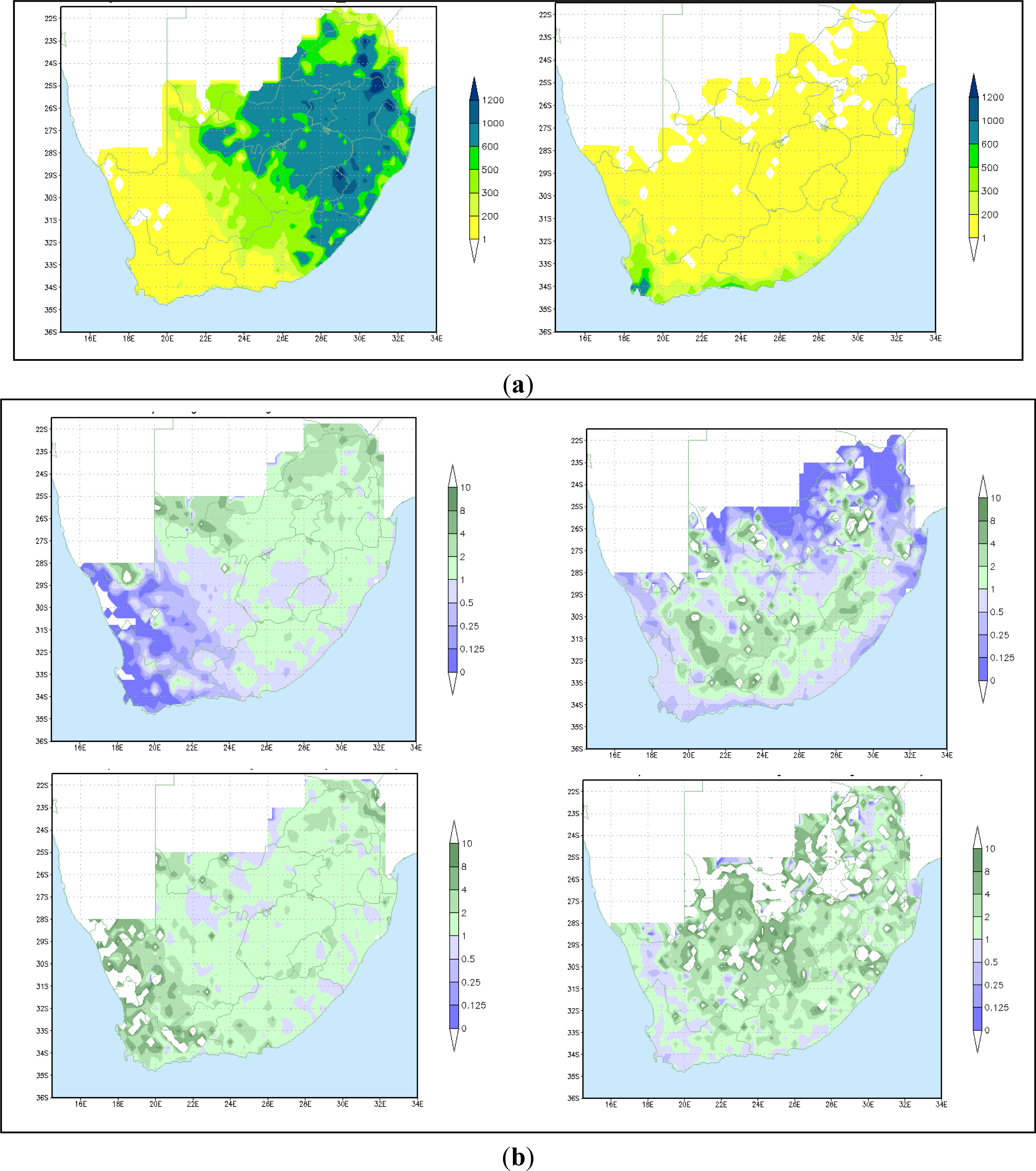
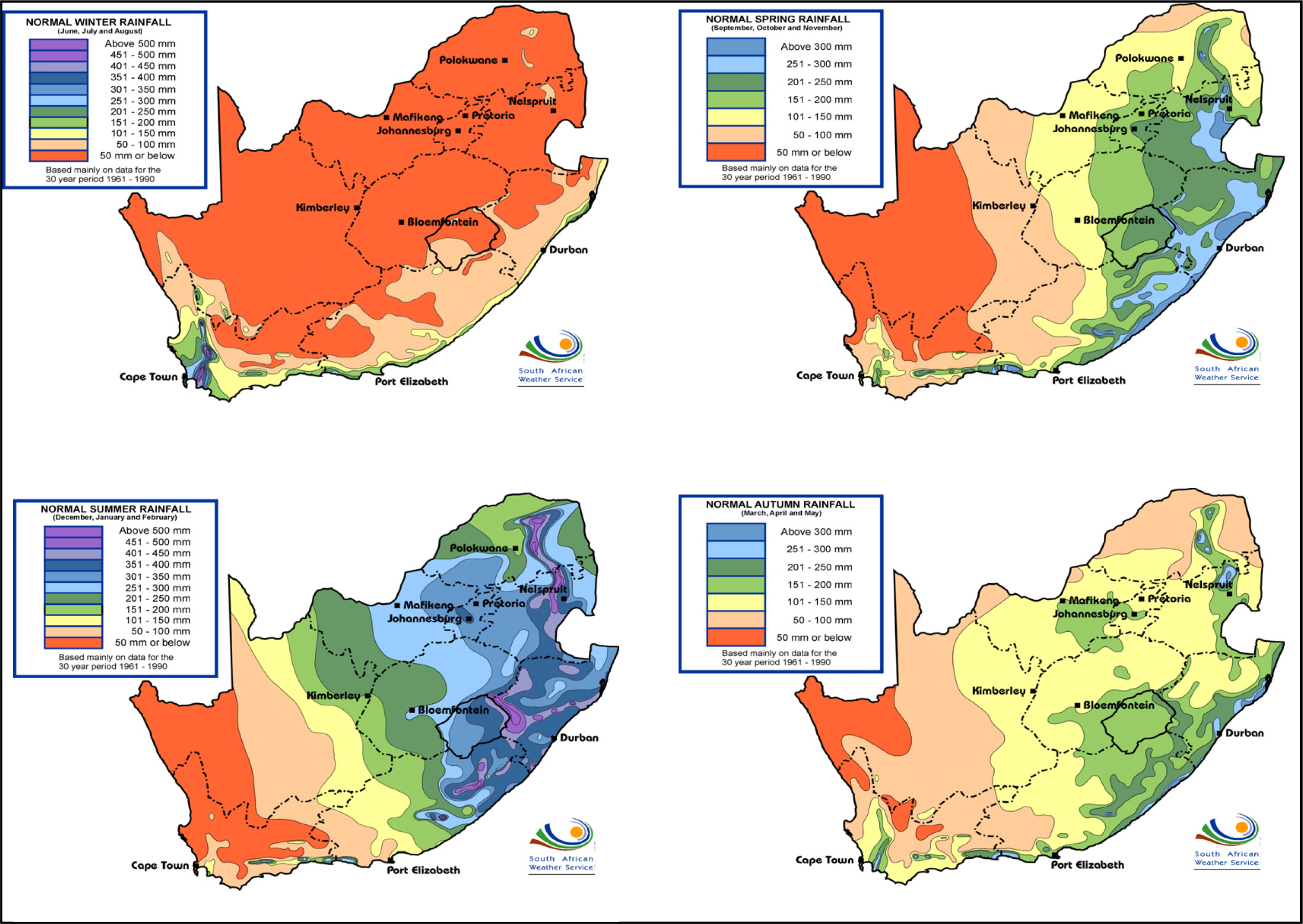
2.3. Seasonal Trends in Precipitation over South Africa

Rainfall patterns in South Africa, as prepared by Kruger [23] are depicted by Figure 1. This shows that the winter months (June, July and August) contribute very little to the annual rainfall amounts and that significant rainfall is restricted to the coastlines and adjacent interior of the country. Winter rainfall occurs mainly due to the passage of cold fronts and ridging high pressure systems in the form of stratiform rainfall. During spring (September to November) the rainfall gradually increases and the maximum contribution to the annual rainfall coincides with the summer months (December to February). In summer time the rainfall is mainly in the form of heat-driven convective thunderstorms. Rainfall gradually decreases in autumn (March to May). Convective as well as stratiform rainfall processes are thus important factors in the total rainfall in South Africa.

2.4. Precipitation Validation over South Africa

The International Precipitation Working Group [24] is one of the working groups of the Coordination Group for Meteorological Satellites (CGMS) [25], co-sponsored by CGMS and the World Meteorological Organization (WMO) [26]. The aim of this working group is to shed some light on operational and research satellite-based quantitative precipitation measurement opportunities and challenges. The IPWG not only compares different precipitation measurements from various satellite and model products around the world, but also provides standardized methods to verify these different methods against ground-truth datasets. The verification methodology is applied in various regions of the world by the participating members [2,27]. The precipitation estimates are compared with surface rain gauges or radar rainfall fields on a 0.25° × 0.25° grid, and are evaluated for 24 h periods. The South African Weather Service has been hosting a validating website for the South African region since March 2013. Various daily accumulations of model and satellite precipitation products are available on the South African IPWG validation webpage [28]. A threshold of 1 mm is used for evaluation purposes. The algorithms which are used for daily validation include: 3B42RT [29], CMORPH [30], CPCMMW [31,32], PERSIANN [33], GsMaP [34] and the Hydroestimator [35]. Table 1 lists the current satellite-based algorithms which are compared against 24 h accumulated rainfall as measured by the rain gauges at 06:00 UTC.
Several scores are used for the indication of skill in the IPWG suite of statistics including probability of detection (POD), probability of false detection (POFD), false alarm ratio (FAR), bias and Heidke Skills Score (HSS) as defined by [36]. Although all of these scores have some value, the HSS was chosen as a good overall indicator of skill since it gives an indication of the accuracy of the algorithm relative to that of chance. This score ranges from minus infinity to 1 with 0 indicating no skill and 1 being the perfect score [36]. The Heidke Skill Score is defined as:
HSS = ( Hits + Correct Negative ) ( expected correct ) random N ( expected correct ) random
where:
( expected correct ) random = 1 / N [ ( Hits + Misses ) ( Hits + False Alarms ) + ( Correct Negatives + Misses ) ( Correct Negatives + Flase ) Alams ) ]
During the period 18–21 April 2013 an upper-air disturbance caused heavy rainfall in excess of 50 mm per day in several places across the country. The maximum rainfall of more than 100 mm in 24 h was recorded at two locations in the south-eastern parts of the country on 20 April 2013. From 7 to 9 August 3012 another rainfall event was recorded, mainly affecting the south-western and southern coastlines of the country, due to the passage of a cold front. Rainfall figures of up to 50 mm were recorded on all three days, but most widespread heavy falls were recorded on 8 August 2013.
Figure 2 shows the HSS for each of these estimation techniques for the seven days evaluated during the two heavy rainfall events. All the statistics obtained were through comparisons with the rain gauge network. The Heidke Skill Score indicated that the best performing techniques were from the microwave sensors (especially 3B42RT, CMORPH and GSMaP). The local version of the HE compared well to the other products, although not out-performing them. The mean errors of the HE indicated significant overestimation in some cases but also underestimation in others. This result confirms the findings of [17] as well as the experience of using the HE over South Africa [21,22] namely: rainfall intensity can be overestimated during convective events, while warm rain processes can be missed or underestimated. In general terms, the HE is doing very well given the limitation of only using GEO input, but with the advantage of real-time availability.
Although these two events are not enough to conclusively determine any general results on the performance of the respective precipitation estimation techniques, these were the only significant rainfall events (which had an influence over a significant part of the country) that occurred since the IPWG methodology was introduced for the southern African region. Further statistical results will be gathered during the following seasons to substantiate these initial findings.

2.5. Goal of This Paper

In South Africa both convective and stratiform precipitation events play a role in different seasons and different areas of the country. Experience has shown that the Unified Model is most useful for synoptic-scale driven systems and the associated stratiform rainfall fields. The HE tends to be best for convective events and does not capture the stratiform events along the coast lines well. A first attempt to improve the satellite-based rainfall as input to the SAFFG was made in 2011 by de Coning and Poolman [21,22] by combining the HE with the stratiform rainfall field by the Unified Model (UMS). Using a combination of the HE and the UMS, a more comprehensive rainfall field was created.
The aim of this study is to describe an improved methodology to combine the HE with the UMS in order to enhance the input to the South African Flash Flood Guidance system, especially along the coastlines where wintertime stratiform rainfall events are often not captured by the HE. The new method will aim to address the short comings of the previous effort [21,22] and results will be shown to demonstrate the improvement in validation scores using sixty cases during the course of 2010.

3. Data and Methodology

3.1. Domain of Interest and Available Observation Data

The domain of interest is the area covering South Africa—south of 22°S and between 16°E and 33°E. The rain gauge network over the country includes 166 Automatic Weather Stations, 169 Automatic Rainfall Stations, 1,214 manual rainfall stations, and 199 synoptic stations. Figure 3 shows the location and density of these observations. Automatic gauges can provide hourly rainfall information, but unfortunately these observations are not enough for a comprehensive validation. In this study only the daily rainfall observations were used.
Rainfall fields from the Unified Model as well as the HE were limited to the area inside the boundaries of South Africa, using a mask to exclude the areas from neighbouring countries and/or oceans where no rain gauge data are available. Data from the UM and HE were initially at a resolution of 0.11° (or approximately 12 km).

3.2. Short-Comings and Improvements to Previous Methodology

In the initial attempt to improve the satellite-based rainfall as input to the SAFFG [21], it was shown that a combination of the HE and UMS (both bias corrected against the available rain gauges) evaluated better against rain gauge measurements than the HE on its own. This was specifically beneficial in cases when stratiform rainfall played a role along the coastlines of South Africa during the winter months.
Despite the improvements achieved by the combination of satellite and NWP rainfall fields, the method had its shortcomings:
(a)
The initial data set only focused on two years (2008 and 2009) for which the required data were available for the calculation of the biases.
(b)
An area average of the biases was calculated over the entire country, using a 0.5° × 0.5° grid box resolution.
(c)
For both rainfall fields, the area average bias corrections indicated that the HE and UMS always overestimate and thus the intensity of rainfall was always diminished in the combined product. However, applying an area average bias correction ignores the fact that the HE and the UMS fields overestimate in some regions and/or times of the year and underestimates in other regions and/or times of the year.
(d)
The data was divided into two 6-month seasons, November to April was treated as “summer” and May to October was treated as “winter” and the same bias correction was applied for the entire area for these two seasons.
As more data became available, new approaches were considered, which were applied in this study:
(a)
Five years of data (2008 to 2012) from the HE, the UMS and rain gauges were processed in order to establish whether a new, more realistic approach to an optimal satellite-based precipitation field, in combination with the NWP rainfall field, could be obtained.
(b)
The calculations were done on a monthly basis, instead of “seasonal”—in other words the monthly totals of rainfall from the different sources were compared to one another for the five year period. For the bias ratio of the HE, the total HE for each month was simply divided by the rainfall as measured by the rain gauges in that month for each grid box. A positive (negative) bias ratio indicated that the HE overestimated (underestimated) the rainfall. More detail on this methodology can be found in de Coning and Poolman (2011).
Similar to the methodology followed in [21], a proxy stratiform rain gauge rainfall quantity was calculated by using the ratio of the stratiform rainfall to the total rainfall field of the UM and applying the ratio to the rainfall amount from the rain gauges. The bias ratio of the UMS for each month was thus calculated by dividing the UMS by the proxy-stratiform quantity of the rain gauges in each grid box. A positive (negative) bias ratio indicates that the UMS overestimated (underestimated) the rainfall.
(c)
The resolution was improved to 0.25° × 0.25° grid boxes (similar to the IPWG validation methodology) for all calculations. This would imply that spatial variations in the bias patterns (over- and under-estimations) could be taken into account.

4. Results and Discussion

4.1. Bias Ratios for the Different Months

It was found that monthly bias ratios for HE and UMS ranged from 0.125 (underestimation) to 8 (overestimation) in more than 90% of the grid boxes over the South African domain in all months except July (>80%), August (>50%) and September (around 80%) (Figure 4). Values of more than 8 or less than 0.125 sometimes occurred on the edges of the domain or in grid boxes where very little data was available. During the winter months (July–September) much less rain is recorded and is mostly restricted to the coastlines. This can explain the smaller fraction of grid boxes within the 0.125 to 8 bias ratio range as a result of insufficient sampling.
The bias ratios for all 12 months cannot be shown here, but as an example, the gauge totals for January (summer) and July (winter) in the period considered are depicted in Figure 5a. The bias ratios of the HE and UMS for January and July, respectively, are shown in Figure 5b.
From Figure 5b it is clear that the HE underestimates the rainfall in the south-western parts of the country in January (top left), but overestimates the rainfall over the northeastern half of the country. In the summer months the dominant cause for rainfall is convection. In July (top right) overestimation occurs over the southern interior of the country and underestimation along the coastlines as well as in the far northeastern parts. It was previously shown [21] that overestimation often occurs in winter months when cold fronts approach the country in combination with a deep upper air trough, which causes widespread rainfall over the southwestern interior of the country. These cloud systems often reach high altitudes and consequently the very cold cloud top temperatures cause the HE to overestimate. Stratiform rainfall along the coastlines, which often accompanies the passage of shallow cold fronts and ridging surface high-pressure systems, is often missed or underestimated by the HE.
Also evident from Figure 5b is that the UMS generally overestimates slightly in January (bottom left) as well as in July (bottom right). However, in July underestimation also occurs along the southern coast lines.

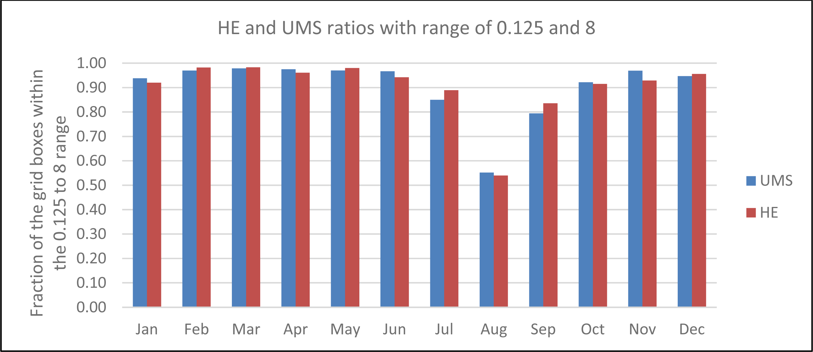
4.2. Combination of the HE and UMS Fields

Combining the two rainfall fields (HE and UMS) and their respective monthly bias corrections to create a more comprehensive rainfall pattern, was accomplished in the following manner:
  • If the bias ratio was in the range of 0.125 and 8, the bias correction was applied to the rainfall amount of the HE or UMS fields, respectively.
  • If the bias correction was less than 0.125 or more than 8, then four surrounding grid boxes were used to calculate an average of the bias ratio, if this average bias ratio was within the 0.125 to 8 range, the four-grid-boxes-average bias ratio was applied to the respective HE or UMS rainfall amounts.
  • If neither of the two previous calculations were within the 0.125 to 8 range, no bias correction was applied to the HE or UMS and the original rainfall value was kept unchanged.
The final combination field was simply the maximum value of the bias corrected HE or UMS fields. In this way, the combined precipitation field includes the convective rainfall events (best covered by the HE) as well as the stratiform rainfall events (best covered by the UMS) and extreme values are not missed, similar to the method followed by de Coning and Poolman [21].

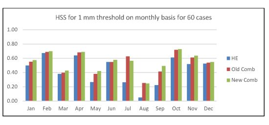
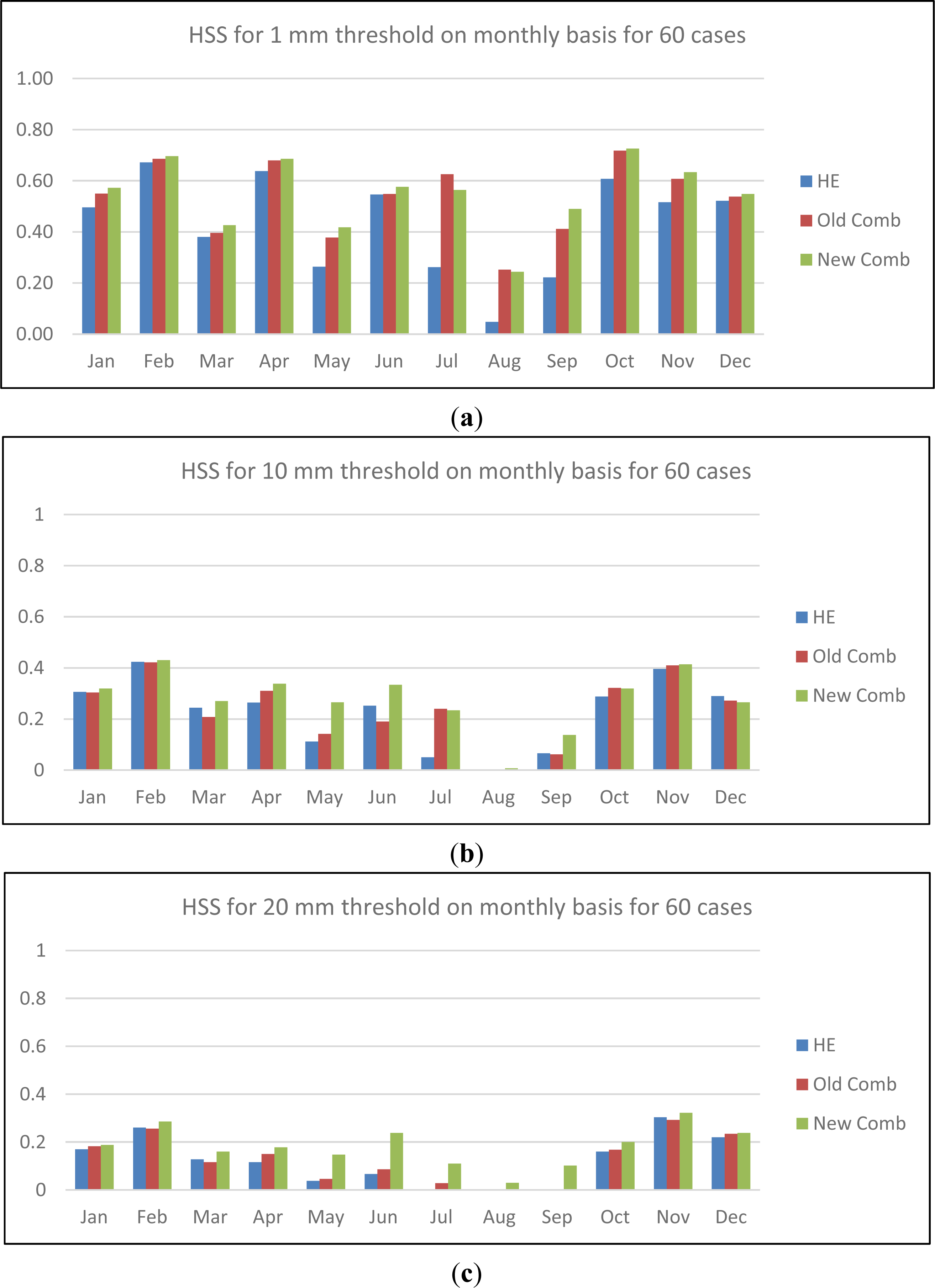
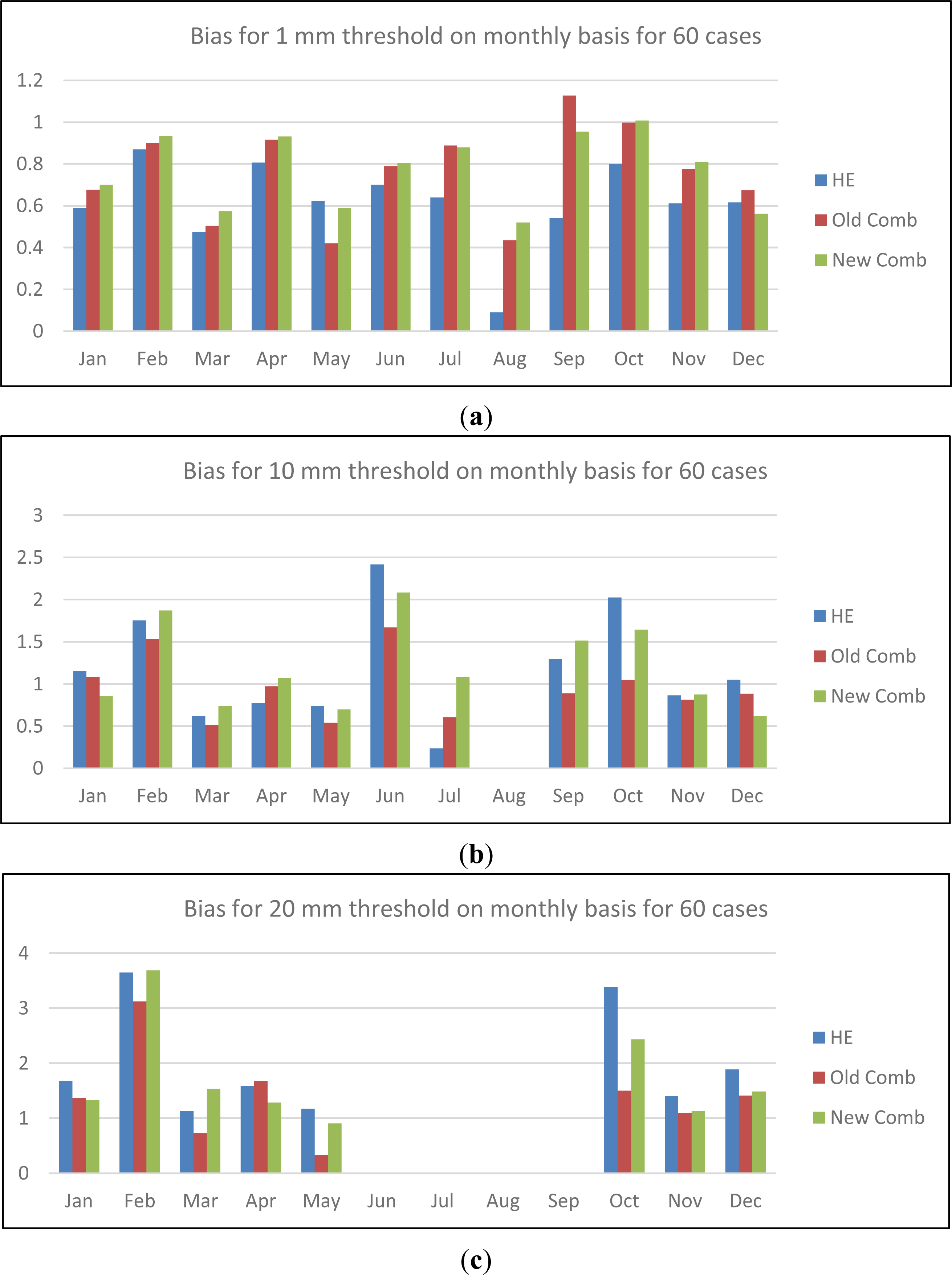
4.3. Comparing the Old Combination Methodology to the Proposed New Combination Methodology

In order to test whether the new methodology (using grid box-based, monthly bias ratios to combine the HE and UMS fields) would improve on (a) the HE without any corrections and (b) the previous methodology (using an area average bias ratio for two “seasons”), sixty cases were selected during 2010, five cases from each month of the year. Five days from each month were chosen when rainfall of different intensities was recorded over a significant area across the country. Cases from all the months were chosen to represent all the rain producing systems—convective as well as stratiform in nature. For each of these days, the HE, the new combination (New Comb) and the old combination (Old Comb) were statistically evaluated against the 24 h rain gauge totals. Daily totals were used for the validation purposes due to a lack of enough automatic rainfall reports to evaluate hourly rainfall. Daily thresholds of 1 mm, 10 mm and 20 mm were chosen to also evaluate the skill of the methods to estimate rainfall intensity.

4.3.1. Results for Each Month, Using Five Cases per Month

In Figure 6a–c the HSS of the five cases per month was used to calculate an average for each month and for the three different thresholds. Figure 6a shows the skill of the different methods using 1 mm threshold. Using the HE without any bias correction (blue bars) has the smallest HSS in all the months, the Old Comb (red bars) show some improvement, while the New Comb (green bars) performed the best in all the months. The only exceptions are July and August, where New Comb is slightly worse than Old Comb. From Figure 6b it is clear that New Comb also outperforms the HE and Old Comb for the 10 mm threshold in most months. In Figure 6c the indication is that the HSS of New Comb is better than the others for the 20 mm threshold in all the months.
A significant improvement is noted in the months of May to September, which are the months when the frontal passages along the coastlines of the country are accompanied by stratiform rainfall. These are the cases that the HE alone could have missed and that Old Comb (using seasonal, area averaged bias ratios) could have underestimated. The New Comb (using grid box-based bias ratios) shows that both the HE and UMS are underestimating in these regions and should be corrected upwards. The effect of this approach is that rainfall along the coastal areas is augmented.
In Figure 7a–c the Bias scores (or frequency bias) defined by Wilks [37] are shown for the different thresholds (1–20 mm). A perfect score is one, while values more (less) than 1 indicate overestimation (underestimation). This score establishes how well the estimate frequency of “yes” events compares to the observed frequency of “yes” events. For the 1 mm threshold (Figure 7a), it can be seen that New Comb improves the Bias score (gets it closer to 1) in almost all the months. A similar result is found for the 10 mm threshold (Figure 7b). In August very few grid boxes with rainfall of more than 10 mm were available for the score calculation and thus the bias score was omitted. Similarly, very little rainfall grid boxes with rain more than 20 mm were available for calculation of the bias score (Figure 6c) in June to August and thus the bias scores were omitted. In general the New Comb improves the bias score, i.e., lowers it if it is more than 1 and augments it when it is less than 1 in most months.
Figure 8 summarizes the HSS for all the cases and it is clear that the New Comb outperforms the other methods. Table 2 summarizes the percentages cases for which the HSS of the New Comb was better than or the same as the Old Comb and the uncorrected HE for the different thresholds.

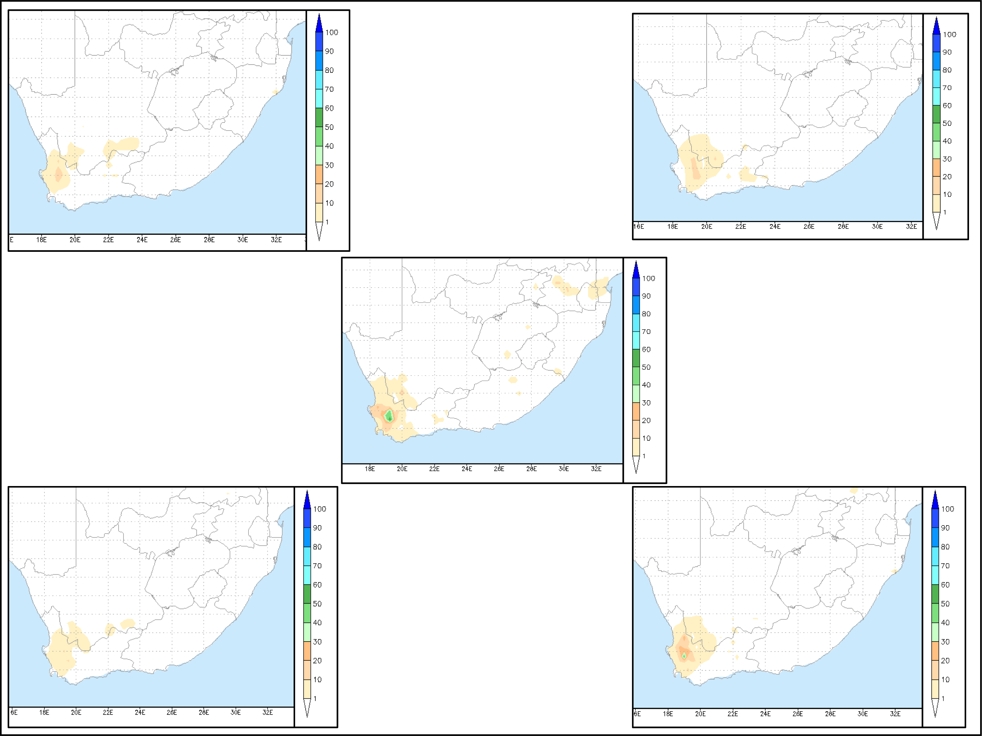
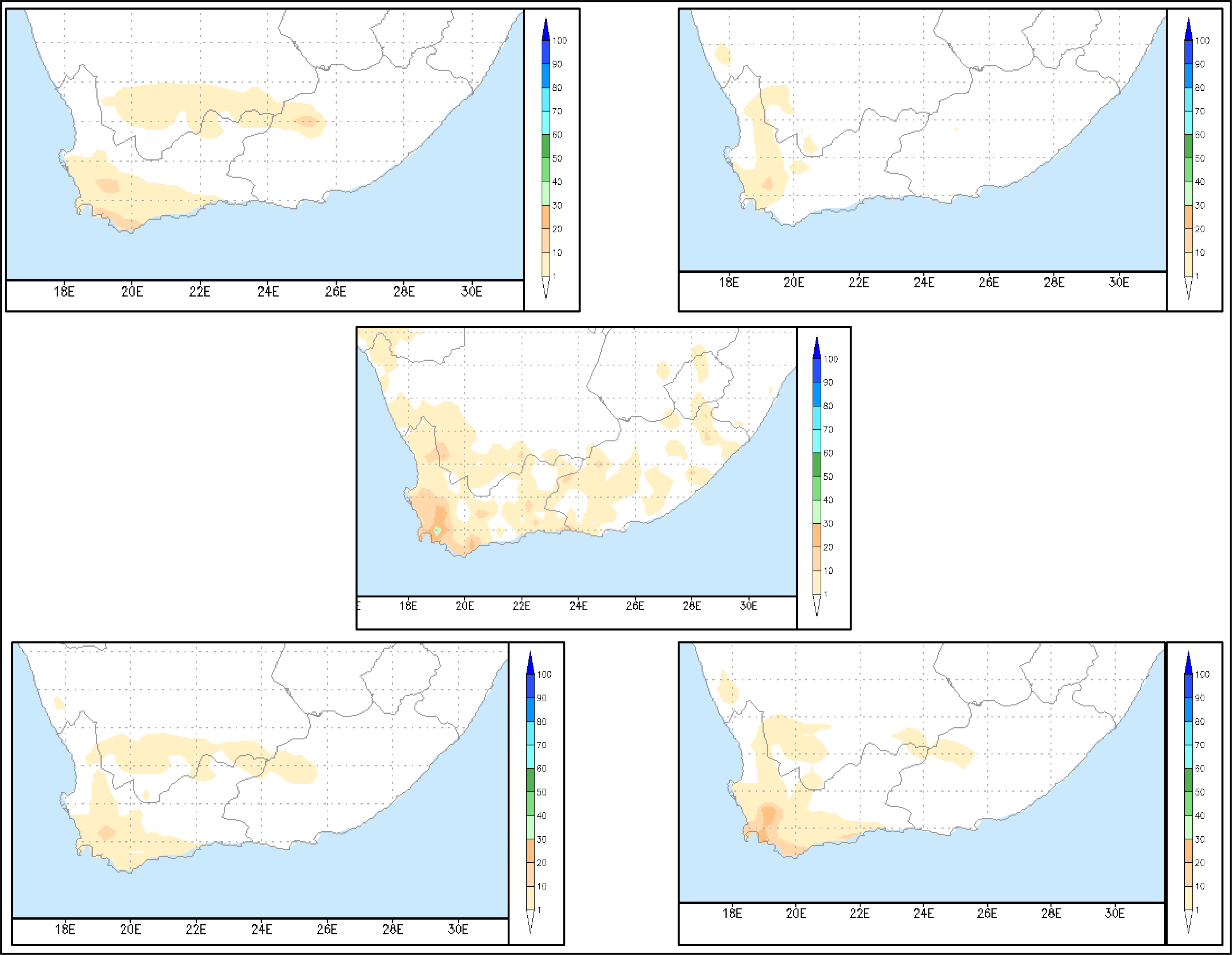
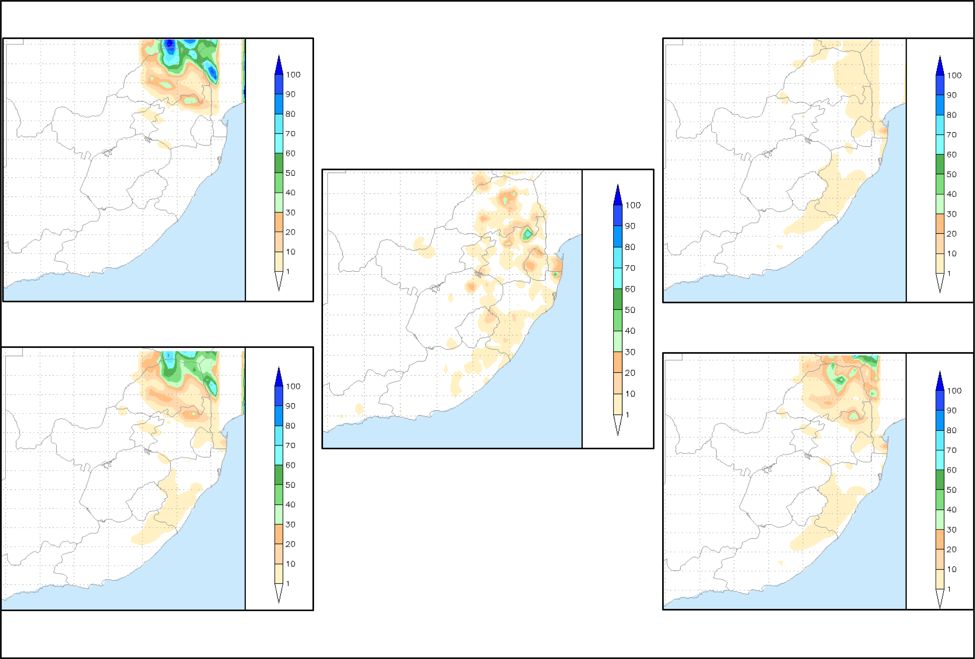
4.3.2. Results for Individual Days

In order to observe the influence of the bias ratio adjustments in more detail over different areas of the country on a daily basis, a few cases in different months are presented.

Case 1: 28 January 2010

On 28 January 2010 widespread summer rain fell over the eastern half of the country (Figure 9 middle), with most of the rain in the northeastern part (>30 mm). The HE (Figure 9 top left) estimated heavier falls too far north and did not capture the rain which fell over the south-eastern interior. The UMS (Figure 9 top right) underestimated the heavier falls in the northeast but included the lighter falls in the southeast. The Old Comb (Figure 9 bottom left) made the HE less intense in the north and added the stratiform rainfall from the UMS in the southeastern parts. The rainfall in the north was, however, still too much, compared to the rain gauge totals. The New Comb (Figure 9 bottom right) brought the intensity of the rain down even more than the Old Comb (and thus closer to the observation) and also reflected the stratiform rainfall in the southeastern parts. The HSS for the 1 mm threshold increased from 0.61 (Old Comb) to 0.64 (New Comb). For the 10 mm threshold there was an increase from 0.32 (Old Comb) to 0.36 (New Comb) and for 20 mm a 6% increase to 0.30 (New Comb).

Case 2: 10 May 2010

On this autumn day most of the rainfall was recorded (Figure 10 middle) over the southwestern part of the country, with some falls in excess of 30 mm in the southwest. The HE (Figure 10 top left) did capture some of this rainfall, but underestimated it. The UMS field (Figure 10 top right) also underestimated the rainfall in this area. The Old Comb (Figure 10 bottom left) decreased the amount of rainfall from both fields and thus indicated even less rain in the area. The New Comb could enhance the rainfall from HE and UMS based on the grid box-based bias ratios and thus captured the heavier falls very well. The HSS for the 1 mm threshold increased from 0.49 (Old Comb) to 0.57 (New Comb). For the 10 mm threshold the HSS increased from 0.11 (Old Comb) to 0.49 (New Comb). For 20 mm the Old Comb did not estimate any rainfall above 20 mm and thus the HSS was 0, while the New Comb could get a HSS of 0.37. The New Comb clearly made a huge improvement in capturing a more realistic rainfall picture.

Case 3: 12 June 2010

On this winter day most of the rainfall was recorded (Figure 11 middle) over the southwestern part of the country. The HE (Figure 11 top left) did very well in capturing the rainfall, although overestimating it slightly. The UMS field (Figure 11 top right) underestimated the rainfall. The Old Comb (Figure 11 bottom left) decreased the amount of rainfall from both fields. The New Comb successfully enhanced the rainfall from HE and UMS using the grid box-based bias ratios and this captured the area where the higher falls (20–30 mm) occurred, but overestimated the values slightly. The HSS for the 1 mm threshold increased from 0.66 (Old Comb) to 0.69 (New Comb). For the 10 mm threshold the Old Comb did not estimate any rainfall exceeding this threshold and thus the HSS was zero, while the New Comb could get a HSS of 0.28. No rainfall of more than 20 mm was recorded by the rain gauges. The New Comb improved the precipitation intensity giving a more representative rainfall picture, although slightly overestimating the peak rainfall.

Case 4: 13 June 2010

In this winter time case, stratiform precipitation covered the southwestern and southern parts of the country. Heavier falls (>30 mm) were recorded in the southwest (Figure 12 middle). The HE (Figure 12 top left) captured some of the rainfall, but both area and intensity was underestimated. The UMS field (Figure 12 top right) underestimated the rainfall. The Old Comb (Figure 12 bottom left) decreased the amount of rainfall from both fields. The New Comb could adjust the rainfall from HE and UMS fields based on the grid box-based bias ratios and this did well to capture the area where the higher falls occurred, but slightly underestimated the peak. The lighter falls on the southern parts of the country could not be included since it was not captured by the HE or the UMS. The HSS for the 1 mm threshold increased with 4 percentage points to 0.40 (New Comb). For the 10 mm threshold the HSS increased from 0.02 (Old Comb) to 0.30 (New Comb) and for the 20 mm threshold the HSS of the Old Comb was zero, but this improved to 0.44 (New Comb).

Case 5: 29 November 2010

Summer convection occurred over the eastern parts of the country (Figure 13 middle), with the heaviest falls recorded in the north with rainfall in excess of 40mm. The HE (Figure 13 top left) did well in capturing the rainfall, but overestimated it slightly on the eastern border of the country. The UMS field (Figure 13 top right) underestimated the rainfall. The Old Comb (Figure 13 bottom left) decreased the amount of rainfall from both fields and added the rainfall along the southeastern coastline. The New Comb could adjust the rainfall from HE and UMS fields using the new methodology and this captured the area where the higher falls occurred quite well, but slightly underestimated the peak in the far north. The HSS for the 1 mm threshold remained the same (0.68) and slightly decreased from 0.4 (Old Comb) to 0.38 (New Comb) for the 10 mm threshold. For the 20 mm threshold the HSS increased from 0.08 (Old Comb) to 0.24 (New Comb).

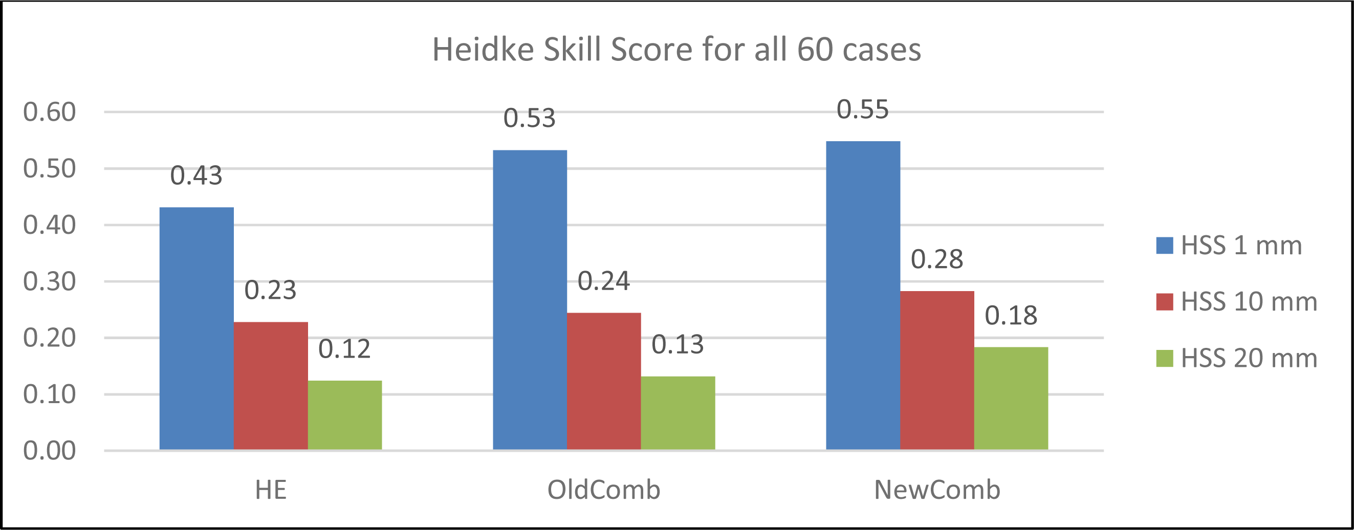
4.3.3. Summary of Results

A new way of combining the HE and UMS fields was proposed, based on the results obtained with five years of data from 2008 to 2012 to calculate a 0.25° × 0.25° grid box-based bias ratio for the HE and UMS precipitation fields, on a monthly basis. The new methodology takes into account that the HE and UMS fields can overestimate as well as underestimate the rainfall intensity and that this bias correction can change temporally (for different months) as well as spatially.
Sixty cases from 2010, five cases in each month of the year, were used to compare the uncorrected HE, the old combination (Old Comb) and the new combination (New Comb) of the HE and UMS fields to the rainfall observed by the rain gauges. The monthly averages of the HSS indicate that the New Comb is more accurate than the Old Comb as well as better than the uncorrected HE for the 1 mm, 10 mm as well as the 20 mm thresholds in most months. The monthly averages of the Bias Score show that the New Comb is improving the Bias Score for the majority of the months. The biggest improvement is in the winter months when stratiform rainfall events influence the coastal areas of the country.
Five daily cases were considered in more detail and in these the advantage of using monthly, grid box-based bias ratios is evident since the contributions of the UMS and HE were allowed to vary spatially. It is shown that the New Comb can provide a more accurate and representative rainfall field than the uncorrected HE and the Old Comb on a daily basis.
Remotely sensed rainfall estimation is a valuable tool for forecasters in order to nowcast precipitation. The combination of rainfall fields from HE and UMS presented here can be calculated on an hourly basis and will provide a comprehensive rainfall field needed for the nowcasting of precipitation. The South African Flash flood Guidance requires input of rainfall observations on time scales of less than 6 h in order to provide a nowcast of such events. Rainfall fields from rain gauges, radar rainfall as well as satellite rainfall are used as input to the SAFFG on an hourly, 3-hourly and 6-hourly basis. It would have been ideal to validate the new combination product on this shorter time scale, but unfortunately not enough observation data are available for such a validation. Given the improvement shown on a daily basis, it is believed that the combination of HE and UMS rainfall field should benefit the nowcasting of precipitation as well as enhance input to the South African Flash Flood Guidance system if it is used on an hourly, 3-hourly and 6-hourly basis as a supplement to input from radar rainfall and rain gauge data.

5. Conclusions

The goal of this paper was to improve on a previously defined method to combine the Hydroestimator and the stratiform rainfall field from the Unified Model to create a precipitation field which can capture both convective as well as stratiform rainfall events. The latter is specifically important in South Africa since stratiform rainfall impacts on the coastal areas of the country during winter months, when shallow cold fronts or ridging surface high-pressure systems induce winter rainfall. The shortcomings of the old methodology (Old Comb) was highlighted and addressed to create a new, grid box-based bias corrected and combined rainfall field. The monthly averages of the 60 cases of the HSS and Bias Score for the new method (New Comb) improved for most of the months when compared to the uncorrected HE as well as the Old Comb. For the 1mm, 10mm and 20mm thresholds the HSS of the new methodology (New Comb) was 12%, 5% and 6%, respectively, better than using the uncorrected HE. The New Comb was better than the Old Comb in 67% of the cases for the 1mm threshold, 54% of the cases for the 10mm threshold and 48% of the cases for the 20mm threshold. Significant improvement for the New Comb was shown in the winter months, especially for cases when more than 20mm of rain was recorded. The five daily cases shown here, indicate that the New Comb can address spatial differences over the interior and coastlines of the country to yield better results than the other techniques. It was shown that using a grid box-based bias correction for both the HE and UMS fields, based on monthly data for five years, can provide more accurate estimates of the HE and UMS fields to contribute to the combined precipitation product. In this way, both stratiform and convective rainfall events can be captured using input from GEO satellite as well as numerical weather prediction models to create a near-real time comprehensive rainfall estimate.
As more years of data become available, it is foreseen that the climatology with which the bias ratios were calculated could be extended. The Nowcasting Satellite Application Facility has developed various applications of the Meteosat data. One of these is a Convective Rainfall Rate (CRR) [38]. This methodology uses three of the MSG channels, together with input from NWP to create a near-real-time rainfall product. Although this product also focuses on convective rainfall, it is a candidate for future investigation. The Nowcasting SAF software is being implemented in South Africa and the latest version of the CRR product will be tested as a GEO precipitation estimator over the South African domain in the near future. A robust evaluation framework and benchmark have now been established to test whether this product will outperform existing methods.

Acknowledgments

I would like to acknowledge the assistance of Bathobile Maseko for the processing of data for this study as well as Cassandra Pringle for the work on the IPWG case studies. This work was done as part of the project funded by the Water Research Commission (WRC) in South Africa.

Conflicts of Interest

The author declares no conflict of interest.

References and Notes

  1. Huffman, G.J.; Adler, R.F.; Arkin, P.; Chang, A.; Ferraro, R.; Gruber, A.; Janowiak, J.; McNab, A.; Rudolf, B.; Schneider, U. The Global Precipitation Climatology Project (GPCP) combined precipitation dataset. Bull. Amer. Meteorol. Soc 1997, 78. [Google Scholar]
  2. Kidd, C.; Bauer, P.; Turk, J.; Huffman, G.J.; Joyce, R.; Hsu, K.-L.; Braithwaite, D. Intercomparison of high-resolution precipitation products over northwest Europe. J. Hydrometeorol 2012, 13, 67–83. [Google Scholar]
  3. NOAA STAR—Centre for Satellite Applications and Research. Available online: http://www.star.nesdis.noaa.gov/smcd/emb/ff/index.php (accessed on 22 July 2013).
  4. De Coning, E. Satellite Applications for Very Short Range Weather Forecasting Systems in Southern African Developing Countries. In Recent Advances in Satellite Research and Development, 1st ed; Gardiner, S., Olsen, K.P., Eds.; Nova Science Publishers, Inc: Hauppauge, NY, USA, 2013; pp. 67–92. [Google Scholar]
  5. IPWG Data sets. Available online: http://www.isac.cnr.it/~ipwg/data/datasets.html (accessed on 22 July 2013).
  6. EUMETSAT Current Satellites. Available online: http://www.eumetsat.int/website/home/Satellites/CurrentSatellites/Meteosat/index.html (accessed on 22 July 2013).
  7. EUMETSAT Satellite Application Facilities. Available online: http://www.eumetsat.int/website/home/Satellites/GroundSegment/Safs/index.html/ (accessed on 22 July 2013).
  8. Schmetz, J.; Pili, P.; Tjemkes, S.; Just, D.; Kerkmann, J; Rota, S.; Ratier, A. An introduction to Meteosat Second Generation (MSG). Bull. Amer. Meteorol. Soc 2002, 83, 977–992. [Google Scholar]
  9. EUMETSAT Data Products. Available online: http://www.eumetsat.int/website/home/Data/Products/index.html (accessed on 22 July 2013).
  10. Kothe, S.; Good, E.; Obregon, A.; Ahrens, B.; Nitsche, H. Satellite-based sunshine duration for Europe. Remote Sens 2013, 5, 2943–2972. [Google Scholar]
  11. Olsen, J.; Ceccato, P.; Proud, S.; Fensholt, R.; Grippa, M.; Mougin, E.; Ardo, J.; Sandholt, I. Relation between seasonally detrended shortwave infrared reflectance data and land surface moisture in semi-arid Sahel. Remote Sens 2013, 5, 2898–2927. [Google Scholar]
  12. Romano, F.; Ricciardelli, E.; Cimini, D.; Di Paola, F.; Viggiano, M. Dust detection and optical depth retrieval using MSG-SEVIRI data. Atmosphere 2013, 4, 35–47. [Google Scholar]
  13. Marchese, F.; Ciampa, M.; Filizzola, C.; Lacava, T.; Mazzeo, G.; Pergola, N.; Tramutoli, V. On the exportability of Robust Satellite Techniques (RST) for active volcano monitoring. Remote Sens 2010, 2, 1575–1588. [Google Scholar]
  14. Vincente, G.; Scofield, R.A.; Mentzel, W.P. The operational GOES infrared rainfall estimation technique. Bull. Amer. Meteorol. Soc 1988, 79, 1883–1898. [Google Scholar]
  15. Davies, T.; Cullen, M.J.P.; Malcolm, A.J.; Mawsom, M.H.; Staniforth, A.; White, A.A.; Wood, N. A new dynamical core for the Met Office’s global and regional modelling of the atmosphere. Quart. J. R. Meteorol. Soc 2005, 131, 1759–1782. [Google Scholar]
  16. IPWG Singles Source Data Set. Available online: http://www.isac.cnr.it/~ipwg/data/datasets3.html (accessed on 22 July 2013).
  17. Kuligowski, R.J.; Qiu, S.; Scofield, R.A.; Gruber, A. The NESDIS QPE Verification Program. Proceedings of the 11th Conference on Satellite Meteorology and Oceanography, Madison, WI, USA; 2001. [Google Scholar]
  18. Poolman, E.R.; Chikoore, H.; Lucio, F. Public benefits of the severe weather forecasting demonstration project in South-Eastern Africa. WMO Newsl. MeteoWorld. December 2008. Available online: http://www.wmo.int/pages/publications/meteoworld/archive/dec08/index_en.html (accessed on 18 July 2013).
  19. Georgakakos, K.P. Analytical results for operational flash flood guidance. J. Hydrol 2006, 317, 81–103. [Google Scholar]
  20. Georgakakos, K.P. Mitigating Adverse Hydrological Impacts of Storm on a Global Scale with High Resolution: Global Flash Flood Guidance. Proceedings of the International Conference on Storms, Storms Science to Disaster Mitigation, Brisbane, QLD, Australia, 2004.
  21. De Coning, E.; Poolman, E.R. South African weather service operational satellite-based precipitation estimation technique: Applications and improvements. Hydrol. Earth Syst. Sci 2011, 15, 1131–1145. [Google Scholar]
  22. De Coning, E. Satellite-based precipitation estimation techniques for operational use over southern Africa. Proceeding of the 16th SANCIAHS National Hydrology Symposium, Pretoria, South Africa, 1–4 October 2012; Available online: http://www.ru.ac.za/static/institutes/iwr/SANCIAHS/2012/ (accessed on 1 August 2013).
  23. Kruger, A.C. Climate of South Africa, Precipitation; Report No. WS47; South African Weather Service: Pretoria, South Africa, 2007; pp. 1–41. [Google Scholar]
  24. IPWG. Available online: http://www.isac.cnr.it/~ipwg// (accessed on 22 July 2013).
  25. CGMS. Available online: http://www.cgms-info.org/ (accessed on 22 July 2013).
  26. WMO. Available online: http://www.wmo.int/pages/index_en.html (accessed on 22 July 2013).
  27. Ferraro, R.; Kidd, C.; Arkin, P.; Turk, J. Satellite Precipitation Activities of the International Precipitation Working Group. Proceedings of the 23rd AMS Conference on Hydrology, Phoenix, AZ, USA, 2013. Abstract 5B.1..
  28. IPWG Validation. Available online: http://www.isac.cnr.it/~ipwg/validation.html (accessed on 22 July 2013).
  29. Huffman, G.J. The TRMM Multisatellite Precipitation Analysis (TMPA): Quasi-global, multiyear, combined-sensor precipitation estimates at fine scales. J. Hydrometeorol 2007, 8, 38–55. [Google Scholar]
  30. Joyce, R.J.; Janowiak, J.E.; Arkin, P.A.; Xie, P. CMORPH: A method that produces global precipitation estimates from passive microwave and infrared data at high spatial and temporal resolution. J. Hydrometeorol 2004, 5, 487–503. [Google Scholar]
  31. Purdom, J.F.W.; Dills, P.N. Cloud Motion and Height Measurements from Multiple Satellites Including Cloud Heights and Motions in Polar Regions. Proceedings of the Seventh Conference on Satellite Meteorology and Oceanography, Monterey, CA, USA, 1994.
  32. Janowiak, J.E.; Joyce, R.J.; Yarosh, Y. A real-time global half-hourly grid box-resolution infrared dataset and its applications. Bull. Amer. Meteorol. Soc 2001, 82, 205–217. [Google Scholar]
  33. Sorooshian, S.; Hsu, K.-L.; Gao, X.; Gupta, H.V.; Iman, B.; Braithwaite, D. Evaluation of PERSIANN system satellite-based estimates of tropical rainfall. Bull. Amer. Meteorol. Soc 2000, 81, 2035–2046. [Google Scholar]
  34. Kubota, T.; Shige, S.; Hashizume, H.; Aonashi, K.; Takahashi, N.; Seto, S.; Takayabu, Y.N.; Ushio, T.; Nakagawa, K.; Iwanami, K.; et al. Global precipitation map using satellite-borne microwave radiometers by the GSMaP project: Production and validation. IEEE Trans. Geosci. Remote Sens 2007, 45, 2259–2275. [Google Scholar]
  35. Scofield, R.A.; Kuligowski, R.J. Status and outlook of operational satellite precipitation algorithms for extreme events. Wea. Forecast 2003, 18, 1037–1051. [Google Scholar]
  36. Wilks, D.S. Statistical Methods in Atmospheric Sciences, 2nd ed.; Elsevier Science & Technology Books: Amsterdam, The Netherlands, 2006. [Google Scholar]
  37. Forecast verification issues, methods and FAQ. Available online: http://www.cawcr.gov.au/projects/verification/#Standard_verification_methods (accessed on 19 July 2013).
  38. Nowcasting Satellite Application Facility. Available online: https://www.nwcsaf.org/HD/Main.jsp(accessed on 23 July 2013).
Figure 1. Seasonal distribution of rainfall over a 30 year period: Winter rainfall (top left), spring rainfall (top right), summer rainfall (bottom left) and autumn rainfall (bottom right), after [23].
Remotesensing 05 05702f1
Figure 2. Heidke Skill Scores for seven cases in 2013 for all the estimation techniques.
Remotesensing 05 05702f2
Figure 3. Density and location of Automatic Weather Stations (left) and manual and synoptic rainfall stations (right).
Remotesensing 05 05702f3
Figure 4. Fraction of the amount of grid boxes covered across the country where the month bias ratios for HE (red) and UMS (blue) ranged between 0.125 and 8.
Remotesensing 05 05702f4
Figure 5. (a) Rain gauge totals for January (left) and July (right) for the five year period from 2008 to 2012. (b) Bias ratios for HE in January (top left) and July (top right). Bias ratios for UMS in January (bottom left) and July (bottom right). Purple colours indicate underestimation and green colours indicate overestimation.
Remotesensing 05 05702f5
Figure 6. Heidke Skill Scores for (a) 1 mm threshold, (b) 10 mm threshold and (c) 20 mm threshold for all 60 cases (5 cases per month). HSS of the HE is in blue, for Old Comb in red and for New Comb in green.
Remotesensing 05 05702f6
Figure 7. Bias score for (a) 1 mm threshold, (b) 10 mm threshold and (c) 20 mm threshold for all 60 cases (5 cases per month). Bias score of the HE is in blue, for Old Comb in red and for New Comb in green.
Remotesensing 05 05702f7
Figure 8. HSS for all 60 cases for 1 mm, 10 mm and 20 mm thresholds.
Remotesensing 05 05702f8
Figure 9. Case 1: 28 January 2010. HE (top left), UMS (top right), Old Comb (bottom left), New Comb (bottom right) and rainfall measured by gauges (middle).
Remotesensing 05 05702f9
Figure 10. Case 2: 10 May 2010. HE (top left), UMS (top right), Old Comb (bottom left), New Comb (bottom right) and rainfall measured by gauges (middle).
Remotesensing 05 05702f10
Figure 11. Case 3: 12 June 2010. HE (top left), UMS (top right), Old Comb (bottom left), New Comb (bottom right) and rainfall measured by gauges (middle).
Remotesensing 05 05702f11
Figure 12. Case 4: 13 June 2010. HE (top left), UMS (top right), Old Comb (bottom left), New Comb (bottom right) and rainfall measured by gauges (middle).
Remotesensing 05 05702f12
Figure 13. Case 4: 29 November 2010. HE (top left), UMS (top right), Old Comb (bottom left), New Comb (bottom right) and rainfall measured by gauges (middle).
Remotesensing 05 05702f13
Table 1. Different satellite-based algorithms which are validated over the South African domain.
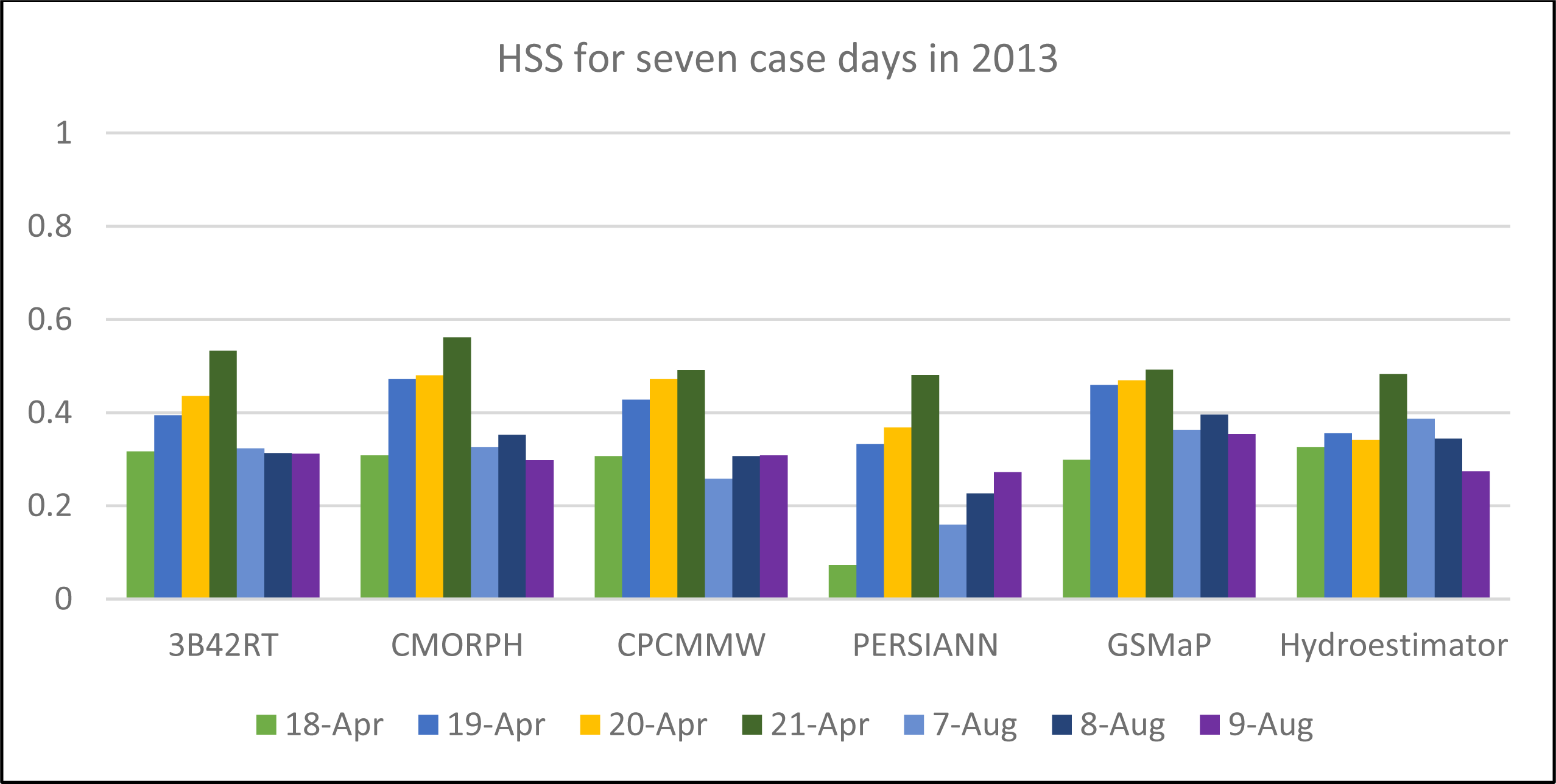
Satellite algorithms combining microwave sensors and GEO input:

3B42RTTRMM merged passive microwave data and microwave-calibrated IR data
CMORPHMultiple microwave polar-orbiter satellites with spatial propagation using GEO IR data
CPCMMWMultiple microwave polar-orbiter satellites with no IR data propagation or morphing
PERSIANNPrecipitation intensity and distribution initially trained using ground radar and microwave satellite observations for data assimilation. GEO IR data merged with assimilated data
GSMaPUses GEO Infrared data combined with Microwave Polar orbiter data

Satellite algorithm using only GEO input:

HydroestimatorUses GEO IR data combined with NWP fields.
Table 2. Summary of the percentages cases for which the HSS of the New Comb is the same as or exceeds the HSS of the other two methods.
New Comb Has a Better HSS than Old CombNew Comb Has a HSS the Same as Old CombNew Comb Has a Better HSS than Uncorrected HE
1 mm threshold67%13%93%
10 mm threshold54%25%51%
20 mm threshold48%41%53%

