Quantitative Analysis of the Waterline Method for Topographical Mapping of Tidal Flats: A Case Study in the Dongsha Sandbank, China


Abstract
:1. Introduction
2. Study Area and Datasets
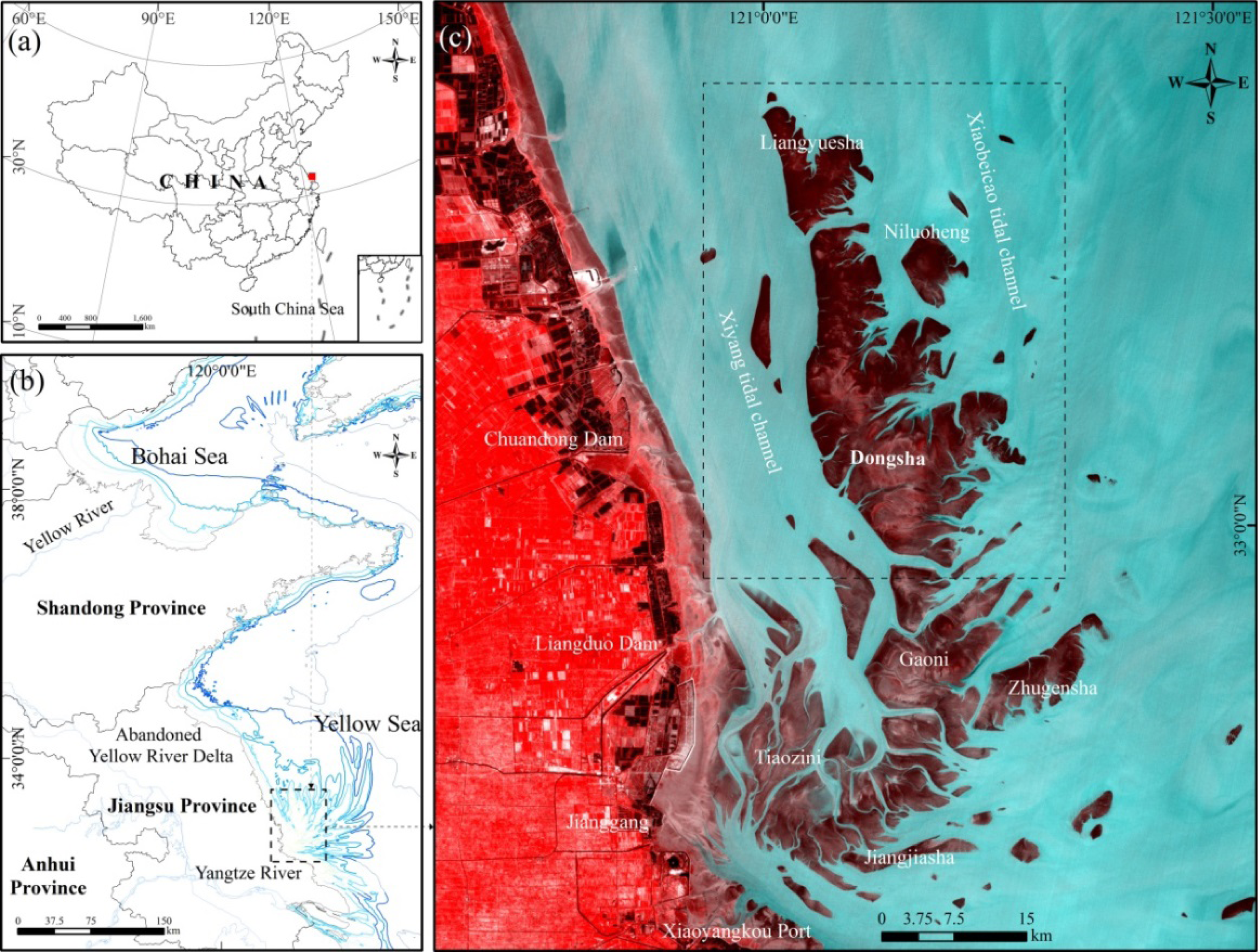
2.1. Study Area
2.2. Datasets
- (1)
- Preview satellite images. A total of 2,494 preview satellite images that cover the study area were collected. The images were taken from common civilian medium resolution satellite sensors, including the Landsat Multispectral Scanner System (MSS) [27], Thematic Mapper (TM) [28], Enhanced Thematic Mapper Plus (ETM+) [28], Japanese Marine Observation Satellite (MOS) [29], Multispectral Electronic Self-Scanning Radiometer (MESSR) [29], Japanese Earth Resources Satellite (JERS) [29], Synthetic Aperture Radar (SAR) [28], Indian Remote-Sensing Satellite (IRS) Linear Imaging Self-Scanning Sensor (LISS) and Advanced Wide-Field Sensor (AWiFS) [28], China-Brazil Earth Resources Satellite (CBERS) Charge Coupled Device (CCD) [30], Chinese Beijing-1 CCD and HJ CCD [31], European Remote-Sensing Satellite (ERS) SAR and the Environmental Satellite (Envisat) Advanced Synthetic Aperture Radar (ASAR) [28]. Details of the image sources are listed in Table 1. Of all the preview images, 852 images are high-quality (cloud-free and containing clear waterlines).
- (2)
- Medium spatial-resolution satellite images. A total of 231 medium-resolution satellite images taken during different tidal periods in 1973–1977, 1980–1981, 1990–1991, 2000, 2006, 2007, 2008, 2009,and 2010 were obtained from several sensors, including Landsat MSS/TM/ETM+, MOS-1 MESSR, SPOT HRV, IRS-P6 LISS/AWiFS, CBERS-1/2 CCD, Beijing-1 CCD, HJ-1 A/B CCD, JERS SAR and ERS-1/2 SAR (Table 2). The spatial resolution of these satellite images varies from 10 m to 80 m. All the satellite images are of high-quality.
- (3)
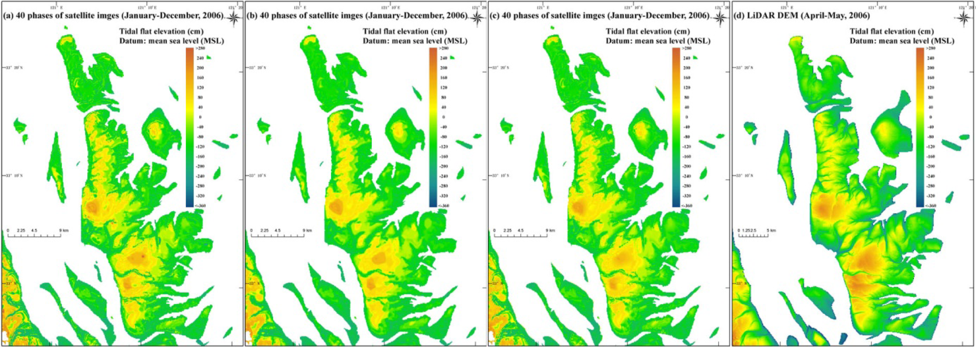
- Airborne elevation data. LiDAR data were collected in April and May 2006, by the Jiangsu Provincial Bureau of Surveying, Mapping and Geo-information. The LiDAR DEMs provided to the research team had a vertical accuracy of less than 15 cm and were resampled to a 5 m × 5 m grid.
3. The Rationale of the Waterline Method and Its Potential Errors
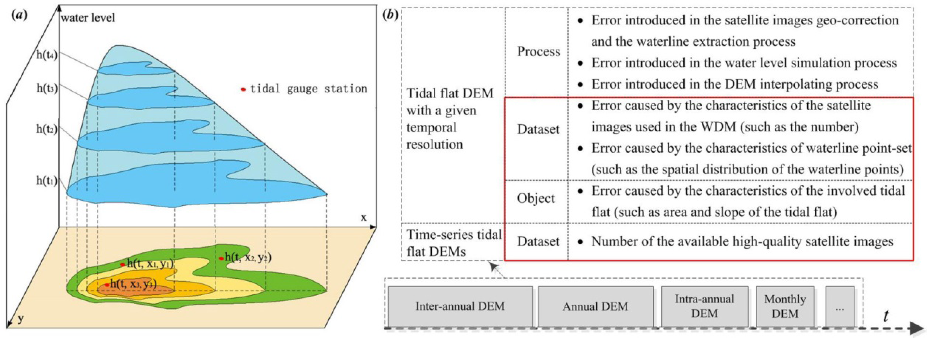
3.1. Rationale of the Waterline Method
- (1)
- Extract the waterlines from the time-series of satellite images. The locations (x, y) of the water-land boundary are extracted from the satellite images.
- (2)
- Simulate the water level at the time of satellite overpass. The water level (h) relative to a datum is calculated from transect data, tide gauge data or a hydraulic model.
- (3)
- Assign a water level to each discrete waterline point. All of the waterlines are discretized to points and are then assigned water levels that correspond to the time of acquisition.
- (4)
- Interpolate the tidal flat DEM. All of the waterline points over a specific period are merged into a waterline-point dataset, and a gridded DEM is created using spatial interpolation techniques.
3.2. Potential Errors in the Waterline Method
- (1)
- a sufficient number of satellite images was taken over a short time period, so the variation in the topography over the tidal flats can be reasonably neglected [20];
- (2)
- high-quality satellite images taken at various water levels were collected and can be used to construct a DEM over a given inter-tidal zone [19];
- (3)
- the waterlines in a given satellite image accurately indicate the water level.
- (1)
- Positional error introduced during the geo-correction and waterline extraction processing of the satellite images. The error introduced in the geo-correction process may result in positional distortion of the waterlines in the satellite images. In most cases, the total root mean square error (RMSE) is less than 0.5 pixels because of the gentle topography in the intertidal zone [15]. Moreover, errors in the positional accuracy may also arise from the waterline extraction process, in which the positional error depends on the waterline extraction method, the band combination, the influence of mixed pixels and other factors. The waterline position can easily be identified in the near-infrared or short-wave infrared bands [34]. Many waterline delineation methods have been proposed based on water’s spectral characteristics in these two bands. However, it is difficult to find an appropriate method to delineate waterlines in multi-source and multi-temporal RS images. Moreover, the study region covers an area of more than 2,100 km2, and the boundary between the water and the tidal flat varies spatially and temporally. To ensure the accuracy of the resultant tidal flat DEMs, on-screen digitization was used instead of automated waterline extraction methods. False-color composite (i.e., near-infrared, red and green spectral bands) are preferred, because they best discern water from other land cover. Specifically, the near-infrared bands include band 4 of the Landsat TM, CBERS-2 CCD, HJ CCD, IRS-P6 and AWiFS/LISS images and band 3 of the SPOT HRV and Beijing-1 CCD images; the red bands include band 3 of the Landsat TM, CBERS-2 CCD, HJ CCD and IRS-P6 AWiFS/LISS images and band 2 of the SPOT HRV and Beijing-1 CCD images; and the green bands include band 2 of the Landsat TM, CBERS-2 CCD, HJ CCD and IRS-P6 AWiFS/LISS images and band 1 of the SPOT HRV and Beijing-1 CCD images. Digitization was performed according to the spectral and spatial characteristics of the tidal flats in the false-color composite images. Waterlines within the internal sandbank around tidal creeks were not considered in the analysis. The average positional error of the extracted waterlines is less than one pixel [17]. Given that the mean slope of a typical intertidal zone ranges between 1‰ and 3‰, the total positional error (1.5 pixels) may result in vertical errors of 4.5–13.5 cm on a 30 m resolution satellite image. Furthermore, the positional error introduced in the geo-correction and waterline extraction of the images and its influence on the accuracy has been discussed in the literature [20,32,35]; hence, this factor is not a focus of this study.
- (2)
- Error introduced in the water level simulation process. The accuracy of the tidal level simulation depends on the complexity of the hydrodynamic conditions, the accuracy of the seafloor topography used in the hydrodynamic model, the characteristics of the simulation method (such as the cell size of the model and the open boundaries) and the accuracy of the calibration data [36]. The error is usually a few tens of centimeters (approximately 10–30 cm) under reasonably calm weather conditions [11,36]. In general, the waterlines can be treated as quasi-contour lines of the topography at a small scale. To apply the waterline method to broader regions, the spatial variation of the water level must be considered. This study covers an area of approximately 35 km × 60 km. A two-dimensional hydraulic model for the South Yellow Sea was constructed using Delft 3D (WL|Delft Hydraulics) to simulate the water level at the satellite overpass times. The average error in the tidal level simulation results is less than 30 cm [15]. Moreover, it is difficult to simulate the regional water level at different accuracies to analyze the relationship between the accuracy of the resultant tidal flat DEM and the accuracy of the water level simulation results. Hence, the vertical error caused by the hydrodynamic model was regarded as constant in the following quantitative error analysis.
- (3)
- Error caused by the distribution of water levels. The distribution of water levels in the satellite images impacts the accuracy of tidal flat DEMs that are based on the waterline method. However, the tidal condition of the study area is complex; two tidal systems, the East China Sea progressive tidal wave and the Southern Yellow Sea rotary tidal wave, converge near the coastal waters of Jianggang [2]. The tide in the study region is not synchronous (especially on the eastern and western sides of the Dongsha Sandbank), so it is difficult to analyze the distribution of the water level and its influence on the accuracy. Hence, the impacts of the distribution of water levels in the satellite images on the accuracy of the tidal flat DEMs are not fully considered in this study.
- (4)
- Error introduced in the DEM interpolation process. This factor is analyzed in Section 4.1.
- (5)
- Error caused by the number of time-series satellite images used in the waterline method. This factor is analyzed in Section 4.2.
- (6)
- Error caused by the distribution of the water level. This factor is analyzed in Section 4.3.
- (7)
- Error caused by the characteristics of the tidal flat (such as area and slope). This factor is analyzed in Section 4.4.
4. Quantitative Analysis Results
4.1. The Spatial Interpolation Approach and Its Impact on the Accuracy
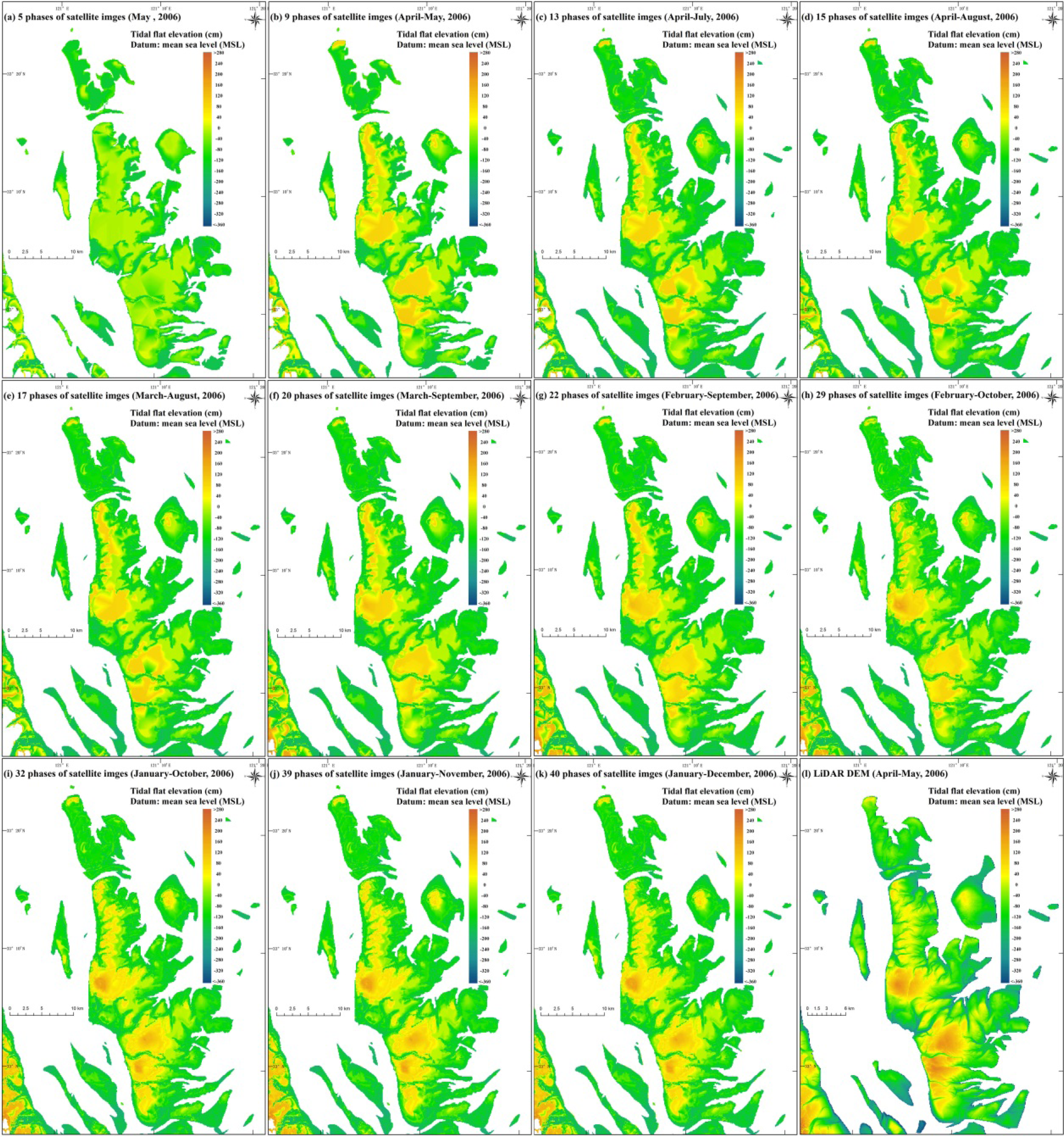
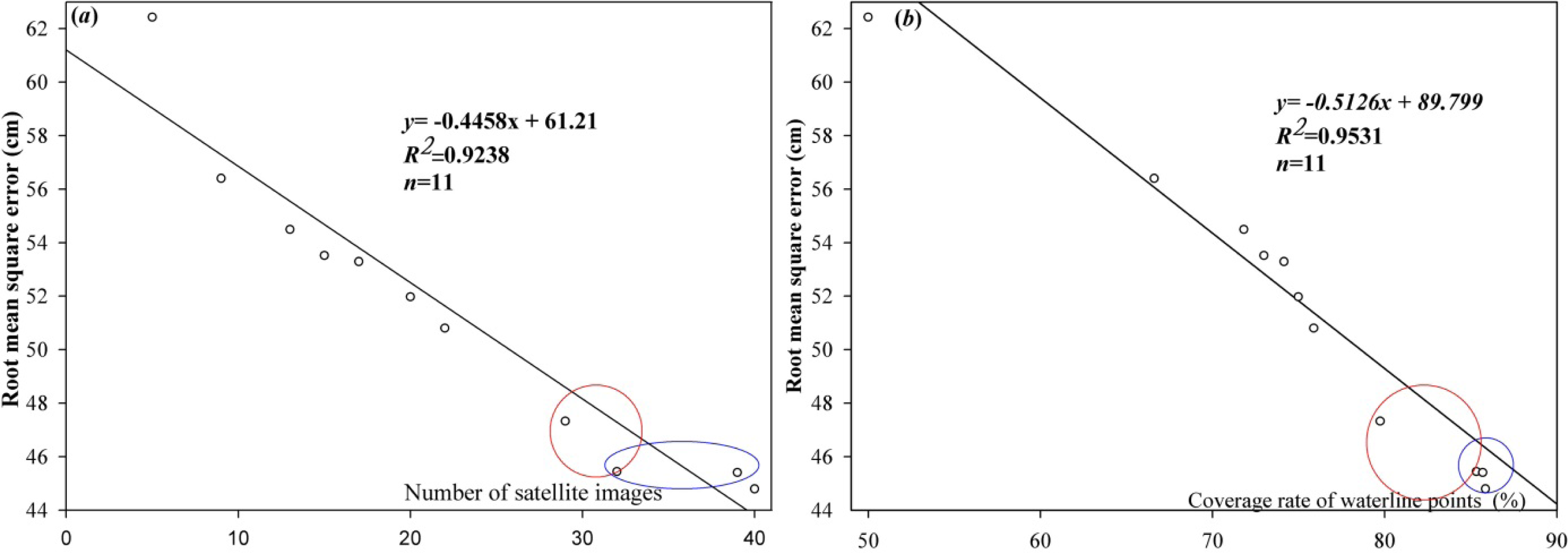
4.2. The Number of Satellite Images Used and Its Impact on the Accuracy
4.3. Characteristics of the Waterline Points and Their Impact on the Accuracy
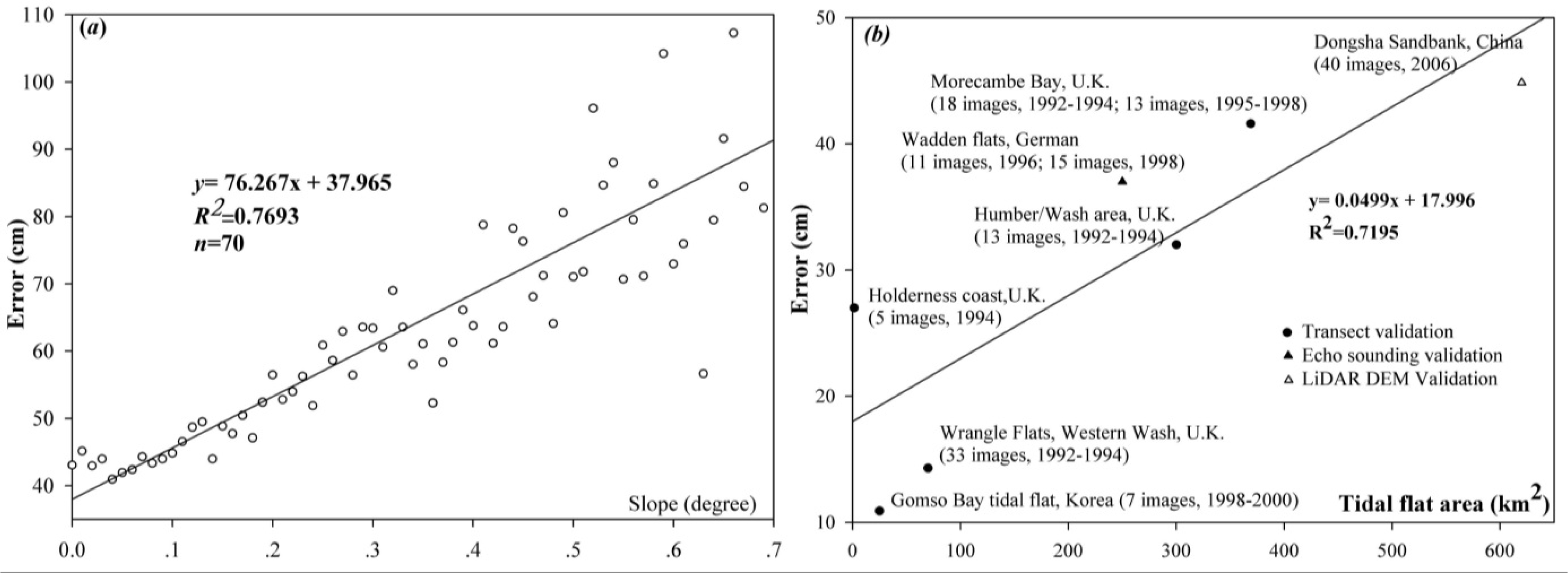
4.4. Characteristics of the Tidal Flats and Their Impact on the Accuracy
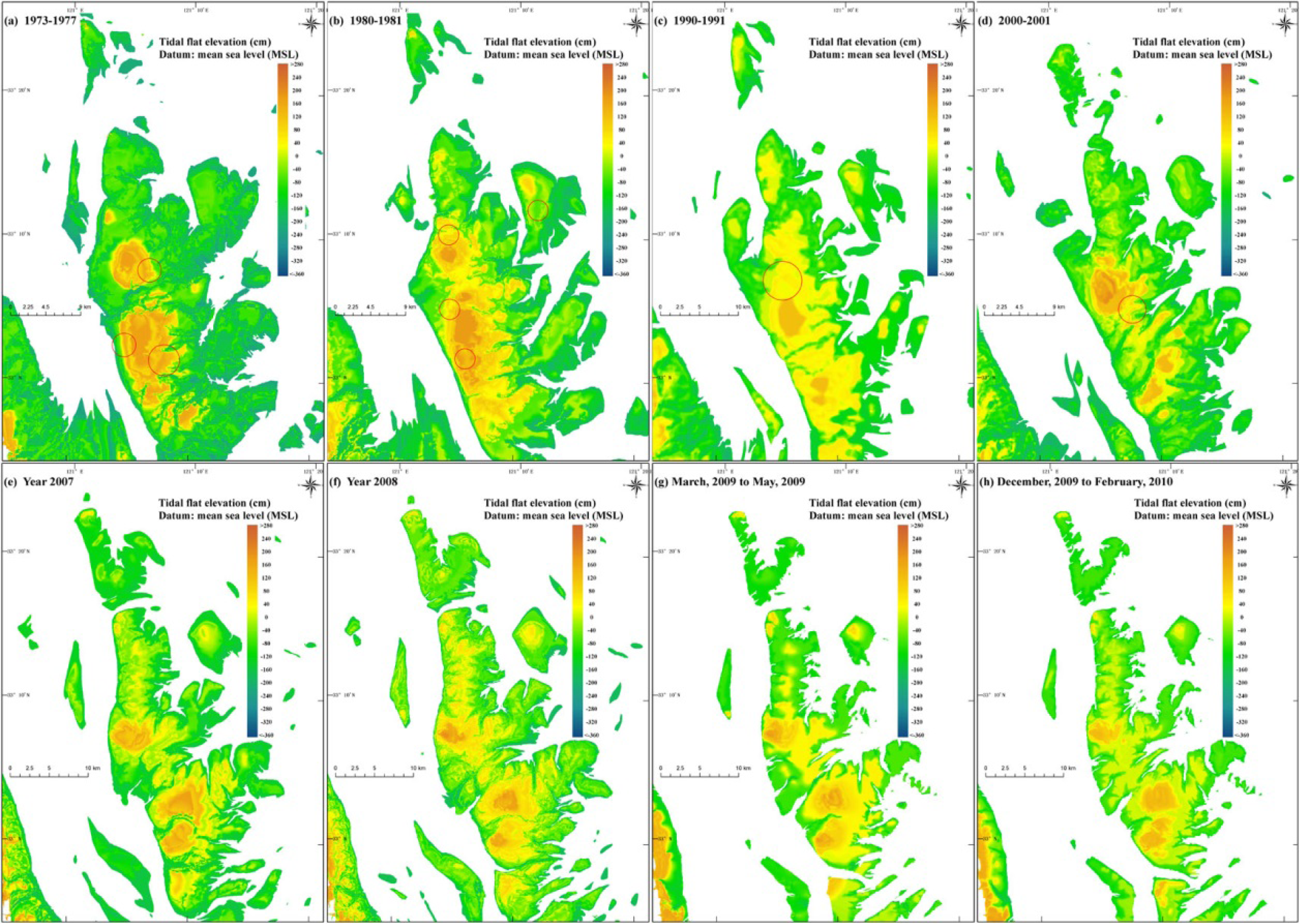
4.5. Potential Temporal Resolution of the Tidal Flat DEM Based on the Waterline Method
5. Conclusions
- (1)
- The number of satellite images used in the waterline method and the coverage rate of the waterline points are statistically correlated with the RMSEs of the resultant DEMs. In particular, the coverage rate of the waterline points is more closely related to the accuracy of the resultant DEMs than the number of images, which implies that increasing the number of satellite images used in the waterline method may only slightly improve the accuracy, while additional waterline points could significantly improve the accuracy of the DEMs.
- (2)
- The area and the slope of the tidal flats reflect the inherent spatial variability of the tidal flats. Tidal flat DEM inversion over a large-scale tidal flat with complex landforms requires denser waterlines and a higher coverage rate to delineate the micro-morphology and to account for regional loss.
- (3)
- The availability analysis of the archive satellite images indicated that the waterline method is able to recover tidal flat terrains from the past forty years. The upper limit of the temporal resolution of the tidal flat DEMs is one year since 1992, half a year since 2004 and three months since 2008, which makes the method practical for research on inter-annual, inter-seasonal or even intra-seasonal trends of tidal flat evolution.
Acknowledgments
Conflicts of Interest
References and Notes
- Chen, J.Y.; Cheng, H.Q.; Dai, Z.J.; Eisma, D. Harmonious development of utilization and protection of tidal flats and wetlands—A case study in Shanghai area. China Ocean Eng 2008, 22, 649–662. [Google Scholar]
- Wang, Y.P.; Gao, S.; Jia, J.J.; Thompson, C.E.L.; Gao, J.H.; Yang, Y. Sediment transport over an accretional intertidal flat with influences of reclamation, Jiangsu coast, China. Mar. Geol 2012, 291, 147–161. [Google Scholar]
- Murray, N.J.; Phinn, S.R.; Clemens, R.S.; Roelfsema, C.M.; Fuller, R.A. Continental scale mapping of tidal flats across East Asia using the Landsat archive. Remote Sens 2012, 4, 3417–3426. [Google Scholar]
- Wimmer, C.; Siegmund, R.; Schwabisch, M.; Moreira, J. Generation of high precision DEMs of the Wadden Sea with airborne interferometric SAR. IEEE Trans. Geosci. Remote Sens 2000, 38, 2234–2245. [Google Scholar]
- Klemas, V. Beach profiling and LIDAR bathymetry: An overview with case studies. J. Coast. Res 2011, 27, 1019–1028. [Google Scholar]
- Sallenger, A.H.; Krabill, W.B.; Swift, R.N.; Brock, J.; List, J.; Hansen, M.; Holman, R.A.; Manizade, S.; Sontag, J.; Meredith, A. etc.. Evaluation of airborne topographic lidar for quantifying beach changes. J. Coast. Res 2003, 19, 125–133. [Google Scholar]
- Mason, D.C.; Gurney, C.; Kennett, M. Beach topography mapping: A comparison of techniques. J. Coast. Conserv 2000, 6, 113–124. [Google Scholar]
- Durbha, S.S.; King, R.L. Semantics-enabled framework for knowledge discovery from earth observation data archives. IEEE Trans. Geosci. Remote Sens 2005, 43, 2563–2572. [Google Scholar]
- Li, Y.K.; Bretschneider, T.R. Semantic-sensitive satellite image retrieval. IEEE Trans. Geosci. Remote Sens 2007, 45, 853–860. [Google Scholar]
- Mason, D.C.; Amin, M.; Davenport, I.J.; Flather, R.A.; Robinson, G.J.; Smith, J.A. Measurement of recent intertidal sediment transport in Morecambe Bay using the waterline method. Estuar. Coast. Shelf Sci 1999, 49, 427–456. [Google Scholar]
- Mason, D.C.; Davenport, I.J.; Flather, R.A.; Gurney, C. A digital elevation model of the inter-tidal areas of the Wash, England, produced by the waterline method. Int. J. Remote Sens 1998, 19, 1455–1460. [Google Scholar]
- Heygster, G.; Dannenberg, J.; Notholt, J. Topographic mapping of the German tidal flats analyzing SAR images with the waterline method. IEEE Trans. Geosci. Remote Sens 2010, 48, 1019–1030. [Google Scholar]
- Anthony, E.J.; Dolique, F.; Gardel, A.; Gratiot, N.; Proisy, C.; Polidori, L. Nearshore intertidal topography and topographic-forcing mechanisms of an Amazon-derived mud bank in French Guiana. Cont. Shelf Res 2008, 28, 813–822. [Google Scholar]
- Baghdadi, N.; Gratiot, N.; Lefebvre, J.P.; Oliveros, C.; Bourguignon, A. Coastline and mudbank monitoring in French Guiana: Contributions of radar and optical satellite imagery. Can. J. Remote Sens 2004, 30, 109–122. [Google Scholar]
- Liu, Y.X.; Li, M.C.; Cheng, L.; Li, F.X.; Chen, K.F. Topographic mapping of offshore sandbank tidal flats using the waterline detection method: A case study on the Dongsha Sandbank of Jiangsu Radial Tidal Sand Ridges, China. Mar. Geod 2012, 35, 362–378. [Google Scholar]
- Liu, Y.X.; Li, M.C.; Cheng, L.; Li, F.X.; Shu, Y.M. A DEM inversion method for inter-tidal zone based on MODIS dataset: A case study in the Dongsha Sandbank of Jiangsu Radial Tidal Sand-Ridges, China. China Ocean Eng 2010, 24, 735–748. [Google Scholar]
- Liu, Y.X.; Li, M.C.; Mao, L.; Cheng, L.; Li, F.X. Toward a method of constructing tidal flat digital elevation models with MODIS and medium-resolution satellite images. J. Coast. Res 2013, 29, 438–448. [Google Scholar]
- Lohani, B.; Mason, D.C. Construction of a digital elevation model of the Holderness coast using the waterline method and airborne thematic mapper data. Int. J. Remote Sens 1999, 20, 593–607. [Google Scholar]
- Niedermeier, A.; Hoja, D.; Lehner, S. Topography and morphodynamics in the German Bight using SAR and optical remote sensing data. Ocean Dyn 2005, 55, 100–109. [Google Scholar]
- Zhao, B.; Guo, H.; Yan, Y.; Wang, Q.; Li, B. A simple waterline approach for tidelands using multi-temporal satellite images: A case study in the Yangtze Delta. Estuar. Coast. Shelf Sci 2008, 77, 134–142. [Google Scholar]
- Ren, M.E.; The, South; Yellow, Sea. Radial Sand Ridges (SYSRSR). In Investigation Report on Jiangsu Tidal Flat and Tidal Resources; (In Chinese); China Ocean Press: Beijing, China, 1985; pp. 164–168. [Google Scholar]
- Zhang, R.S.; Chen, C.J. The Distribution of Modern Offshore Sandbanks in Jiangsu. In Study of the Evolution of Jiangsu Offshore Sandbanks and the Prospects for Tiaozini Sandbanks Merging into Land; (In Chinese); China Ocean Press: Beijing, China, 1992; pp. 23–25. [Google Scholar]
- Zhang, R.S. Equilibrium state of tidal mud flat, a case-coastal area of central Jiangsu, China. Chin. Sci. Bull 1995, 40, 1363–1368. [Google Scholar]
- Zhang, R.S.; Shen, Y.M.; Lu, L.Y.; Yan, S.G.; Wang, Y.H.; Li, J.L.; Zhang, Z.L. Formation of Spartina alterniflora salt marshes on the coast of Jiangsu Province, Spain. Ecol. Eng 2004, 23, 95–105. [Google Scholar]
- Zhang, R.S. Suspended sediment transport processes on tidal mud flat in Jiangsu Province, China. Estuar. Coast. Shelf Sci 1992, 35, 225–233. [Google Scholar]
- Ren, M.E.; Zhang, R.S.; Yang, J.H. Effect of typhoon No.8114 on coastal morphology and sedimentation of Jiangsu Province, People’s Republic of China. J. Coast. Res 1985, 1, 21–28. [Google Scholar]
- Japan Aerospace Exploration Agency. Available online: http://www.eorc.jaxa.jp (accessed on 31 July 2013).
- China Remote Sensing Satellite Ground Station. Available online: http://www.rsgs.ac.cn (accessed on 31 July 2013).
- Remote Sensing Technology Center of Japan. Available online: https://cross.restec.or.jp (accessed on 31 July 2013).
- China Centre for Resources Satellite Data and Application. Available online: http://www.cresda.com (accessed 31 July 2013).
- Beijing Twenty-first Century Science and Technology Development Co., L.B. Available online: http://www.blmit.com.cn (accessed on 31 July 2013).
- Mason, D.C.; Davenport, I.J.; Robinson, G.J.; Flather, R.A.; McCartney, B.S. Construction of an intertidal digital elevation model by the “water-line” method. Geophys. Res. Lett 1995, 22, 3187–3190. [Google Scholar]
- Chen, L.C.; Rau, J.Y. Detection of shoreline changes for tideland areas using multi-temporal satellite images. Int. J. Remote Sens 1998, 19, 3383–3397. [Google Scholar]
- Ryu, J.H.; Won, J.S.; Min, K.D. Waterline extraction from Landsat TM data in a tidal flat—A case study in Gomso Bay, Korea. Remote Sens. Environ 2002, 83, 442–456. [Google Scholar]
- Ryu, J.-H.; Kim, C.-H.; Lee, Y.-K.; Won, J.-S.; Chun, S.-S.; Lee, S. Detecting the intertidal morphologic change using satellite data. Estuari. Coast. Shelf Sci 2008, 78, 623–632. [Google Scholar]
- Chen, K.F.; Wang, Y.H.; Lu, P.D.; Zheng, J.H. Effects of coastline changes on tide system of Yellow Sea off Jiangsu coast, China. China Ocean Eng 2009, 23, 741–750. [Google Scholar]
- Klocke, B. Topographische Karte des Wattenmeeres aus ERS-1 SAR- und Modelldaten; Logos Verlag: Berlin, Germany, 2001; Volume 7. [Google Scholar]
- Wang, Y. Satellite SAR Imagery for Topographic Mapping of the Tidal Flat Areas in the Dutch Wadden Sea; ITC Enschede: Enschede, The Netherlands, 1997; Volume 47. [Google Scholar]
- Mason, D.C.; Davenport, I.J.; Flather, R.A.; Gurney, C.; Robinson, G.J.; Smith, J.A. A sensitivity analysis of the waterline method of constructing a digital elevation model for intertidal areas in ERS SAR scene of eastern England. Estuar. Coast. Shelf Sci 2001, 53, 759–778. [Google Scholar]
- Blott, S.J.; Pye, K. Application of lidar digital terrain modelling to predict intertidal habitat development at a managed retreat site: Abbotts Hall, Essex, UK. Earth Surf. Process. Landf 2004, 29, 893–905. [Google Scholar]
- Mason, D.C.; Scott, T.R.; Dance, S.L. Remote sensing of intertidal morphological change in Morecambe Bay, UK, between 1991 and 2007. Estuar. Coast. Shelf Sci 2010, 87, 487–496. [Google Scholar]
- Liu, Y.; Li, M.; Mao, L.; Cheng, L.; Chen, K. Seasonal pattern of tidal-flat topography along the Jiangsu middle coast, China, using HJ-1 optical images. Wetlands 2013, 33, 871–886. [Google Scholar]


| Satellite | Sensor | Period | High-Quality images | Total RS images | Preview Images Source |
|---|---|---|---|---|---|
| Landsat-1/2/3/4 (USA) | MSS | 1973–11 1998–12 | 136 | 294 | JAXA, http://www.eorc.jaxa.jp [27] |
| Landsat-4/5 (USA) | TM | 1984–05 2011–04 | 194 | 605 | RSGS, http://www.rsgs.ac.cn [28] |
| MOS-1/1b (Japan) | MESSR | 1987–09 1995–11 | 40 | - | RESTEC, https://cross.restec.or.jp [29] |
| JERS-1 (Japan) | SAR | 1992–10 1998–08 | 31 | - | RESTEC, https://cross.restec.or.jp [29] |
| ERS-1/2 (ESA) | SAR | 1995–12 2011–02 | 61 | 65 | RSGS, http://www.rsgs.ac.cn [28] |
| Landsat-7 (USA) | ETM+ | 1999–10 2003–03 | 38 | 63 | RSGS, http://www.rsgs.ac.cn [28] |
| CBERS01/02/02B (China) | CCD | 2000–09 2009–12 | 37 | - | CRESDA, http://www.cresda.com [30] |
| IRS-P6 (India) | AWIFS | 2005–02 2010–10 | 61 | 535 | RSGS, http://www.rsgs.ac.cn [28] |
| Beijing-1 (China) | CCD | 2006–03 2010–06 | 21 | 64 | http://www.blmit.com.cn [31] |
| Envisat (ESA) | ASAR | 2006–01 2010–12 | 55 | - | RSGS, http://www.rsgs.ac.cn [28] |
| HJ-1 A/B CCD (China) | CCD | 2008–10 2010–12 | 178 | 705 | CRESDA, http://www.cresda.com [30] |
| No. | Sensor | Acquisition Time* yyyy-mm-dd hh:mm | Height† (cm) | No. | Sensor | Acquisition Time* yyyy-mm-dd hh:mm | Height† (cm) | No. | Sensor | Acquisition Time* yyyy-mm-dd hh:mm | Height† (cm) |
|---|---|---|---|---|---|---|---|---|---|---|---|
| 1 | Landsat1 MSS | 1973-11-16 02:01 | −154.7 | 78 | Landsat7 ETM+ | 2000-11-28 02:21 | −2.3 | 155 | IRS-P6 AWiFS | 2008-03-24 02:46 | 4.9 |
| 2 | Landsat2 MSS | 1975-03-26 01:52 | 161.2 | 79 | Landsat5 TM | 2000-12-06 02:10 | 34.8 | 156 | CBERS CCD | 2008-04-23 03:07 | 36.9 |
| 3 | Landsat2 MSS | 1975-05-19 01:51 | −78.5 | 80 | Landsat7 ETM+ | 2000-12-14 02:21 | −57.8 | 157 | CBERS CCD | 2008-05-02 02:55 | 88.9 |
| 4 | Landsat2 MSS | 1976-03-20 01:48 | −230.7 | 81 | Landsat5 TM | 2000-12-22 02:10 | 116.7 | 158 | CBERS CCD | 2008-05-05 02:51 | 209.2 |
| 5 | Landsat2 MSS | 1976-04-07 01:47 | −132.5 | 82 | CBERS CCD | 2006-01-10 02:35 | 21.3 | 159 | IRS-P6 AWiFS | 2008-05-06 02:53 | 177.8 |
| 6 | Landsat2 MSS | 1976-04-25 01:47 | 107.3 | 83 | ERS SAR | 2006-01-22 02:33 | −132.5 | 160 | IRS-P6 AWiFS | 2008-05-07 02:33 | 63.7 |
| 7 | Landsat2 MSS | 1976-10-22 01:41 | 171.1 | 84 | IRSP6 LISS3 | 2006-01-27 02:45 | 70.7 | 161 | IRS-P6 AWiFS | 2008-05-11 02:49 | −184.3 |
| 8 | Landsat2 MSS | 1976-11-27 01:40 | −170.8 | 85 | IRSP6 AWiFS | 2006-02-10 02:51 | 68.1 | 162 | CBERS CCD | 2008-05-31 02:52 | 68.0 |
| 9 | Landsat2 MSS | 1976-12-15 01:39 | −48.2 | 86 | ERS SAR | 2006-02-26 02:33 | 122.0 | 163 | CBERS CCD | 2008-06-29 02:48 | 45.1 |
| 10 | Landsat2 MSS | 1977-04-02 01:35 | 127.9 | 87 | CBERS CCD | 2006-03-03 02:33 | −96.7 | 164 | CBERS CCD | 2008-10-08 02:52 | −7.1 |
| 11 | Landsat2 MSS | 1977-04-20 01:34 | −89.7 | 88 | CBERS CCD | 2006-03-29 02:32 | 170.5 | 165 | HJ-1B CCD | 2008-10-17 02:43 | 70.7 |
| 12 | Landsat3 MSS | 1977-07-01 01:30 | 70.4 | 89 | ERS-2 SAR | 2006-04-02 02:33 | −127.6 | 166 | HJ-1A CCD | 2008-10-27 02:50 | 191.9 |
| 13 | Landsat2 MSS | 1977-08-06 01:28 | −121.9 | 90 | BJ-1 CCD | 2006-04-02 02:18 | −155.2 | 167 | HJ-1A CCD | 2008-11-04 02:57 | −61.4 |
| 14 | Landsat2 MSS | 1977-09-29 01:25 | −71.4 | 91 | ERS SAR | 2006-04-17 14:14 | −148.9 | 168 | HJ-1A CCD | 2008-11-12 03:03 | 176.7 |
| 15 | Landsat2 MSS | 1977-10-17 01:24 | −189.4 | 92 | CBERS CCD | 2006-04-24 02:32 | 80.0 | 169 | HJ-1B CCD | 2008-11-21 02:45 | −75.5 |
| 16 | Landsat3 MSS | 1980-05-01 01:45 | −9.1 | 93 | SPOT HRV | 2006-05-03 02:30 | −167 | 170 | CBERS CCD | 2008-11-29 02:52 | 82.4 |
| 17 | Landsat3 MSS | 1980-09-04 01:41 | 70.4 | 94 | IRS-P6 LISS | 2006-05-03 02:45 | −155 | 171 | HJ-1B CCD | 2008-12-07 02:58 | −57.5 |
| 18 | Landsat3 MSS | 1980-10-28 01:39 | −184.9 | 95 | ERS SAR | 2006-05-07 02:33 | −7.4 | 172 | HJ-1B CCD | 2008-12-10 02:36 | 103.3 |
| 19 | Landsat3 MSS | 1980-12-03 01:40 | 106.6 | 96 | BJ-1 CCD | 2006-05-21 02:21 | −92.1 | 173 | HJ-1A CCD | 2008-12-12 02:38 | 155.6 |
| 20 | Landsat2 MSS | 1981-01-17 01:50 | 112.3 | 97 | Landsat5 TM | 2006-05-29 02:23 | 1.4 | 174 | HJ-1B CCD | 2008-12-14 02:39 | 83.8 |
| 21 | Landsat2 MSS | 1981-02-04 01:50 | 72.7 | 98 | ERS SAR | 2006-07-16 02:33 | −193.2 | 175 | HJ-1B CCD | 2008-12-15 03:04 | 52.9 |
| 22 | Landsat3 MSS | 1981-04-26 01:45 | −141.4 | 99 | IRSP6 AWiFS | 2006-07-29 02:33 | −99.8 | 176 | HJ-1A CCD | 2008-12-16 02:41 | −69.1 |
| 23 | Landsat3 MSS | 1981-06-01 01:47 | 177.6 | 100 | SPOT HRV | 2006-07-30 02:38 | −121.3 | 177 | HJ-1B CCD | 2008-12-22 02:45 | −23.0 |
| 24 | Landsat3 MSS | 1981-07-07 01:48 | −197.9 | 101 | BJ-1 CCD | 2006-07-31 02:25 | −138.5 | 178 | HJ-1B CCD | 2009-03-06 02:53 | −79.3 |
| 25 | Landsat3 MSS | 1981-07-25 01:48 | −59.5 | 102 | Landsat5 TM | 2006-08-01 02:23 | −124.4 | 179 | HJ-1B CCD | 2009-03-14 02:59 | −19.3 |
| 26 | Landsat3 MSS | 1981-08-12 01:49 | 117.0 | 103 | ERS SAR | 2006-08-20 02:33 | 123.1 | 180 | HJ-1A CCD | 2009-03-15 02:35 | −132.9 |
| 27 | Landsat2 MSS | 1981-09-08 01:47 | 29.7 | 104 | SPOT HRV | 2006-09-06 02:35 | 197.7 | 181 | HJ-1B CCD | 2009-03-17 02:36 | −168.3 |
| 28 | Landsat3 MSS | 1981-09-17 01:49 | −135.6 | 105 | Landsat5 TM | 2006-09-18 02:24 | 116.6 | 182 | HJ-1B CCD | 2009-03-18 03:02 | −139.0 |
| 29 | Landsat3 MSS | 1981-10-23 01:51 | 112.4 | 106 | ERS SAR | 2006-09-24 02:33 | 65.8 | 183 | HJ-1A CCD | 2009-03-20 03:03 | −68.3 |
| 30 | Landsat3 MSS | 1981-11-10 01:51 | 178.2 | 107 | Landsat5 TM | 2006-10-04 02:24 | 159.5 | 184 | HJ-1A CCD | 2009-03-24 03:06 | 111.4 |
| 31 | Landsat2 MSS | 1981-11-19 01:48 | −67.4 | 108 | SPOT HRV | 2006-10-06 02:31 | 217.8 | 185 | HJ-1B CCD | 2009-03-25 02:42 | 141.2 |
| 32 | Landsat2 MSS | 1981-12-07 01:49 | 84.5 | 109 | BJ-1 CCD | 2006-10-07 02:09 | 161.7 | 186 | HJ-1B CCD | 2009-04-02 02:48 | −183.8 |
| 33 | Landsat2 MSS | 1981-12-25 01:49 | 87.1 | 110 | IRSP6 AWiFS | 2006-10-08 02:55 | 182.4 | 187 | HJ-1B CCD | 2009-04-06 02:51 | 79.4 |
| 34 | Landsat5 TM | 1990-02-26 01:51 | 7.2 | 111 | Landsat5 TM | 2006-10-20 02:24 | 170.2 | 188 | HJ-1A CCD | 2009-04-08 02:53 | 193.7 |
| 35 | MOS1b MESSR | 1990-04-05 02:29 | 10.6 | 112 | IRSP6 AWiFS | 2006-10-27 02:57 | −34.4 | 189 | HJ-1A CCD | 2009-04-15 02:33 | −144.7 |
| 36 | MOS1b MESSR | 1990-05-26 02:32 | 55.6 | 113 | BJ-1 CCD | 2006-10-29 02:10 | −78.6 | 190 | HJ-1B CCD | 2009-04-17 02:35 | −107.5 |
| 37 | Landsat4 TM | 1990-06-02 01:50 | 5.1 | 114 | BJ-1 CCD | 2006-11-01 02:30 | 61.0 | 191 | HJ-1B CCD | 2009-04-18 03:00 | −77.0 |
| 38 | MOS1b MESSR | 1990-07-16 02:34 | −102.9 | 115 | SPOT-4 HRVIR | 2006-11-01 02:31 | 64.8 | 192 | HJ-1B CCD | 2009-04-21 02:38 | 67.1 |
| 39 | Landsat5 TM | 1990-07-20 01:50 | 174.6 | 116 | IRSP6 AWiFS | 2006-11-02 02:33 | 122.8 | 193 | HJ-1B CCD | 2009-04-22 03:03 | 108.3 |
| 40 | Landsat5 TM | 1990-10-08 01:50 | −125.2 | 117 | BJ-1 CCD | 2006-11-03 02:13 | 182.3 | 194 | HJ-1B CCD | 2009-04-25 02:41 | 167.7 |
| 41 | MOS1b MESSR | 1990-10-26 02:38 | −54.0 | 118 | IRSP6 AWiFS | 2006-11-06 02:50 | 183.1 | 195 | HJ-1A CCD | 2009-04-27 02:42 | 49.7 |
| 42 | MOS1b MESSR | 1990-11-12 02:38 | 26.4 | 119 | BJ-1 CCD | 2006-11-15 02:04 | 56.0 | 196 | HJ-1B CCD | 2009-04-29 02:44 | −117.2 |
| 43 | MOS1 MESSR | 1990-12-24 02:42 | −140.0 | 120 | ERS SAR | 2006-12-03 02:33 | 159.0 | 197 | HJ-1A CCD | 2009-05-01 02:45 | −187.7 |
| 44 | MOS1 MESSR | 1991-01-27 02:42 | 40.6 | 121 | Landsat5 TM | 2006-12-23 02:25 | −25.9 | 198 | HJ-1A CCD | 2009-05-05 02:48 | 66.9 |
| 45 | MOS1b MESSR | 1991-02-05 02:41 | −191.3 | 122 | IRS-P6 AWiFS | 2007-01-07 02:58 | −59.6 | 199 | HJ-1B CCD | 2009-05-07 02:50 | 184.7 |
| 46 | Landsat5 TM | 1991-04-02 01:52 | −128.5 | 123 | CBERS CCD | 2007-01-09 02:25 | −155.9 | 200 | HJ-1A CCD | 2009-05-09 02:51 | 171.2 |
| 47 | Landsat5 TM | 1991-07-23 01:54 | 119.9 | 124 | ERS2 SAR | 2007-01-26 02:35 | −186.2 | 201 | HJ-1B CCD | 2009-05-11 02:53 | 53.3 |
| 48 | Landsat5 TM | 1991-08-24 01:54 | 116.7 | 125 | IRS-P6 AWiFS | 2007-01-27 02:42 | −141.9 | 202 | HJ-1A CCD | 2009-05-13 02:54 | −66.6 |
| 49 | MOS1b MESSR | 1991-09-14 02:46 | −108.6 | 126 | IRS-P6 AWiFS | 2007-01-31 02:58 | 98.6 | 203 | HJ-1B CCD | 2009-05-18 02:34 | −55.9 |
| 50 | MOS1b MESSR | 1991-09-14 02:46 | −108.6 | 127 | IRS-P6 AWiFS | 2007-03-11 02:46 | −140.4 | 204 | HJ-1B CCD | 2009-05-22 02:36 | 154.6 |
| 51 | Landsat5 TM | 1991-10-11 01:54 | −85.9 | 128 | IRS-P6 AWiFS | 2007-03-20 02:58 | 140.8 | 205 | HJ-1A CCD | 2009-05-24 02:37 | 183.4 |
| 52 | MOS1b MESSR | 1991-10-18 02:47 | 45.7 | 129 | IRS-P6 AWiFS | 2007-03-21 02:38 | 22.4 | 206 | HJ-1B CCD | 2009-05-26 02:39 | 68.6 |
| 53 | Landsat5 TM | 1991-11-28 01:54 | −143.8 | 130 | CBERS CCD | 2007-03-28 02:22 | −17.3 | 207 | HJ-1B CCD | 2009-12-03 02:52 | 136.1 |
| 54 | Landsat7 ETM+ | 2000-01-29 02:23 | −100.2 | 131 | IRS-P6 LISS3 | 2007-04-04 02:47 | 64.2 | 208 | HJ-1B CCD | 2009-12-05 02:52 | 14.9 |
| 55 | Landsat5 TM | 2000-02-06 02:04 | 13.3 | 132 | IRS-P6 LISS3 | 2007-04-09 02:43 | −134.0 | 209 | HJ-1B CCD | 2009-12-07 02:55 | −124.4 |
| 56 | Landsat5 TM | 2000-02-22 02:04 | −109.3 | 133 | IRS-P6 AWiFS | 2007-04-13 02:59 | 1.3 | 210 | HJ-1B CCD | 2009-12-19 03:03 | 19.4 |
| 57 | Landsat7 ETM+ | 2000-03-01 02:23 | 11.1 | 134 | IRS-P6 AWiFS | 2007-04-18 02:54 | 177.6 | 211 | HJ-1A CCD | 2009-12-20 02:38 | −65.9 |
| 58 | Landsat5 TM | 2000-03-09 02:04 | −124.1 | 135 | IRS-P6 AWiFS | 2007-04-23 02:50 | −177.2 | 212 | HJ-1A CCD | 2009-12-21 03:03 | −75.1 |
| 59 | Landsat5 TM | 2000-04-10 02:05 | −215.7 | 136 | IRS-P6 AWiFS | 2007-05-08 02:37 | −140.1 | 213 | HJ-1B CCD | 2009-12-22 02:41 | −122.4 |
| 60 | Landsat5 TM | 2000-04-26 02:06 | −109.1 | 137 | ERS-2 SAR | 2007-05-11 02:35 | −67.4 | 214 | CBERS CCD | 2009-12-22 02:56 | −111.9 |
| 61 | Landsat5 ETM+ | 2000-05-04 02:23 | 144.5 | 138 | CBERS CCD | 2007-06-17 02:14 | −28.0 | 215 | ERS SAR | 2009-12-27 02:35 | −14.4 |
| 62 | Landsat5 TM | 2000-05-12 02:06 | −56.4 | 139 | ERS-2 SAR | 2007-08-05 02:30 | −177.3 | 216 | HJ-1A CCD | 2009-12-28 02:43 | 25.0 |
| 63 | Landsat7 ETM+ | 2000-05-20 02:22 | −5.8 | 140 | IRS-P6 AWiFS | 2007-09-04 02:42 | −128.6 | 217 | HJ-1B CCD | 2009-12-30 02:46 | 111.9 |
| 64 | Landsat5 TM | 2000-05-28 02:06 | 8.2 | 141 | ERS-2 SAR | 2007-09-09 02:32 | 185.9 | 218 | HJ-1A CCD | 2010-01-01 02:46 | 133.5 |
| 65 | Landsat7 ETM+ | 2000-06-05 02:22 | −73.5 | 142 | ERS-2 SAR | 2007-10-14 02:30 | 9.2 | 219 | HJ-1B CCD | 2010-01-03 02:49 | 30.0 |
| 66 | Landsat5 TM | 2000-06-13 02:07 | 135 | 143 | IRS-P6 LISS3 | 2007-11-06 02:46 | 120.8 | 220 | HJ-1A CCD | 2010-01-13 02:54 | 70.5 |
| 67 | Landsat7 ETM+ | 2000-07-07 02:22 | −207.7 | 144 | IRSP6 AWiFS | 2007-11-11 02:40 | 97.6 | 221 | HJ-1B CCD | 2010-01-14 02:32 | 112.3 |
| 68 | Landsat5 TM | 2000-07-31 02:08 | 134.7 | 145 | IRS-P6 AWIFS | 2007-11-21 02:32 | 97.9 | 222 | Landsat5 TM | 2010-01-16 02:22 | 95.6 |
| 69 | Terra AST | 2000-08-01 02:56 | 148.4 | 146 | CBERS CCD | 2007-11-28 02:00 | −115.1 | 223 | HJ-1B CCD | 2010-01-18 02:34 | 11.5 |
| 70 | Landsat5 TM | 2000-09-01 02:08 | −89.1 | 147 | IRS-P6 LISS3 | 2007-11-30 02:45 | −133.9 | 224 | HJ-1A CCD | 2010-01-24 02:36 | −175.8 |
| 71 | Landsat7 ETM+ | 2000-09-09 02:21 | 91.9 | 148 | IRS-P6 AWiFS | 2007-12-15 02:32 | −122.7 | 225 | HJ-1B CCD | 2010-01-26 02:40 | −92.5 |
| 72 | CBERS CCD | 2000-09-16 02:46 | 44.3 | 149 | IRS-P6 AWiFS | 2008-01-02 02:56 | −68.5 | 226 | HJ-1A CCD | 2010-01-28 02:39 | 50.8 |
| 73 | Landsat5 TM | 2000-09-17 02:09 | −92.6 | 150 | IRS-P6 LISS3 | 2008-02-10 02:45 | −47.2 | 227 | HJ-1A CCD | 2010-01-29 03:04 | 86.3 |
| 74 | Landsat5 TM | 2000-10-03 02:09 | −142.7 | 151 | CBERS CCD | 2008-02-17 02:51 | −12.4 | 228 | ERS SAR | 2010-01-31 02:35 | 60.2 |
| 75 | Landsat5 TM | 2000-11-04 02:09 | −43.1 | 152 | IRSP6 LISS3 | 2008-03-05 02:44 | 90.0 | 229 | HJ-1A CCD | 2010-02-05 02:44 | −232.7 |
| 76 | Landsat7 ETM+ | 2000-11-12 02:21 | 136.0 | 153 | IRS-P6 AWiFS | 2008-03-10 02:39 | −11.5 | 230 | HJ-1B CCD | 2010-02-19 02:55 | −103.7 |
| 77 | Landsat5 TM | 2000-11-20 02:09 | −6.6 | 154 | CBERS CCD | 2008-03-14 02:51 | −196.9 | 231 | HJ-1A CCD | 2010-02-21 02:54 | −172.3 |
© 2013 by the authors; licensee MDPI, Basel, Switzerland This article is an open access article distributed under the terms and conditions of the Creative Commons Attribution license ( http://creativecommons.org/licenses/by/3.0/).
Share and Cite
Liu, Y.; Li, M.; Zhou, M.; Yang, K.; Mao, L. Quantitative Analysis of the Waterline Method for Topographical Mapping of Tidal Flats: A Case Study in the Dongsha Sandbank, China. Remote Sens. 2013, 5, 6138-6158. https://doi.org/10.3390/rs5116138
Liu Y, Li M, Zhou M, Yang K, Mao L. Quantitative Analysis of the Waterline Method for Topographical Mapping of Tidal Flats: A Case Study in the Dongsha Sandbank, China. Remote Sensing. 2013; 5(11):6138-6158. https://doi.org/10.3390/rs5116138
Chicago/Turabian StyleLiu, Yongxue, Manchun Li, Minxi Zhou, Kang Yang, and Liang Mao. 2013. "Quantitative Analysis of the Waterline Method for Topographical Mapping of Tidal Flats: A Case Study in the Dongsha Sandbank, China" Remote Sensing 5, no. 11: 6138-6158. https://doi.org/10.3390/rs5116138