1. Introduction
The authors have been exploring a new approach for measuring greenhouse gases (GHG) using Laser Absorption Spectroscopy (LAS) in an open-path configuration [
1]. This new approach has the potential to enable GHG measurement from a transmitter in a geostationary orbit to a network of ground receivers. This approach complements other existing and planned approaches by providing high accuracy near-continuous measurements along a fixed column, which would enable a thorough evaluation of potential bias. This new approach also can be implemented for ground-to-ground applications which are currently unaddressed by available
in situ and remote methods, specifically where measurements are desired over a long path and in the presence of high aerosol content. Used in conjunction with existing methods, these new measurement approaches will provide the precisions required for distinguishing anthropogenic sources from biogenic sources and sinks on regional and local scales.
The Laser Atmospheric Transmitter Receiver-Network (LAnTeRN) concept is an extension of the Exelis-developed Multifunctional Fiber Laser Lidar (MFLL) [
2–
5]. MFLL was developed in 2004 as an airborne demonstration unit for a unique intensity-modulated continuous wave (IM-CW) lidar to actively measure integrated column amounts of atmospheric CO
2 and O
2. The MFLL system relies on low-power, high-reliability telecom laser components to implement a robust and flexible instrument. The MFLL has been extensively evaluated over 13 flight campaigns on three different aircraft by NASA LaRC and our partners at Atmospheric and Environmental Research Inc. (AER). The results show the instrument’s ability to measure CO
2 and O
2 to accuracies approaching those required for the National Research Council’s Active Sensing of CO
2 Emissions over Nights, Days and Seasons (ASCENDS) mission [
6].
LAnTeRN has several fundamental characteristics in common with the MFLL instrument (e.g., an all fiber-coupled, high efficiency transmitter and utilization of the IM-CW approach), but is a fundamentally different implementation with distinct capability. The key difference is that LAnTeRN nominally operates in transmission rather than in the traditional backscatter lidar configuration, which has several distinct advantages.
Operating in transmission offers the following benefits: (1) Eliminates partial path returns from clouds and aerosols as a source of bias which is a key requirement for climate data and other applications, e.g., volcano or forest fire monitoring, where large aerosol concentrations are present; (2) Significantly reduces instrument complexity and data volumes through the use of simple pure sine wave modulation and lock-in amplifier techniques; (3) Enables lower powers and smaller apertures because there is no loss of signal due to reflectance and broad scattering angles; (4) Eliminates the need for companion estimates of surface pressure derived either from model data or remotely sensed measurements to estimate dry air mole fractions, which is a big challenge for ASCENDS, due to the fact that surface pressure and geo-location information can be collected at the receiver; and (5) Reduces cost and risk for a space implementation by keeping the receivers and data collection on the ground, and thus eliminates the need to launch a large telescope and multiple high power transmitters required for ASCENDS.
Furthermore, making the measurement along fixed paths has the following benefits: (1) For a space-based implementation it facilitates extensive validation and calibration options (e.g., aircraft, in situ towers, radiosonde launches, NOAA’s AirCore, etc.) which is very difficult to do with current and planned satellite missions for GHG monitoring to the precision needed for separating biogenic and anthropogenic sources; (2) It provides significant improvements in precision and accuracy for regional monitoring due to the long time series of measurements, both day and night, enabling measurement accuracies through averaging to levels required to separate anthropogenic sources from biogenic sources and sinks; (3) It enables cross calibration opportunities among receivers that are along the same atmospheric path simultaneously and illuminated by the same transmitter, due to the ability to relocate the receivers; (4) For a ground-based implementation it provides direct measurement of GHG time-varying fields and be used to directly measure flux over large areas and long path lengths.
Although several other open path techniques exist [
7–
14], LAnTeRN is a different implementation which simultaneously transmits and receives both the on and the offline wavelengths. This key difference makes many of the noise sources including scintillation common to both wavelengths and since this is a ratiometric measurement they cancel in the ratio. For the more traditional lidar case of MFLL this approach also reduces impacts of varying surface reflectance as well. We believe this is a significant benefit to this measurement approach relative to other common open-path approaches, such as tunable diode laser absorption spectroscopy (TDLAS). In 2011 and 2012, Exelis developed a proof-of-concept demonstration of a LAnTeRN transmitter and receiver pair. The system was designed to demonstrate the ability to build separate transmitter and receivers capable of maintaining sufficiently accurate timing to enable long integration times; to validate a high-fidelity performance model, leveraged from an optical communications model developed by Exelis in a prior effort; and to demonstrate the measurement at power levels predicted for a geostationary implementation. The theory, model description, a description of the instrument, results from experiments performed, and some potential applications of the measurement approach are presented in the following sections.
2. Theory
The LAnTeRN measurement leverages more than a decade of prior work by Exelis Inc. (formerly ITT Exelis Corp.) on the MFLL airborne engineering development unit. The initial implementation of MFLL used pure sinusoidal modulation with each channel (wavelength) having a unique amplitude modulation frequency applied to each. This approach worked very well in the absence of signal returns from intermediate scatterers. However, in the presence of clouds or heavy aerosols, the CW measurement was unable to distinguish the return from the target of interest and those from the intermediate scattering sources. In order to address this for the ASCENDS mission we developed a chirped waveform which enables us to distinguish the return signal from different ranges. Although this approach has worked quite well, these more complicated waveforms significantly increased the cost and complexity of the design through higher bandwidth requirements, large data volumes, and significant computational resources required to post process the data. Additionally, the increased bandwidth can have a negative impact on the instrument SNR performance. The desire to maintain the advantages of the original implementation of MFLL, while developing this more complex approach for the ASCENDS mission, led Exelis to the development of the LAnTeRN concept [
15].
2.1. Application of the Lock-in Amplifier
As mentioned, the LAnTeRN measurement concept enables the use of pure sinusoidal modulations with standard lock-in techniques even in the presence of intermediate scattering media, due to the fact that the measurement is made in transmission. In order to describe the LAnTeRN measurement we will first describe how the signals are encoded, combined prior to transmission, simultaneously received, and then separated through a digital lock-in approach.
The time varying output signal amplitude for wavelength
λm, is represented mathematically by:
where
Am is the signal amplitude,
fm is the modulation frequency, and
θm is the initial phase. Note that this is an amplitude modulation and that the wavelength
λm is held fixed. After applying a unique amplitude modulation scheme to each wavelength in the system, the signals are then combined using fiber combiners prior to transmission into the atmosphere. This is made possible by the fact that both the laser and the modulator are telecom-style fiber coupled components. The resulting output of the system is the sum of
N waveforms, each with a unique wavelength of light and unique amplitude modulation frequency as shown in
Equation (2).
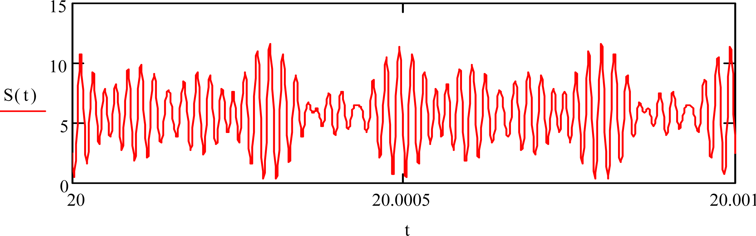
An example of the amplitude of the output signal with
N = 3 is shown in
Figure 1, neglecting noise. For the sake of the discussion we will ignore the effects of the atmosphere and instrument at this time and focus on the lock-in technique for separating the simultaneously transmitted/received wavelengths.
The received optical signal, the transmitted power attenuated by the atmospheric state over the path between the transmit and receive telescopes, is converted into a voltage and recorded using a high-quality Analog-to-Digital Converter (ADC). The amplitude of the received signal at wavelength
λm can then be determined through a standard lock-in approach [
16] based on the knowledge of the frequencies used to modulate the waveforms. A brief description of the well-known lock-in approach is given here for clarity, but, for simplicity, we are not including the discrete nature of the signal after the ADC and the digitally-generated local oscillator signal. The difference in the discrete case is that the lock-in is performed on a sample-by-sample basis by multiplying the sampled signal with a discrete version of the local oscillator signal used to generate the amplitude-modulated output.
To separate out the relative amplitudes of each of the transmitted wavelengths, the received signal is multiplied by both a sine wave and a cosine wave at frequency
fm to determine the in-phase,
I, and out-of-phase,
Q components. Determining both of these components and adding them in quadrature renders the system insensitive to phase variations between the local oscillator signal and the received signal.
The
I and
Q components consist of two AC signals, which oscillate at both the sum and the difference of the signal frequencies and the local oscillator frequency. Taking the time average of these AC signals comes out to zero unless the signal contains a frequency component at the local oscillator frequency
fm. In that case, the time average results in a DC component proportional to the signal amplitude at frequency
fm as the difference frequency approaches zero, and essentially eliminates any signal at frequencies that are not very close to
fm. The bandwidth of the lock-in response around the desired frequency
fm is determined by the length of the time average and is approximately proportional to 1/
t,
i.e., a lock-in period of 1 s results in a contribution to the DC component over a bandwidth of approximately 1 Hz. In the ideal case of an infinite sine wave with an infinite lock-in period, the response is a delta function at frequency
fm. In practice, the frequency response is described by (sin(
x)/
x)
2, known as a sinc
2 function. This is important when selecting the frequencies for each of the channels. Optimally, the frequencies should be spaced such that one frequency is at a minimum of the sinc
2 functions of the other channels while keeping them as close as possible to minimize the impacts of variations in receiver gain characteristics. The time averaged
I and
Q components are then added in quadrature to retrieve the magnitude of the desired signal amplitude as,
The factor of 2 is due to the fact that the lock-in method results in 1/2 of the actual amplitude when
AL equals unity, but since the multiplications from
Equations (3) and
(4) are done digitally, the amplitude of the reference sine wave
AL can be selected arbitrarily. In this example,
AL is selected to be 2, giving the actual amplitude of the mth channel. This is repeated for each of the
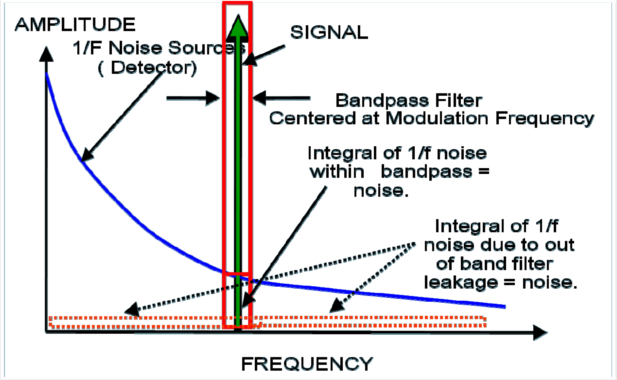
N channels. The beauty of the lock-in amplifier is that it is relatively insensitive to broadband noise, since the output of the time-averaged
I and
Q components is only sensitive to noise at the frequency used for the sine and cosine multiplications as illustrated in
Figure 2. Frequencies are chosen to avoid the typical 1/
f noise and exhibit constant system gain. An analog bandpass filter is used to limit the broadband noise outside of the range of frequencies selected for the N channels, and to avoid aliasing in the ADC.
2.2. Differential Absorption Measurement in Transmissionversus Reflection
Differential absorption techniques for measuring atmospheric gases began appearing shortly after the advent of the laser. The literature describing these various approaches is vast and spans both ground and space concepts. A good general reference can be found in [
17] and a few additional selected examples for the interested reader can be found in references [
18–
24]. Only a brief overview of the concepts is provided here, as needed for clarification of the LAnTeRN measurement concept.
Starting with the standard lidar equation for the received signal power
Prec at wavelength
λ0 from a volumetric scattering target of Δ
R, centered at range
R, given by:
where
PL is the transmitted laser power,
Arec/
R2 is the solid angle subtended by the receiver,
η(
λ0) is the optical efficiency of the receiver system at
λ0,
ξ(
R) is a geometric factor describing the overlap of the laser and the receiver telescope as a function of range,
βπ(
λ0,
R) is the atmospheric volumetric backscatter coefficient at range
R for wavelength
λ0, and is assumed to be homogenous over a slice of the atmosphere of thickness
ΔR centered at
R, and
κ(
λ0,
r) is the volumetric extinction coefficient which is integrated from 0 to range
R and includes both absorption and scattering into angles other than the receiver view angle,
θ ≠ 180° for this standard lidar description. The factor of 2 in the exponent is based on a standard lidar making the measurement in reflection and accounts for the round trip attenuation.
For the case of the LAnTeRN arrangement the standard lidar equation in
Equation (6) can be simplified to,
where we have assumed the area of the transmitted laser signal at range
R (
ALas(
r)) overfills the receiver aperture. The received power is only dependent on the power density at the receiver, the receiver area, the receiver efficiency, and the one-way atmospheric extinction between the transmitter and receiver. By selecting two closely spaced (<100 pm) wavelengths corresponding to an online and offline wavelength, where online refers to a wavelength with significant absorption by the gas of interest and offline refers to a wavelength with much less absorption by the gas of interest, one can apply the standard differential absorption (DA)technique.
where,
is the differential transmission between the online and offline wavelengths to range
R, from the Beer-Lambert law. The DA technique relies on an assumption that the wavelength dependence of the extinction term, both for scattering and absorption, from all but the molecule of interest is negligible. This is a reasonable assumption given the close spacing of the online and offline wavelengths and proper selection of the wavelengths relative to other interfering absorption features. Using this assumption we get the result on the right hand side of
Equation (8) where the general extinction coefficient,
κ, is replaced by the absorption coefficient of the molecule of interest,
α.
By accurately monitoring the transmitted power for both the online and offline signals,
is a known value, and the measurement provides the differential transmission due to the molecule of interest. By taking the natural logarithm of the differential transmission, one is left with the differential absorption,
, which is related to the total column abundance of the gas between the transmitter and receiver, separated by range
R, by:
where Δ
σ(
λon,
λoff,
r) is the differential cross-section between
λon and
λoff as a function of range to range
R, determined through laboratory spectroscopy, and the quantity on the right hand side is the measured value as described above. In reality, Δ
σ is a function of atmospheric pressure, temperature, and water vapor concentration in the path of integration, and thus these parameters must also be quantified in order to determine the effective differential cross-section and derive the dry-air mixing ratios of desired GHGs [
25]. In the LAnTeRN instrument concept, we use coincident
in situ measurements of these meteorological parameters to minimize the atmospheric state uncertainties on determination of Δ
σ, and for the retrieval of the GHG mixing ratio from the average number density.
2.3. Performance Model
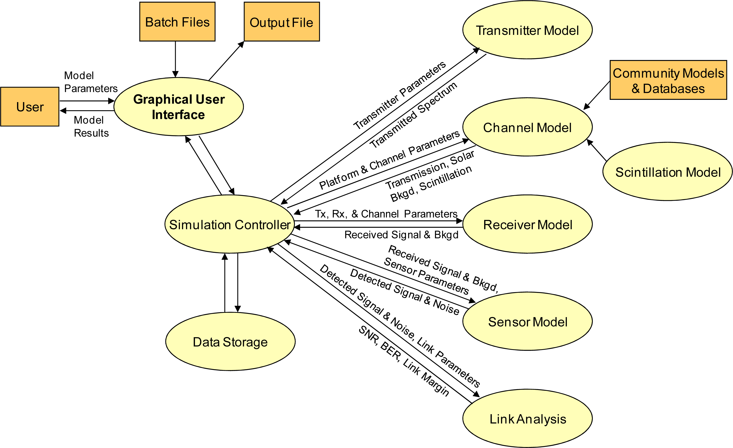
The LAnTeRN performance model was developed by leveraging extensive prior Exelis modeling efforts for point-to-point optical communications systems. A graphical representation of the model is shown in
Figure 3. The model simulates the system performance over a wide range of configurations and environmental conditions and is capable of simulating space-to-ground, airborne-to-ground, and ground-to-ground links. The block diagram shows how the simulation controller interfaces with five separate models to characterize system performance.
Transfer Model (LBLRTM) [
26] to simulate high-resolution atmospheric transmission spectra and Betaspec/LOWTRAN to calculate aerosol extinction. The background solar radiance is calculated from MODTRAN [
27,
28] and allows for day and night performance estimates. In addition, the effects of atmospheric scintillation on beam propagation are calculated using the Andrews and Phillips formulations [
29,
30]. Presently, the model is limited to operating between 1.25 μm and 1.68 μm. Transmitter and receiver locations are specified in three-dimensional space on a WGS-84 ellipsoid [
31], thus, model predictions can be made for specific test sites.
The receiver model calculates the resulting signal and background spectra at the aft end of the receiver optics and then passes them to the sensor module, which contains high-fidelity models of the photodiode detector, transimpedance amplifier (TIA) noise, and lock-in amplifier. All outputs are then fed into the link analysis model that calculates the final system SNR, a link budget, and other signal quality parameters, including individual noise source contributions.
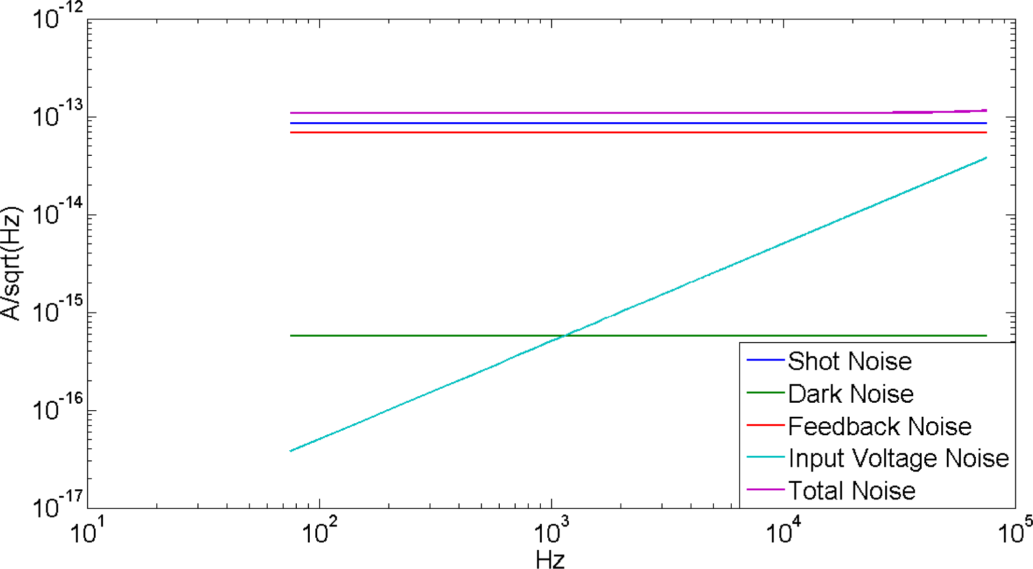
The detector and TIA noise is composed of several noise components. The total electronic current noise in units of
is given by,
Idark is the dark noise associated with a photodetector that has a dynamic impedance of
R0 (Ω) and a temperature of
Tdet (K). Boltzmann’s constant
k is 1.3807e−23 (J/K).
Ishot is the shot noise associated with a photodetector given a DC photocurrent (
IDC), optical gain (
M), and excess noise factor (
Fnoise). The elementary charge (
q) is 1.6022e−19 (C).
The DC photocurrent is a sum of all the photocurrent (A) reaching the device, given by,
Isignal is the photocurrent generated by the source laser, Isolar is the photocurrent generated from the solar radiance that passes through the optical bandpass filter, and Ileakage is the leakage current of the detector as measured by I–V traces of the device.
Iinput_V is the current noise associated with the TIA voltage input noise.
en is the TIA voltage input noise, and
ZD is the detector reactance, defined as,
f is the frequency of interest (Hz), and
Cdet is the detector and cable capacitance (F) to the input of the TIA.
Ifb is the current noise associated with the feedback resistor of the TIA.
Tfb is the temperature of the TIA feedback resistor (K), and
Rfb is the value of the feedback resistor (Ω).
To get total voltage noise at the output of the TIA, the total current noise is multiplied by the transimpedance gain.
where,
Itotal is given by
Equation (10), and
Zf is given by,
An example plot of the noise spectrum for the various model parameters related to the detector and TIA is shown in
Figure 4. These simulated noise terms are combined with those caused by atmospheric effects to produce a total simulated system noise.
The model results were used to predict the performance of the LAnTeRN proof-of-concept system under conditions that would be encountered in the field-testing of the system. These predictions and the measurements made in the field are compared in Section 3.2. Although the model is fairly robust in its present state, it still requires further development. For example, it only considers the laser linewidth, but does not currently model additional noise from the laser source due to wavelength instability. The instrument is robust against other noise sources from the laser such as relative intensity noise due to the lock-in amplifier approach rejecting noise outside of the frequency bandwidth of the lock-in.
3. Instrument Description
The LAnTeRN proof-of-concept instrument is composed of two assemblies, the transmitter (Tx) and the receiver (Rx). The construction of each is very similar, consisting of a rigid plastic enclosure with an attached mast pole. The mast pole is topped with Tx/Rx optics and Wi-Fi antennas.
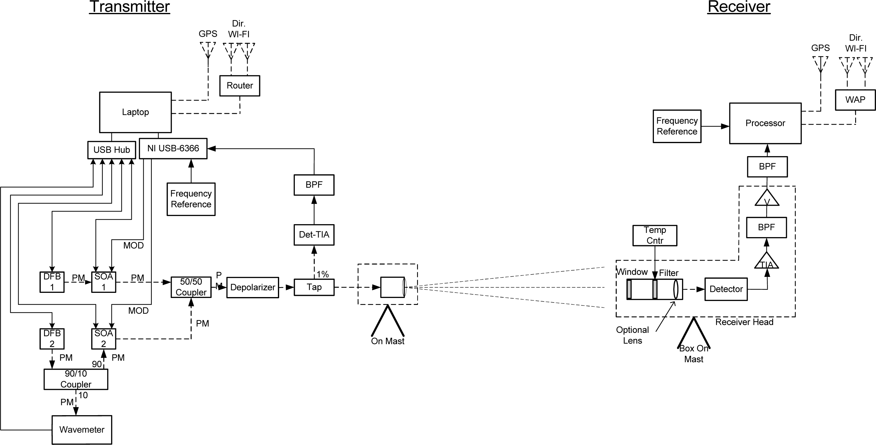
The system block diagram is shown in
Figure 5, and the proof-of-concept instrument specifications are given in
Table 1. The Tx consists of two stable DFB laser wavelength sources (online and offline) with precise current and temperature control, capable of maintaining the wavelengths to <±0.2 pm. Each wavelength is amplified and individually modulated by semiconductor optical amplifiers (SOA). These sources are combined and then transmitted through a single fiber to the mast. An in-line tap couples a portion of the transmitted signal to a reference detector. That electrical signal is amplified, filtered, and then digitized by the processor. A software lock-in function decodes the transmitted amplitudes by detecting their respected modulation tones.
The Tx combined signal is sent toward the Rx from a simple open fiber as a broad-angle beam. Using a wider beam angle minimizes the aiming accuracy required. After passing through the atmosphere the light is received by the Rx, which has a field-of-view approximately equal to that of the Tx.
Using commercial optics and a narrow-band optical filter (BPF), the Rx focuses the signal on an InGaAs detector whose electrical output is then amplified and filtered. The Rx processor digitizes the amplified signal, decodes the digitized signal using a lock-in function with a stable frequency reference, and saves the resulting output data from the lock-in to file.
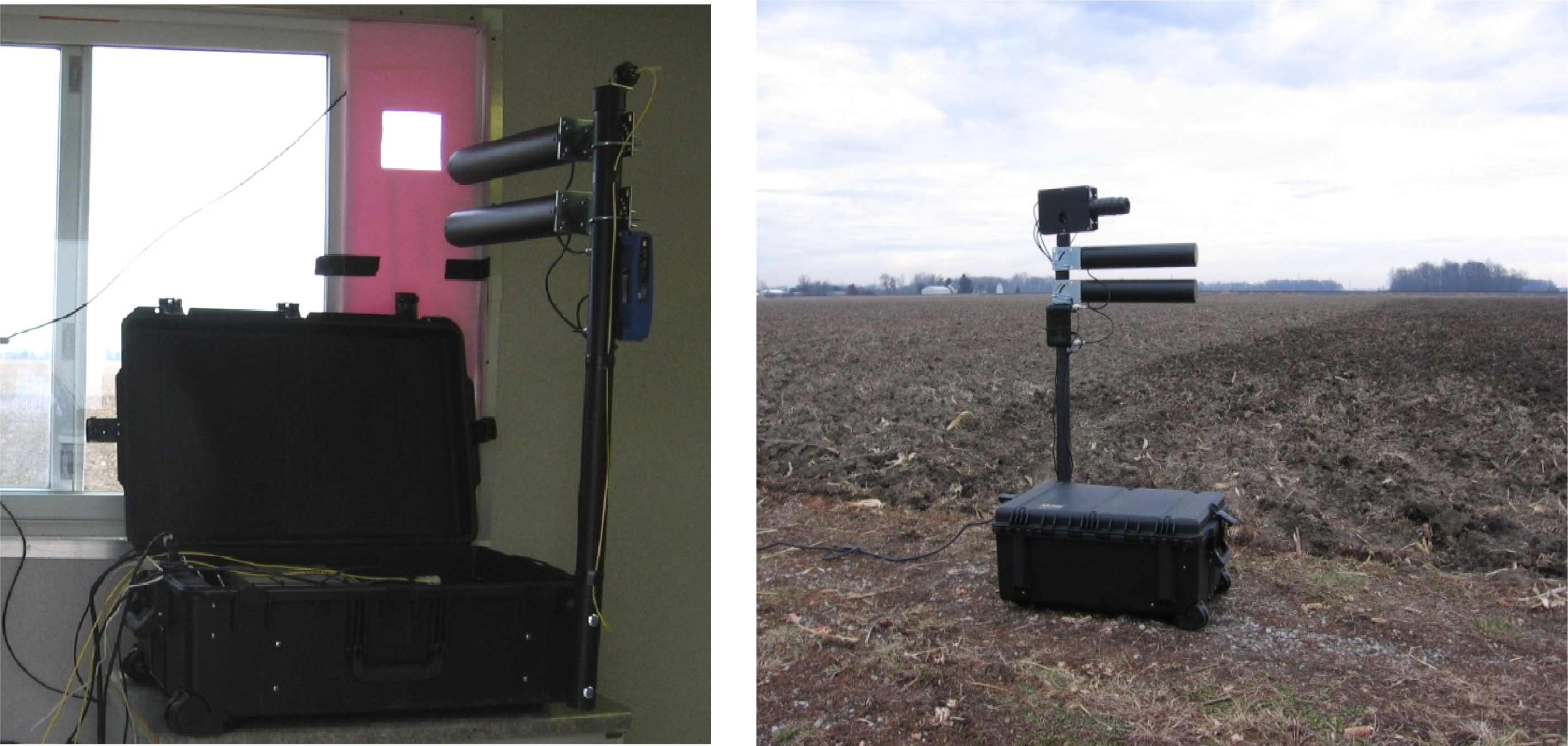
Both Tx/Rx, shown in
Figure 6, have a GPS receiver and Wi-Fi communication. The GPS receiver allows accurate time-stamping and precise geo-location. The Wi-Fi communication enables remote control and monitoring of the receiver functions from the transmitter location.
The LAnTeRN transmitter software was designed to control the laser wavelengths, the modulation intensity, and the modulation frequency while monitoring the wavelength of the online laser and controlling the relative intensity of the modulated laser signals. An algorithm was developed to actively maintain a fixed ratio of transmitted optical power between the two laser wavelengths in order to avoid introducing transmitter fluctuations into the received signal and to allow the receiver to operate without direct communication with the transmitter. In the case where the transmitter and receiver are co-located, the transmitter fluctuations can be divided out of the received signal using the transmitted beam as a reference. When the transmitter and receiver are separated, the software must maintain a fixed, known transmitted ratio of online to offline laser power. The latter case does introduce some noise in the system and limits the SNR that can be achieved. This limitation is discussed further in Section 3.
The receiver processor software utilizes a digital lock-in processing algorithm that allows for very long lock-in integration times. One challenge of long-integration lock-in processing is saving the high-sample-rate data for the duration of the lock-in period. The LAnTeRN receiver software overcomes this necessity with a near-real-time continuous lock-in algorithm that allows integration times of hours without using large blocks of memory. This capability, coupled with the stability of the frequency standards, allows the LAnTeRN system to make measurements at extremely low signal levels. The receiver software also provides a way to calibrate the system over a short transmission path to remove any frequency dependencies in the signal chain that would otherwise bias the measurement.
4. Experiments and Results
4.1. Laboratory Testing
Ongoing testing was performed throughout the entire system development process, starting in the laboratory and ending in the field. First, bench testing in the laboratory confirmed that the high-accuracy frequency standards could be used to synchronize the transmitter and receiver precisely enough to allow a high-precision measurement to be made with the transmitter and receiver operating remote from each other. This was done in an electrical loopback setup, where the transmitter electrical modulation signals were routed to the receiver analog-to-digital converter. With high-accuracy clock generators to synchronize the transmitter and receiver, the system proved to be time-stable at integration times of more than one hour.
The electrical loopback configuration was replaced with laser diodes, modulators, optics, and a detector and amplifier, using in-line fiber attenuators to reduce the transmitted power to the low levels expected in the field. In the absence of atmospheric interference, the system was able to achieve measurement SNRs of >1,000 at optical powers of tens of picoWatts and a lock-in averaging time of 60 s.
The next stage of testing used a gas cell and high-purity CO
2 gas to measure the accuracy of the LAnTeRN proof-of-concept system. Due to equipment limitations, we were unable to measure the cell pressure, and consequently, the expected differential transmission, to the level of accuracy desired, but we were able to show ratio measurement accuracy to within a few percent of the expected ratio. The 22 m gas cell was filled with 99.996% pure CO
2 gas at a variety of pressures ranging from 0 to 0.16 atmospheres. The combined-wavelength laser signal from the Tx was propagated through the cell and collected at the cell output by the Rx. Two pressure gauges were used to measure the CO
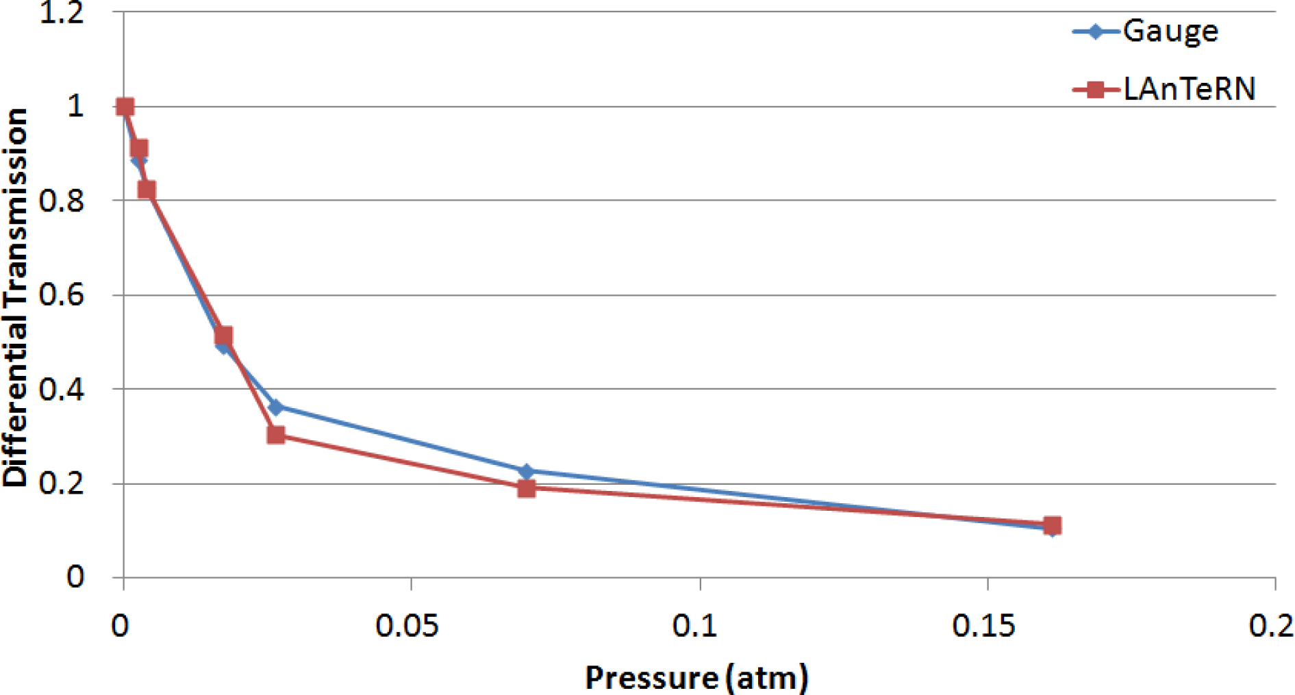
2 gas pressure—one at the cell and one at the pump. The pump gauge is most accurate at very low pressures, and the cell gauge is most accurate at higher pressures, so the theoretical (“truth”) ratios at intermediate pressures are the least accurate. The results of the gas cell test are shown in
Table 2 and
Figure 7.
The plots in
Figure 7 show the error at the intermediate pressures that can likely be attributed to errors in the gas cell pressure readings. The limitations of the pressure gauges can be overcome by using a scientific-grade gas mix with a CO
2 gas dry air mole fraction known to a very high precision. This gas can be used to fill the gas cell to near-atmospheric pressure where its pressure gauge is most accurate without complete absorption of the online laser signal. An alternative to gas cell validation is to take the system to a well-instrumented site with extensive
in situ measurements of the atmospheric state to validate against previously calibrated instrumentation.
4.2. Field Testing in Relevant Environment
The LAnTeRN proof-of-concept system was taken to Exelis’ outdoor test range, where it was set up and operated under a variety of conditions. The results of the field tests show that the system is measuring the differential transmission accurately to within about 0.5% relative to the model. The model used LBLRTM with a CO
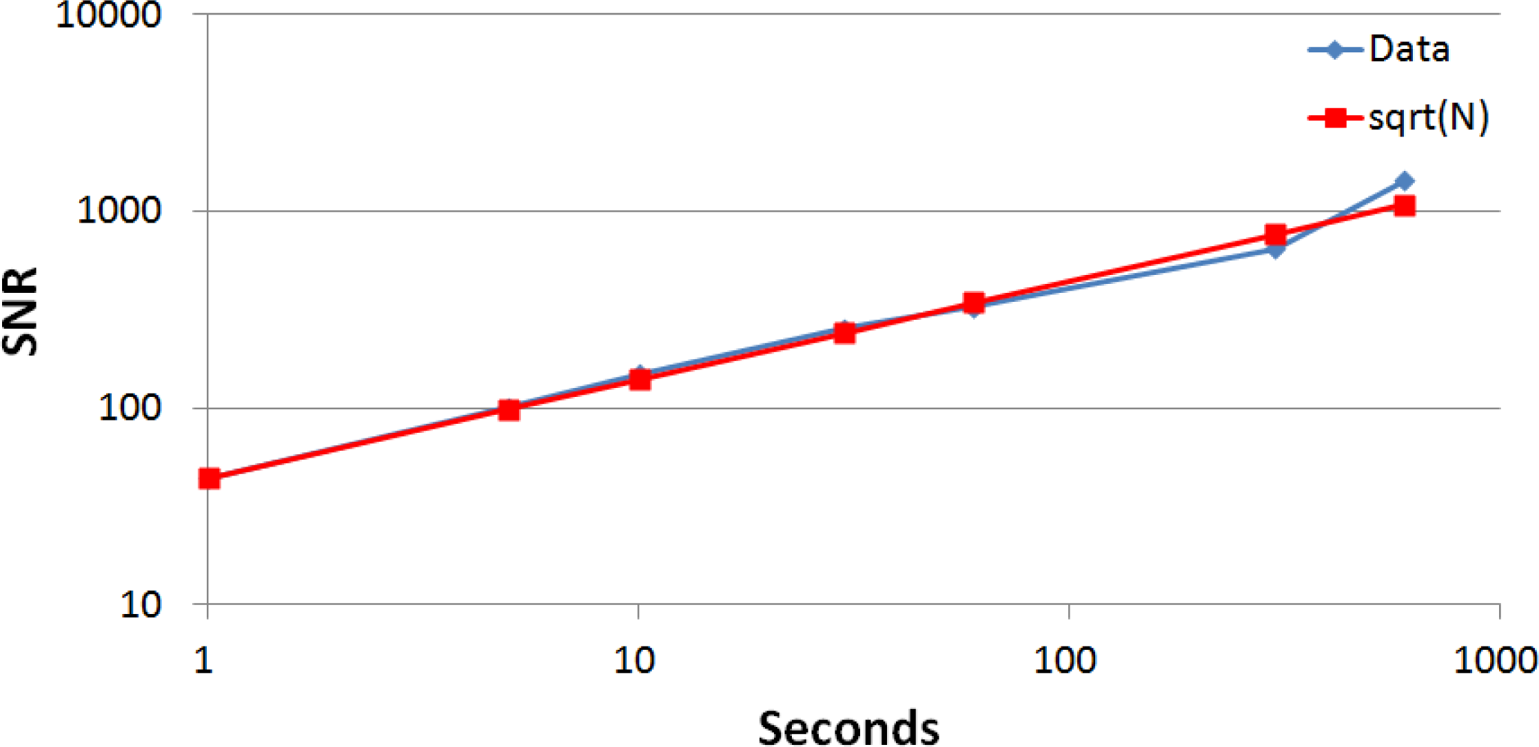
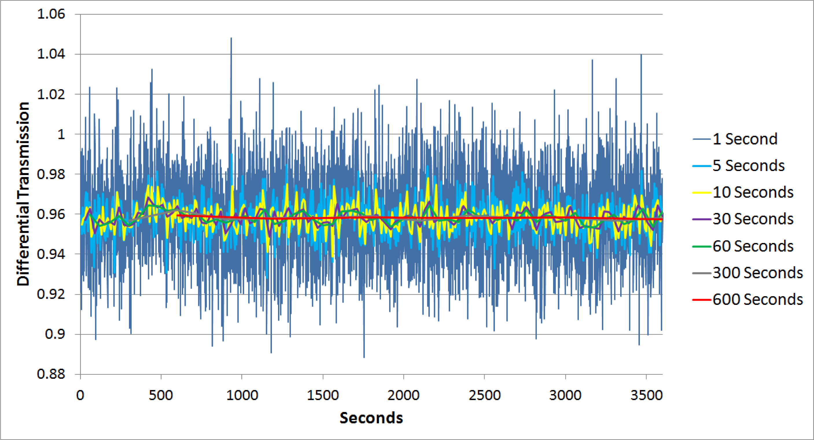
2 concentration of 380 ppm and the 1976 US standard atmosphere and temperature and pressure were taken from a local weather station. Until an absolute calibration can be performed, this level of performance verification is very good. The data also show the improvement in SNR that can be had by integrating (averaging) for longer periods of time.
Figure 8 shows that the averaging performance of the system closely matches the expected performance.
Figure 9 shows the ratio averaged at different integration times to show how significantly longer lock-in periods reduce the measurement noise. Note that the data used for
Figures 8 and
9 were taken early in the development and no calibration of the instrument was applied.
The field tests also show that the system is capable of performing near the theoretical limits.
Table 3 shows the instrument performance as compared to the physics-based performance model. The modeled and measured return power and differential atmospheric transmission are extremely close.
However, we believe the model under predicts the system SNR at low optical signal powers because it potentially underestimates the reduction of equivalent noise bandwidth resulting from the digital lock-in processing. This effect is not seen at higher return powers where atmospheric scintillation becomes the dominant noise term over the system electronic noise. Also note in the table that the model currently overestimates the SNR for the high signal and longer integration case. This is due to a limitation imposed by the transmitter’s ability to maintain a fixed ratio of the transmitted beams. The current system and algorithm are only able to maintain that ratio to about one part in 1,000, ultimately setting the maximum SNR that can be achieved through averaging.
5. Applications
The LAnTeRN concept could potentially be deployed in a number of space- and ground-based applications to provide high-fidelity measurements of column GHG dry air mole fractions. The most notable space-based application is the continuous monitoring of GHGs at a network of sites spread over an extended region, e.g., Eastern/Western continental US or Western Europe, with a single transmitter in geosynchronous orbit, possibly as a hosted payload on a communications satellite. A conceptual diagram of this configuration is illustrated in
Figure 10. In this configuration small ground-based receivers, placed within line-of-sight of a single stationary steerable or wide-angle transmitter located in geosynchronous orbit, would be able to collect data day and night, as well as through thin clouds and heavy aerosol layers. The portability of the ground receivers can enable focused studies in areas of key scientific interest such as mega-cities, boreal forests, or the tropics. Unlike the pulsed low-earth-orbit method proposed by Kuse
et al. [
32], this approach would allow a very robust validation campaign in order to determine and correct for bias, due to the continuous nature of the measurement. Initial calculations suggest that reasonable accuracies could be achieved with 8 W of average power from the transmitter and a 16 inch (406 mm) diameter telescope at the receiver and 2 minutes of integration at each receiver each hour. Due to this measurement concept being quasi-continuous, compared to a low-earth-orbit implementation, very high precision could be achieved through daily, weekly or monthly averages, and high accuracies could be obtained through extensive validation campaigns to determine bias. For a significantly lower cost than traditional space missions the LAnTeRN concept could be a key factor in monitoring, reporting, and verification for future policy, regulation, and treaties.
The LAnTeRN concept not only provides the potential for a novel, robust, low-cost approach for providing space-based measurements of GHG column dry air mole fractions (DAMF) at a number of fixed sites given a single transmitter located in geosynchronous orbit, it also can be used to provide a non-invasive method for autonomous and continuous monitoring of CO
2 and other trace gas DAMF and time-varying fluxes over an extended field site, such as a carbon sequestration facility, hydraulic gas fracking field, or volcano. The LAnTeRN approach could also provide a long-term technique for monitoring GHG distributions over an extended urban area. This is achieved by combining a limited number of transmitters with a network of receivers located around the perimeter of the desired area or a limited number of transmitter/receiver modules and reflectors distributed around the perimeter of the area with a field model to construct two-dimensional estimates of GHG distributions and time-varying fluxes. The latter concept is illustrated in the idealized field shown in the left-hand panel of
Figure 11. This figure shows a two-transmitter configuration with 58 receivers/reflectors located around an idealized 1 km × 1 km field. While the field illustrated in this example is highly regular in nature, the same concept can be applied to fields with irregular boundaries as long as an unobstructed line-of-sight exists between each transmitter and receiver/reflector pair. The figure also shows a representative set of synthetic plumes defined by a complex set of two-dimensional Gaussian distributions, and the red lines represent the possible transmitter/receiver measurement paths.
The resulting along-path measurements alone can provide an estimate of localized field DAMF and could be used to detect and estimate time-varying changes in local GHG DAMF. They also can be combined with a two-dimensional estimation technique to model the time-varying distribution of GHGs in the field itself. An example is shown in the right-hand panel of
Figure 11. This technique, which is based on prior work and has been demonstrated in a number of previous efforts using laser absorption spectroscopy and microwave attenuation to construct two-dimensional fields of CO
2 concentrations [
33] and rain rate [
34–
36] over defined areas of interest, models the field of interest as a limited set of base functions whose integrated intensities along the sampling paths best matches the observed values for a given set of best-fit criteria, e.g., mean-squared error. The resulting estimate from a prototype implementation of this approach is illustrated in the right-hand panel of
Figure 11. The fidelity of the resulting field distribution estimate and its location accuracy depends in part on how well the chosen analytical model matches the true field distribution, the placement of the transmitters and receivers, and the number of intersecting samples. While this approach is not designed to provide absolute measurements at discrete locations with sub-meter accuracy, it does capture the general shape and location of GHG plumes, which are normally diffuse in nature, and provides a robust method for tracking time-varying aspects of their distributions.
The reflector configuration depicted reduces the cost of this type of mapping operation and is well suited for some applications like carbon sequestration sites, but would be impacted by large aerosol concentrations in applications like volcano monitoring, due to partial path returns. However, several similar implementations are possible, for example using transmitter/receiver pairs in all four corners can enable direct transmission measurements over several transects in order to determine and correct for potential bias from intermediate scatter sources under those circumstances.
6. Conclusions
We have briefly described the theory, development, and demonstration of a new prototype instrument for measuring GHGs in the atmosphere. Several advantages over exiting methods for both ground-to-ground and space-to-ground have also been discussed. The LAnTeRN prototype instrument successfully demonstrated the potential for this open-path LAS measurement concept to provide high precision measurements over long path lengths, and at very low received power levels. The prototype measurements also served to validate a high-fidelity physics-based performance model that can be used to optimize future developments for specific applications. Further testing is planned for a detailed evaluation of instrument precision and accuracy. Other further developments will include locking rather than measuring the transmitter wavelengths, as would be required for a space-based approach, and building a more complete model by including other noise sources such as the laser stability and intensity fluctuations.
The instrument has a wide range of potential applications, which were only briefly touched on here. The range of applications spans ground-to-ground and space-to-ground implementations. The measurement capability compliments current ground-based in situ instrumentation by providing an integrated path measurement, both day and night, that is not biased by heavy aerosol concentrations in the path, and can be implemented to provide concentration and time-varying flux maps over a large area. Furthermore, the space-to-ground application complements current and planned space monitoring of GHGs by adding high spatial and temporal resolution measurement capability which, through averaging and the ability to evaluate and determine bias, will enable measurements to the precisions and accuracies required to distinguish anthropogenic and biogenic sources and sinks. The authors look forward to discussing further developments towards these and other applications in future publications.


