Airborne Thermal Data Identifies Groundwater Discharge at the North-Western Coast of the Dead Sea

Abstract

A qualitative and quantitative monitoring of groundwater discharge was conducted based on an airborne thermal campaign undertaken along the north-western coast of the Dead Sea in January 2011 to contribute to the relatively scarce information on groundwater discharge to date in the region. The application of airborne thermal data exploits thermal contrasts that exist between discharging groundwater and background sea surface temperatures of the Dead Sea. Using these contrasts, 72 discharge sites were identified from which only 42 were known from previous in situ measurements undertaken at terrestrial springs by the Israel Hydrological Service. Six of these sites represent submarine springs and at a further 24 locations groundwater appears to seep through the sediment. Although the abundance of groundwater seepage sites suggests a significant, but so far unknown groundwater source, the main contribution appears to originate from terrestrial springs. In an attempt to provide a quantitative approach for terrestrial springs, a linear bootstrap regression model between in situ spring discharge and respective thermal discharge plumes (r² = 0.87 p < 0.001) is developed and presented here. While the results appear promising and could potentially be applied to derive discharge values at unmonitored sites, several influence factors need to be clarified before a robust and reliable model to efficiently derive a complete quantitative picture of groundwater discharge can be proposed.

1. Introduction

The surrounding area of the Dead Sea (DS) is heavily reliant on groundwater as major water resource for domestic and agricultural water supply [1]. Some authors even state that current groundwater abstraction exceeds available resources which would imply overexploitation [1,2], thus requiring sustainable groundwater management to establish and secure water availability for future generations. In this context, knowledge of uncontrolled groundwater loss is essential for future water management strategies [3]. However, existing groundwater discharge estimates for the western DS coast are discrepant varying between 30 and 96 × 10⁶ m³·a⁻¹ [4–6].

In the interest of obtaining more accurate discharge volumes the Israel Hydrological Service (IHS) initiated a monitoring program in 2004 [7]. Within the program groundwater discharge is measured biannually at terrestrial springs of the main spring areas of Ein Feshkha, Kane and Samar. These springs are favorable discharge measurement locations since they allow a quantitative assessment of the discharge of large catchments at individual and well defined locations (e.g., intersecting fault zones). It is assumed that at these intersections groundwater emerges and discharges via erosion channels into the DS. The continuous discharge measurement in turn reveals important insights into groundwater flow dynamics. However, IHS measurements are limited and cover ca. 50% of the western DS coast and do not yet account for discharge from submarine springs [8]. Although increasingly observed, their contribution has not been determined to date mainly due to the appreciable challenge in measuring submarine groundwater discharges directly. Moreover, the total abundance and the precise locations are as yet unknown. This information is critical to the development of sustainable water management planning initiatives.

To provide information on unknown submarine spring locations and to test whether an alternative groundwater discharge mapping/monitoring approach provides comparable results to in situ observations we pursued an airborne thermal campaign in January 2011 spanning the northwestern part of DS coast (Ein Feshkha) where both terrestrial and submarine springs are found. Recent research has shown that thermal data has the potential to be used to gain information on groundwater discharges across large spatial scales. Such information for example might include the localization of submarine groundwater discharge [9–13] and the respective quantification [14–16]. Moreover, it is possible to infer groundwater discharge amounts based on a linear [16] or logarithmic [14] regression analysis between the thermal plume area induced by discharge and in situ measured discharge volumes.

Based on the obtained airborne thermal data the first objective of the present study is to identify all groundwater discharge locations within the study area, particularly with submarine origin and subsequently to provide a spring discharge inventory. The results are compared to in situ IHS data discussing the applicability of airborne thermal data to provide a complete qualitative picture of discharge locations. The second objective is to test the feasibility of deriving discharge rates from single springs based solely on thermal data. As the positive result would provide an effective quantitative discharge monitoring option over large spatial scales, it is likewise of interest to discuss advantages and limitations that might arise in parallel. Both objectives potentially set the foundation for an efficient qualitative and quantitative discharge monitoring and for a future implementation of a sustainable groundwater management plan of the western catchment of the DS.

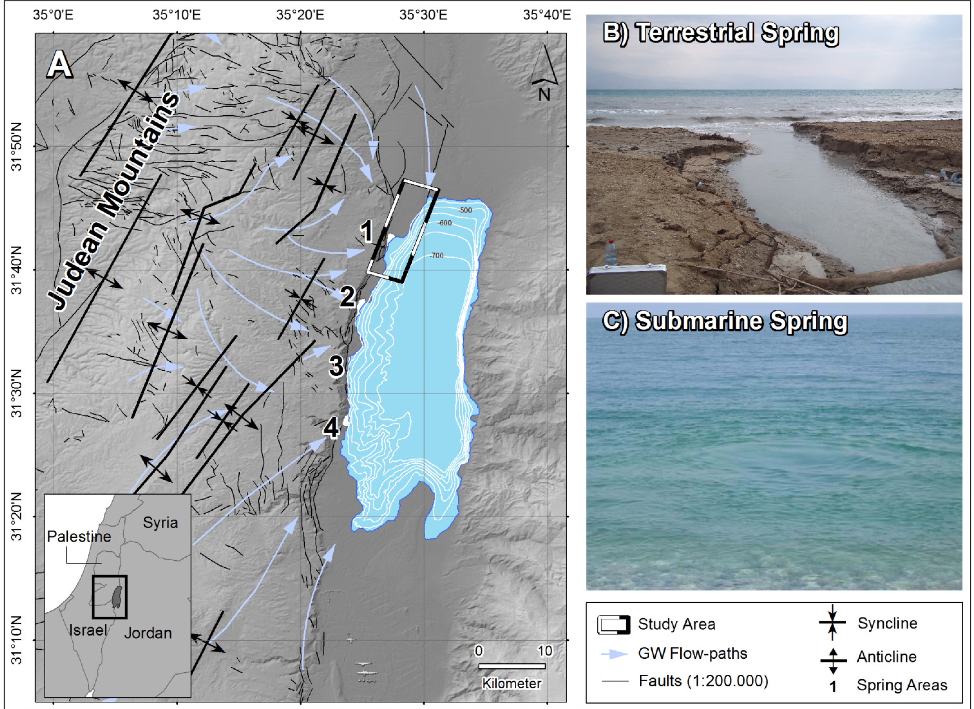
2. Study Area

The DS is a terminal lake situated in the Jordan Dead Sea Graben surrounded by 300–500 m high escarpments formed by normal faults [17]. Ein Feshkha is the largest known spring area located at the northwestern part of the DS. Emerging groundwater at this site originates from two main aquifers. The first, the Judea Group Aquifer, is comprised of limestone and dolomite rocks from upper and lower Cretaceous ages that is divided into an upper and lower sub-aquifer. It is replenished mainly in the region of the Judean Mountains that reflects the outcrop of this aquifer and likewise the region of highest precipitation (400–600 mm·a⁻¹) [18]. The second aquifer, the Coastal Alluvial Aquifer developed during Quaternary age within the Jordan-DS Graben and is composed of aragonite, gypsum and clay varve sediments. At outlets of intermittent streams (wadis), this main type of background facies is intercalated with gravel, sand and pebble deposits [17]. Groundwater within this aquifer is replenished through the Judea Group Aquifer and possesses a negligible replenishment from precipitation that amounts to ∼50 mm·a⁻¹.

Faults and folds with mainly E-W and SW-NE orientations control the general groundwater flow in the Cretaceous aquifers. Within the coastal alluvial aquifer the general flow-direction partly changes as Holocene structural features have ESE-WNW orientations with extensional directions of NNE-SSW [19]. Due to the structural control groundwater emerges at distinct locations. Several authors describe the spring areas of Ein Feshkha, Kane/Samar, Qedem and Ein Gedi (Figure 1A) [4,18]. These areas are mainly characterized by aforementioned terrestrial springs that subsequently form erosion channels due to the lowering of the DS with currently 1.0–1.3 m per year (Figure 1B). The second spring type, submarine springs, emerge at the sea bottom down to a depth of 30 m [8]. Density differences between groundwater (1.00–1.19 g·cm⁻³) and DS water (1.234 g·cm⁻³) trigger a continuous density driven upward buoyancy flow of the emerging groundwater (see

Table 1. Hydrochemical values between groundwater along the Dead Sea and Dead Sea water.

Parameter	Dead Sea	Groundwater	Source
Temperature (°C)	22–33	25–30/41–44 *	Hact & Gertman [20]
Density (g·cm−3)	1.234	1.00–1.19	Own measurements
TDS (g·L−1)	345	1–35/184–204 *	Own measurements
Salinity	300–338	0.82–88.4	Ionescu et al. [8]

^*Value ranges for thermal water of Qedem springs.

[8,20] for typical hydrochemical groundwater and Dead Sea water values). When rising groundwater approaches the sea surface it can become visible as a circular upwelling pattern [17] (Figure 1C [21]).

Typical groundwater temperatures of both aquifers are 26–28 °C [22,23]. Own measured temperatures at the springs display yearly constant values ranging from ∼25 to 29 °C (Ein Feshkha), to ∼25–30 °C (Kane), to ∼28–30 °C (Ein Gedi), to ∼41–44 °C (Qedem) independent of spring type (note that most Qedem springs are associated to the deeper Kurnub aquifer that is not described in this study). In contrast, the DS surface temperature follows the yearly air temperature. This produces long-term minimum temperatures of ∼22 °C between December and March and long-term maximum temperatures of ∼33 °C between July and September, respectively [20]. The temporal change of DS water temperature induces a contrast with maximum values of >3 °C in high winter and summer periods to aforementioned groundwater temperatures that remain nearly constant over time. In turn, groundwater discharge can be identified exploiting the thermal contrast, as pursued in the current study.

3. Data and Methods

3.1. Airborne Campaign

The airborne thermal campaign was conducted in January 2011. Although the entire western DS coast was covered during 4 night flights (11/13/16/18 January) between 2 and 5 a.m. local time we present here only the first area at the north-western part of the Dead Sea (Ein Feshkha) recorded on 11 January. Flight altitude over the sea surface was at 1,000 m above ground (575 m a.s.l.) providing data with a ground sampling distance (GSD) of 0.5 m. To ensure optimal coverage the overlap between the single data was >30%. Additionally we pursued an aerial survey on 22 January between 10 h and 14 h local time to complement the thermal campaign. The GSD for the aerial photographs is also 0.5 m and the overlap was >50% to allow an appropriate subsequent stereoscopic analysis.

The used AERO-FE sensor system from the German Federal Institute for Geosciences and Natural Resources was mounted on a Piper Chieftain Navajo PA31 aircraft and comprises:

• A thermal camera Infratec VarioCam hr head with an uncooled microbolometer as radiation (temperature) detector and a focal plane array of 640 × 480 pixel
• An aerial RGB camera Rolleimetric AIC P25
• Three axis gyro-stabilized platform AeroStab-2 to maintain nadir view of the mounted sensor
• A GPS/IMU to continuously log aircraft position and rotation
• Flight management system AeroTopol

The thermal sensor spans the 7.5–14 μm fraction of the electromagnetic spectrum and possesses a temperature resolution of 0.08 K. The recorded radiation is converted into a 16 bit format to maintain the high-resolution temperature differences.

Ground truth measurements conducted to support the aerial and thermal surveys were homogeneously distributed over the entire investigation area. These encompass the (i) dGPS information to geo-reference the airborne data, (ii) land and water temperatures to compare and possibly adjust atmospherically corrected thermal data and (iii) in situ discharge volumes of terrestrial springs as a basis for the discharge volume/thermal plume relationship (

Table 2. Type and number of conducted ground-truth measurements for position, reference temperatures and spring discharge volume—Note that the water depth of Onset HOBO^® TidbiT Temploggers was ∼3 cm.

Ground-Truth	Location	Device	Number of Reference Measurements
			Total	Study Site
Position	Land	Trimble GeoExplorer XT	33	6
Temperature	Land	Ahlborne AMIR 7814-20 Remote Thermometer	50	14
	Water	WTW 340i (discrete measurements)	36	2
	Water	Onset HOBO® TidbiT v2 Templogger (continuous measurements)	12	2
Discharge volume	Water	Flo-Mate™	40	4

).

Recorded aerial photographs were geo-referenced and orthorectified supplemented by the dGPS ground-truth measurements through a bundle block adjustment. The resulting absolute horizontal (vertical) accuracy amounts to ∼0.5 m (∼1.0 m).

Thermal data are converted from recorded radiance data to surface temperatures by inverting Planck’s law (Equation (1)). The equation considers an inverse function of the sensor-specific temperature curve between 7.5 and 14 μm, an emissivity value of 0.97 (water at salt concentrations >34‰) and the radiance of a given mean air temperature at the time of recording:

$${\vartheta }_{\mathit{surf}}=\left[{\Phi }^{-1}\left(\frac{{\Phi }_M-(1-\epsilon )\cdot {\vartheta }_{\mathit{AT}}}{\epsilon }\right)\right]-273.15$$

(1)

where ϑ_surf = surface temperature (°C), Φ⁻¹ = inverse function of the sensor-specific temperature curve (1/W·cm⁻²), Φ_M = measured surface radiation (W·cm⁻²), ε = emissivity (−), ϑ_AT = ambient air temperature (°C).

Before the so calculated surface temperature data set obtained through the aerial surveys could be compared to ground-truth data, a malfunction of the thermal sensor system meant that the geo-referencing had to be completed manually. This was conducted by identifying distinct patterns in each surface temperature image that were subsequently defined as tie points for mosaicking all images to a complete data set. The complete data set was afterwards co-registered to generated orthophotos using a 2nd order polynomial transformation with an accuracy of ∼1.5 m (three pixels).

3.2. Discharge Measurements

For the presented study area only four in situ reference measurements on spring discharge are available. To obtain a larger reference data set and hence less uncertainty for further analysis we revert to the IHS spring discharge data set [24] that contains 44 measurement locations in the study area. This however requires a prior descriptive and statistical comparison between both discharge data sets as they differ in time (two months) and processor that may result in measurement bias.

The IHS method to obtain spring discharge volumes corresponds to the method applied here. This includes (i) pursuing measurements at a homogenous and straight flow section, (ii) recording a detailed channel cross-section and (iii) obtaining likewise detailed flow velocity fields. To account for the latter two, measurements were well distributed at vertical and horizontal spacings of 10–20 cm at which velocities were obtained through an electromagnetic current meter (Flo-Mate™—Table 1) [25]. The only difference between IHS and own measurements concerns the time of recording. While our measurements were conducted on 14 January 2011, IHS measurements were recorded on 17 March 2011. Results of the statistical comparison between both discharge data sets are discussed in the Results and Discussion section.

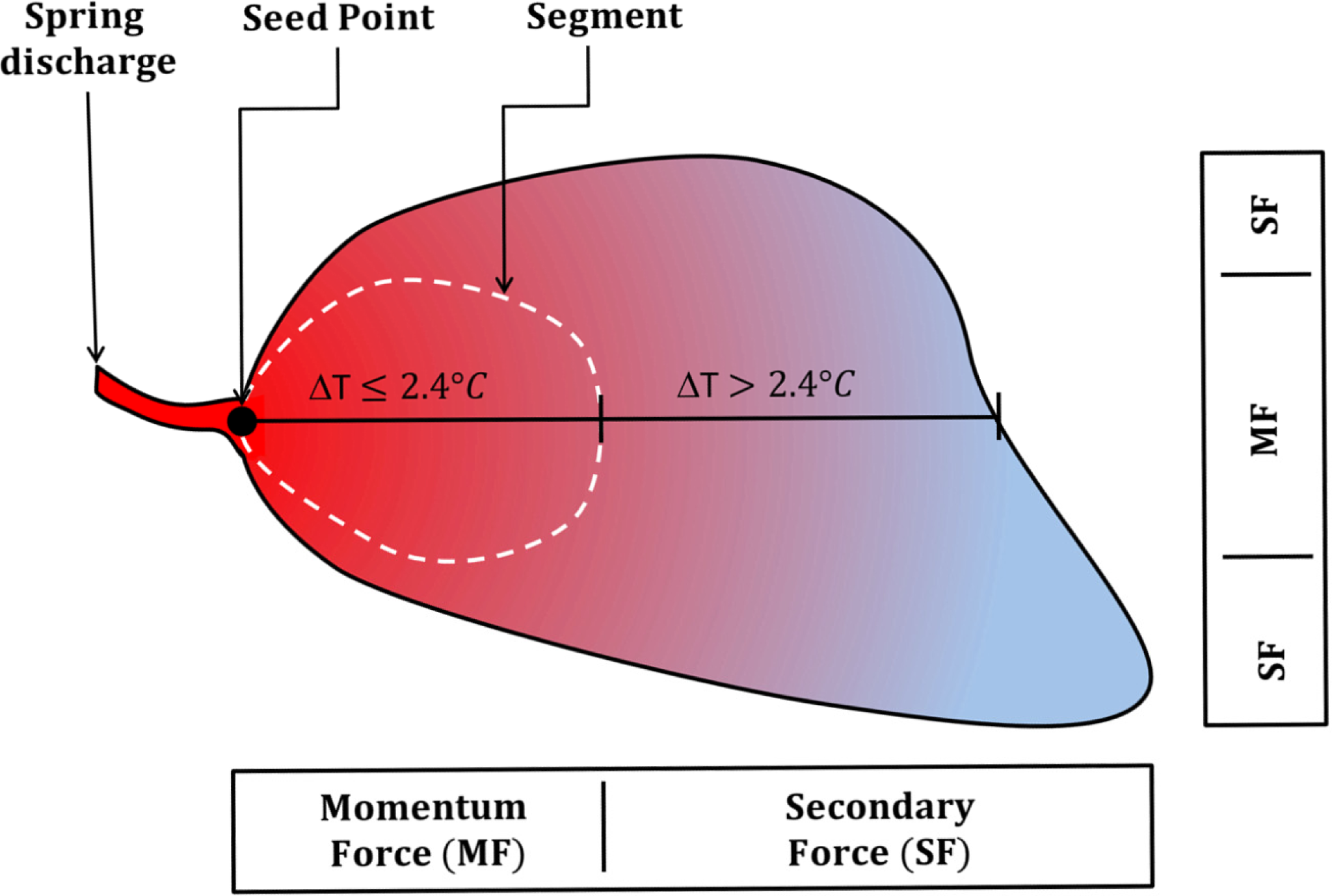
3.3. Segmentation Approach for Discharge Quantification of Terrestrial Springs

Differences in water temperature between discharging groundwater and open water bodies result in the development of a thermal discharge plume that can be traced through sea surface temperatures contrasts. Under the simplified assumption that observed sea surface temperature adapts uniformly in a radial manner off the spring outlet we suppose a linear relationship between spring discharge volume and temperature adaption that is expressed as temperature decrease for the present study. This assumption is most likely true as long as the governing force is the spring discharge momentum (product of discharge velocity and volume). Findings of Roseen [16] and Danielescu et al. [14] support this assumption who found a uniform linear relationship between cumulative plume area and surface temperature until a maximum temperature change of ∼5 °C. As this number is most likely depending on local conditions, we focus on small temperature changes only for which we assume discharge momentum to be the governing force. Large temperature changes could be affected by secondary forces such as wind or currents that individually change temperature distribution and would consequentially lead to erroneous results.

Following this assumption we apply a region growing approach [26] to extract comparable areas with small temperature changes. This approach groups all pixels into segments that fall within a given threshold emanating from a seed point (Figure 2). Since it is of interest to extract the thermal plume area off a discharging spring we defined the outlet as seed point. From the reference temperature at this seed point we applied a user defined threshold of 2.4 °C. This threshold (i) orientates on local conditions (total temperature contrast, secondary forces, etc.); (ii) considers aforementioned findings of Danielescu et al. [14]; (iii) reflects momentum force governed areas only and (iv) was rounded to 2.4 °C in order to account for the camera temperature resolution of 0.08 °C (results in factor 30 and the threshold of 2.4 °C), i.e., all pixel that maximal differ by this threshold value are segmented (grouped). The threshold value was repeatedly used at 16 spring discharge outlets from which the discharge volume was known from IHS measurements. In cases where several springs emerge in a close-by environment and merge into one thermal discharge plume, we subsequently related the thermal plume area to the accumulated discharge volume. The described procedure assures a comparability between different thermal plume areas accounting for the fact that spring water varies in temperature between ∼25–29 °C.

4. Results and Discussion

4.1. Comparison between Measured and Modeled Surface Temperatures

The resulting ϑ_surf from Equation (1) was compared to in situ measured surface temperatures. As Figure 3 shows surface temperature values deviate from the 1:1 line particularly for cooler land temperatures. However, a certain trend can also be observed that is described by a linear regression in the form of Equation (2):

$${\vartheta }_{\mathit{surf}}=0.68x+7.30$$

(2)

The resulting r² = 0.90 and significance value of p < 0.001 underlines the relationship and allows to obtain real surface temperature values by applying Equation (2) to the surface temperatures resulting from Equation (1). The consequential real surface temperature values overestimate land temperatures but water temperatures, that are relevant for the present study, are well depicted emphasized by the good correspondence to in situ measured water temperatures.

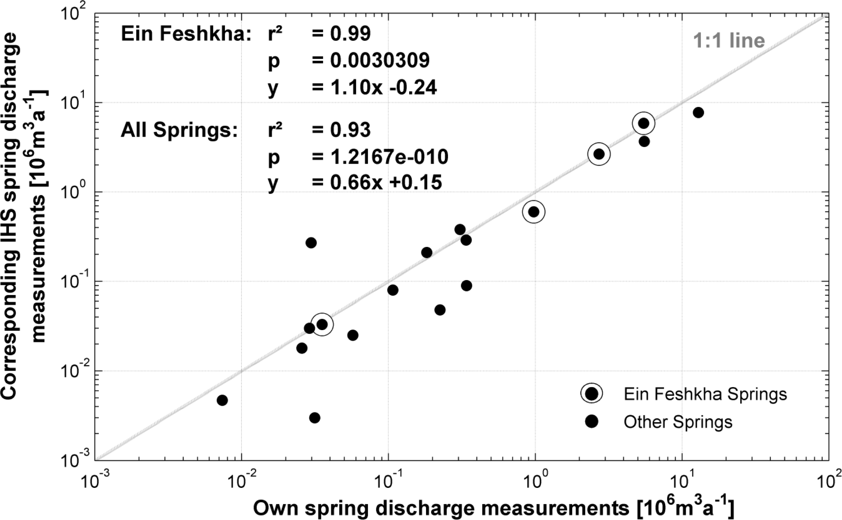
4.2. Comparison between Own and IHS in situ Measured Spring Discharge

The comparison between own and IHS in situ measured discharge values of all corresponding locations (Figure 4) along the entire western coast reveals a small scatter along the 1:1 line and a satisfying agreement (r² = 0.93, p < 0.001). In particular the IHS measurement for the Ein Feshkha springs deviate only slightly from the 1:1 line with a maximum difference of 0.4 × 10⁶ m³·a⁻¹ only. This fact underlines that spring discharge volumes display almost no differences despite the time difference of two months between the recording of own and IHS obtained discharge measurements. This time independency is also shown in the study of Vachtman and Laronne [27] who report for the same area a temporal discharge stability over two years with almost no variability. Hence, due to the number of measured springs located in the thermally covered area and the temporal discharge stability the IHS data set is more appropriate for further analysis. Own in situ discharge measurements were discarded for the following analyses.

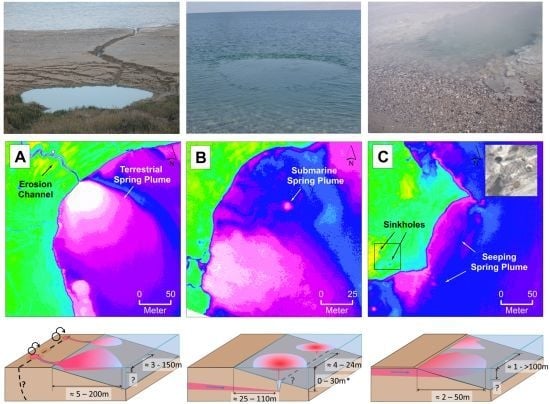
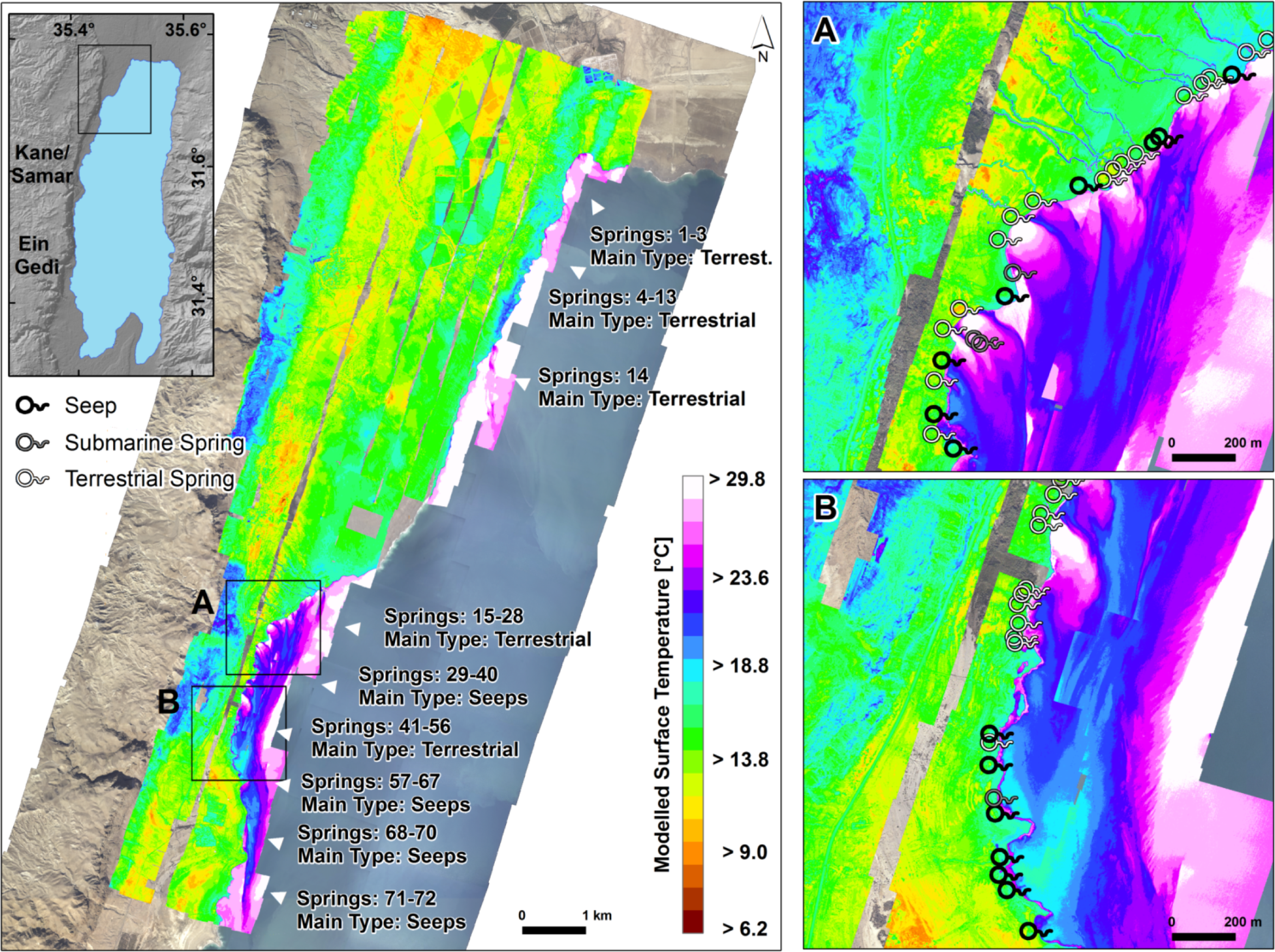
4.3. Identification of Groundwater Discharge Sites

The high-resolution airborne thermal data (Figure 5) range in general from 6.2 °C to 34.3 °C (note that these temperatures are obtained through Equation (2)). Terrestrial areas possess temperatures below 13 °C except for steep sections of the cliff at which the apparent temperature is ∼20 °C. Water on the other side possesses clearly distinguishable temperatures. Discharging groundwater displays values of ∼23–28 °C. Depending on the momentum force of the discharge, a lateral thermal plume with varying size develops, in which the sea surface temperature gradually decreases towards the center of the Dead Sea. After a certain distance the inflowing water is deflected southwards through a secondary force that most likely can be attributed to a local current. At this deflection point sea surface temperatures are lowest with ∼19 °C. Similar low values exist at the southern end of the study site and in between thermal plumes of adjacent springs. Towards the center of the DS sea surface temperatures appear to increase again to slightly lower values (∼27 °C) than discharging groundwater.

These temperature contrasts allow outlining 72 groundwater discharge sites. The main clusters are indicated by white triangles in Figure 5 (note that all discharge sites are listed in Appendix Table A1). We classified these sites according to the known spring types in terrestrial and submarine springs depending on the location, the presence of an erosion channel and typical thermal plume shapes (Figure 6).

The classification identifies 42 groundwater discharge sites with terrestrial origin mostly located along concave or straight coastlines. Taking the entire discharge site abundance for the study area as reference it is most likely that terrestrial springs are the main contributor of groundwater to the Dead Sea. Their thermal plume extents vary in shape, with plume lengths along the central axes ranging from ∼5 to 200 m (Figure 6A). 40 thermally identified springs spatially match 44 IHS approved discharge sites of the same area and two identify so far unmonitored sites [24]. The discrepancy of four springs between thermally identified terrestrial springs to 44 IHS sites concern springs with a discharge volume of less than 0.008 × 10⁶ m³·a⁻¹. Their accumulated amount that could not be clearly identified by the airborne thermal data, results in a negligible share of 0.04% given the IHS measured total groundwater discharge of 59.0 × 10⁶ m³·a⁻¹.

Apart from the terrestrial springs, the thermal data reveal six spring locations of submarine origin. One of these submarine springs and the resulting circular thermal plume shape is shown in Figure 6B. These springs vary in thermal plume diameter between ca. 4 and 24 m and are located at a distance between 25 and ca. 110 m to the shoreline. Available bathymetric data is too imprecise to deduce exact emergence depths of each spring but given the mentioned distances to the shoreline and the low-inclined sea floor suggests emergence depths to be most likely in the same range (<30 m) as Ionescu et al. [8] report.

At four locations we identify single circular plumes and no clustering. Two further submarine spring sites form clusters with two or more springs whose spacing between single springs is 20–25 m. The clustering again corresponds to findings of Ionescu et al. [8] who report the same characteristics along the nearby region north of Wadi Darga. Single springs within submarine spring clusters (indicated by a dashed line in the schematic view of Figure 6B) even appear to be arranged in a shore parallel and linear manner with orientations of ∼350° and 60°, respectively.

Based on the currently available thermal data groundwater contribution from submarine springs for the investigated area (Ein Feshkha only) appears to be <10% considering the total spring abundance (n = 72) as reference. It is most likely that this number represents only a minimum as (i) the thermal signature from the terrestrial springs may camouflage the thermal signal from near-shore submarine springs at the same location and (ii) water of submarine springs with minor discharge and a emergence in larger depths exhibit a less clearer thermal signal on the sea surface or cannot be traced as it could get completely mixed before reaching the sea surface.

A third spring type can be identified at 24 locations not yet described in the literature to occur at the Dead Sea coast. This spring type is located adjacent to mostly exposed, convex or straight shorelines. The thermal plumes range between 2 and 50 m in length perpendicular to the shoreline, while their extents parallel to the coast stretch between a few tens to several hundreds of meters (Figure 6C). These types of springs/seeps are neither accompanied by an erosion channel nor do they display a circular thermal plume. This is the reason why they cannot be attributed to the type one and type two spring types.

The abundance of groundwater with a considerable lateral flux at these locations is given as water filled sinkholes exist nearby that are caused through salt dissolution by passing groundwater under-saturated in respect to halite [28,29]. The thermal data suggest theses springs to discharge diffusely at the land/water interface either on land or submarine over large (>100 m) coast-strips, which is backed by in situ observations (Figures 6C and 7A). At other locations this spring type also occurs rather locally over coast-strips <100 m (Figure 7B). At one location we find an outstanding thermal plume similar to plumes from terrestrial springs but no erosion channel which suggests an emergence at the land/water interface such as a seeping spring (Figure 7C). Discharge at this location comprises a concentrated inflow with a presumably high volume over a distance of ∼100 m possibly formed by several adjacent single springs. However, the high and concentrated discharge that moreover appears to have caused a landslide lets us presume that governing processes for this discharge are rather similar to terrestrial springs. These will probably lead to the evolution of this spring towards a non-ambiguous terrestrial spring within the following years. As this is the only location with such a constellation, it most likely represents an exception.

The prevailing lacustrine sediment composition is fine-grained comprising different colored varves with variable content ratios of clay, aragonite and gypsum. This fine-grained and compact sediment with a low primary hydraulic conductivity lets groundwater most likely discharge diffusively over large continuous coastal strips (Figure 7A,B). At certain locations (as shown in Figure 7C) groundwater might possibly concentrate in form of e.g., preferential flow-paths (secondary porosity) with high conductivities along Holocene faults or folds [20] to subsequently emerge at distinct points.

A further explanation for seeps could be the flushing effect that Kiro et al. [30] and Yechieli et al. [31] describe. The rapid drop of the Dead Sea level, which enforces the hydraulic gradient between the aquifer potential and the lake level, explains this effect. Since the system is assumed to be in equilibrium, the rapid drop leads to an increased ground- and porewater discharge (flushing) until the new dynamic equilibrium is reached [30]. This mechanism is likely to be valid along larger sections of the coastline rather than distinct points and hence is likely the origin of the continuously seeping springs.

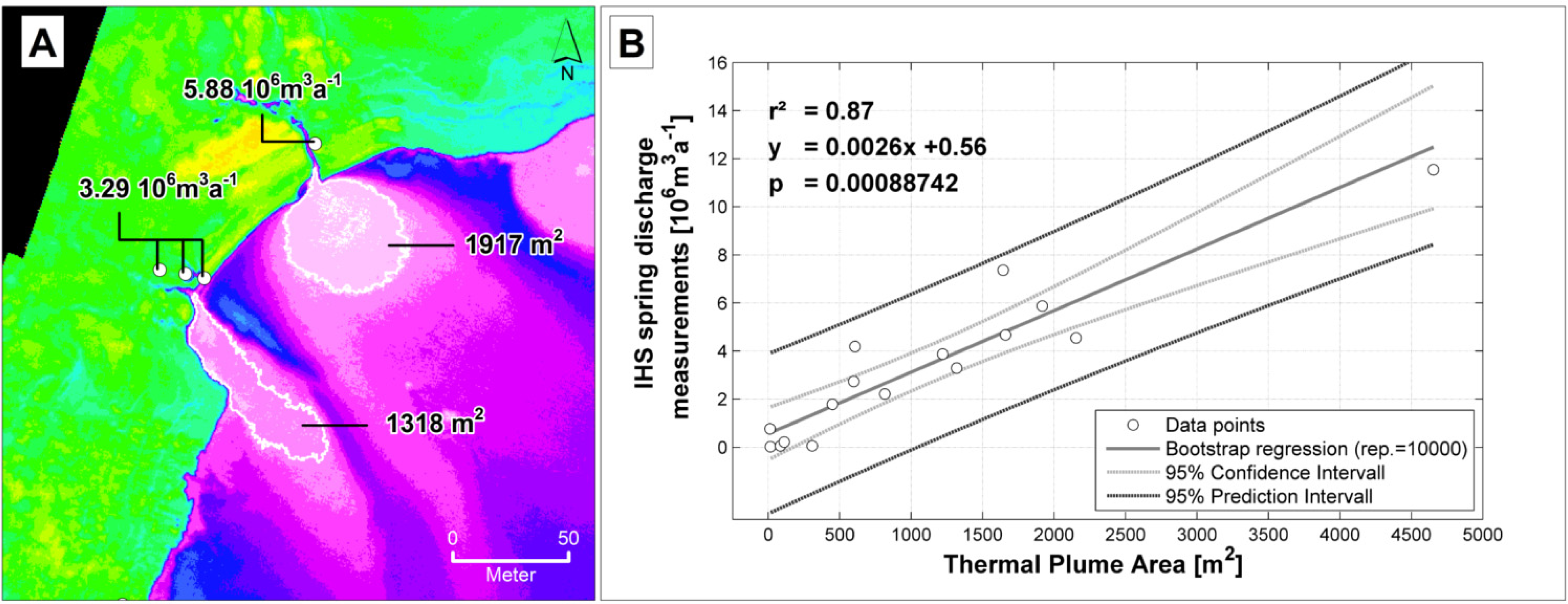
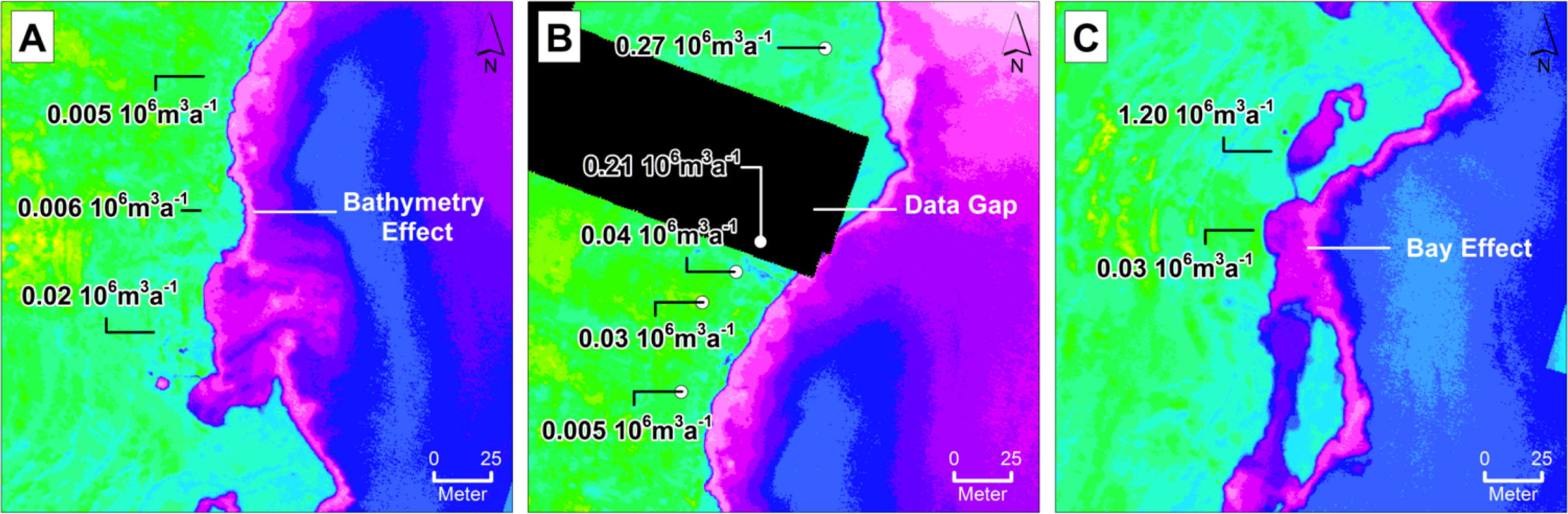
4.4. Attempt to Quantify Groundwater Discharge

Figure 8A shows the result of the segmentation with corresponding areas at two discharge site examples. Plotting the so derived segmented thermal plume areas of all 16 sites against the according measured discharge volumes reveals the expected linear relationship (Figure 8B). The coefficient of determination (r²) from the linear bootstrap regression amounts to 0.87 with a significance of p < 0.001 underlining the significance of the relationship between both parameters and proving our segmentation approach. The modeled discharge volume with the bootstrap regression amounts to 54.9 × 10⁶ m³·a⁻¹ and hence, explains 93% of the total IHS measured volume of 59.0 × 10⁶ m³·a⁻¹. Yet, despite the thoroughly strong correlation, the corresponding significance and the conformity of the linear relationship to findings described by Danielescu et al. [14] and Roseen [16], we still consider the quantification approach as an attempt. Several factors exist that possibly influence the quantification result.

The exponential adaption of water temperatures as it drains into the cooler Dead Sea water leads to a faster temperature adaption for spring water temperatures with higher ΔT in respect to the Dead Sea temperature compared to spring water temperatures with smaller ΔT values [32]. This in turn might affect the comparability between segmented thermal plume areas of differently tempered spring water and hence the modeled discharge quantity. Since our thermal result shows a rather uniform distribution of spring SSTs at the seed points of 29.0 ± 1.4 °C we expect no significant effect on the segmentation result.

A second influence could derive from non-uniform occurring turbulences and the subsequent differences in mixing of water/temperature. This cause addresses varying discharge velocities (note that own measurements differs between <0.1–1.30 m·s⁻¹), an undulating sea floor or higher wind velocities. At the time of the campaign the latter was 4.0 ± 0.5 m·s⁻¹ and therefore slightly above the monthly median of 3.4 m·s⁻¹ (wind data are recorded at Ein Gedi coast station by the Israel Oceanographic & Limnological Research). In contrast to aforementioned influence factors, wind (direction and velocity) will not significantly affect the thermal plume development and hence the segmentation result, if we consider a small time span in between recording as given for the presented campaign (3 h). Comparing different days however might significantly influence the result induced by varying conditions.

Regarding the influence of varying velocities, it is conceivable that larger springs with higher velocities might adapt differently than smaller springs that again could influence the segmentation and modeling results. In this context it is furthermore unclear how the sediment load affects the heat transfer. Higher spring discharge could carry an increased sediment load that most likely possesses a slightly different heat capacity than slow spring discharge with no suspension load. Since turbidity of spring water was not investigated, the differing heat capacity and hence a varying heat transfer between spring water and the Dead Sea cannot be excluded as potential third influence.

A fourth influence could also arise through convective heat transfer from the sea bed. We partly observe such an effect along the DS coast. However, the influence strongly depends on the local bathymetry. While shallow areas most likely exhibit an influence, a steep and likewise deeper bathymetry possesses almost no influence. According to observations of Ionescu et al. [8], a steep decline of the sea bed is observable at a distance from the shore of about 5 m. This results in a near-coast effect (Figure 7B) with a “heated” fringe whose width perpendicular to the coast is less than 5 m. Since it is uniform the effect on the result in the present case is negligible.

We suppose that neither the single influence factors nor the multiplicity of all factors changes the general relationship between the spring discharge and the thermal plume area. However, the linearity of the relationship and the clarification of the magnitude of all influence factors should be a concern of future studies to provide a robust basis to derive discharge volumes from thermal plume areas.

Until now and against the background of a valid linear relationship we are able to explain 93% of the total in situ IHS measured discharge volume (note that this concerns terrestrial springs only). We would recommend taking the derived model and the results as first indication that thermal plume areas are thoroughly conceivable to derive absolute groundwater discharge volumes. This would allow determining the total discharge from terrestrial springs along the entire western coast and moreover represent an efficient monitoring alternative. However, the above mentioned influence factors need to be clarified beforehand as they can possibly influence at least the linearity in the relationship.

Unknown remains the absolute groundwater discharge volume from submarine and seeping springs as both are difficult to determine. In the current investigation area the contribution from submarine springs is probably less than 10% as only 6 from a total of 73 sites had a clear submarine origin. To determine their exact contribution requires the development of a model that integrates a.o. the exact emergence depth, outlet diameter, groundwater velocity, density and temperatures of discharging and ambient fluids and heat transport/transfer and exchange respectively [33].

To obtain absolute discharge values from seeping springs is likewise challenging. From their abundance and thermal plume extents we assume their contribution share to be much smaller than from terrestrial springs but above the contribution from submarine springs. With the continuing drop of the DS level at least the “local” seeping springs will probably transform into terrestrial springs. From this point their discharge can be measured and possibly integrated in the future. Based on the presented thermal data seeping springs but also submarine springs can only be qualitatively but not quantitatively determined in terms of spring discharge volume.

4.5. Limitation

Apart from the above mentioned influence factors it is noteworthy to outline model or data limitations respectively that cause the difference between modeled and in situ measured results. As previously stated the bootstrap regression model explains 93% or 59 × 10⁶ m³·a⁻¹ of the in situ measured discharge volume [27].

The resulting difference of 7% (4.1 × 10⁶ m³·a⁻¹) derives from three factors. One main factor is the difficulty to estimate minor discharge volumes from terrestrial springs due to the shallow bathymetry. As described above, shallow areas display higher temperatures partly in the same range as the discharging groundwater. We observe these higher temperatures that form a fringe along the coastline of approximately 2 to 5 m width (Figures 7B and 9A). Minor discharge volumes with magnitudes <0.1 × 10⁶ m³·a⁻¹ are difficult to be delimited. In these cases the discharge plume can thermally be detected as the perpendicular extent of their thermal discharge plume exceeds the bathymetry caused warmer fringe. However, an automatic delineation is hampered as the discharge induced thermal plume merges with the warmer fringe (Figure 9A). The segmentation approach would then delineate an unequal large and erroneous thermal plume area. Hence, we assume that springs with a similar discharge magnitude (<0.1 × 10⁶ m³·a⁻¹) cannot be thermally resolved and present the limit to the thermally detectable groundwater discharge sites.

This problem accounts for a total of 21 sites in the investigated area taking the IHS data [24] as reference. Although this number represents almost 50% of the total monitored sites (44) the so missed discharge volume amounts to 0.8 × 10⁶ m³·a⁻¹ or 1.3% of the total discharge volume of 59 × 10⁶ m³·a⁻¹ only.

The second factor concerns data gaps in the thermal airborne data caused by the aforementioned recording failure (Figure 9B). The so omitted springs (IHS reference) concern six sites with a total discharge volume of 2.1 × 10⁶ m³·a⁻¹. This number is still small compared to the total discharge from terrestrial springs (3.5%) and hence represents a negligible amount also.

The missed discharge volume from the third factor amounts to 1.2 ×10⁶ m³·a⁻¹ caused by a spring that in contrast to all remaining springs discharges coast-parallel into a bay (Figure 9C). In return, the bay hinders the formation of the thermal plume that subsequently is non-inferable in terms of a thermal segmentation. Since it occurs only once at the investigated area it represents an acknowledgeable but negligible amount similar to the ones before.

5. Conclusion

The present study describes the assessment of submarine groundwater discharge into the Dead Sea based on temperature measurements from an airborne thermal campaign across the north-western part of the Dead Sea coast in January 2011. This time of the year and spatial resolution of 0.5 m GSD were chosen in order to depict scale and spring type independent discharge sites. Along the investigated coast segment we could identify:

• A total of 72 groundwater discharge sites of which 42 belong to the already known terrestrial spring type
• 6 sites with clear submarine origin and hence for the first time an abundance number of the increasingly mentioned but so far uncounted submarine springs
• 24 unreported sites at which groundwater discharge appears to occur as diffuse seeps that emerge either terrestrial, shortly before the land/water interface, or submarine and
• A significant linear relationship between in situ measured discharge volume and the resulting thermal plume area allowing to model 93% of in situ measured discharge volume

In general, the thermal imaging technique is thoroughly capable to qualitatively monitor spring abundance independent of spring types. The aspect of the suggested third unreported spring type (seeps) might stimulate further hydrogeological investigation on, e.g., their water chemistry and the resulting affiliation to Cretaceous aquifer water, residue from the retreating Dead Sea (or a mixture of both?), traveling mechanisms and pathways through the dense lacustrine sediment or the quantification. Especially the quantification and the respective source would shed some more light on the groundwater discharge picture that actually exists at the Dead Sea and potentially allows developing management plans for future water demands.

In this context, the presented discharge quantification attempt provides an interesting option for a quantitative monitoring for terrestrial springs with discharge volumes >0.1 × 10⁶ m³·a⁻¹. To date it is not robust enough to rely on the prediction quality. Particularly addressing the outlined potential limitations and the consideration of integrating a limno-physical model into the identified discharge volume/thermal plume area relationship might result in a robust and trustable approach to quantify discharge volume based on airborne thermal data.

References

- Feitelson, E. Political economy of groundwater exploitation: The Israeli case. Int. J. Water Resour. Dev 2005, 21, 413–423. [Google Scholar]
- Weinberger, G.; Livshitz, Y.; Givati, A.; Zilberbrand, M.; Tal, A.; Weiss, M.; Zurieli, A. The Natural Water Resources between the Mediterranean Sea and the Jordan River; Israel Hydrological Service: Jerusalem, Palestine, 2012; p. 63. [Google Scholar]
- Seward, P.; Xu, Y.; Brendonck, L. Sustainable groundwater use, the capture principle, and adaptive management. Water SA 2006, 32, 473–482. [Google Scholar]
- Laronne Ben-Itzhak, L.; Gvirtzman, H. Groundwater flow along and across structural folding: An example from the Judean desert, Israel. J. Hydrol 2005, 312, 51–69. [Google Scholar]
- Lensky, N.G.; Dvorkin, Y.; Lyakhovsky, V.; Gertman, I.; Gavrieli, I. Water, salt, and energy balances of the Dead Sea. Water Resour. Res. 2005, 41. [Google Scholar] [CrossRef]
- Stiller, M.; Chung, Y.C. Radium in the Dead Sea: A possible tracer for the duration of meromixis. Limnol. Oceanogr 1984, 29, 574–586. [Google Scholar]
- Galili, U. Summary of Hydrometric Measurements in Ein Fesh’ha during the years 2003–2011. In IHS Report Hydro 1/2012 (in Hebrew); Unpublished; Israel Hydrological Service: Jerusalem, Palestine, 2012; p. 34. [Google Scholar]
- Ionescu, D.; Siebert, C.; Polerecky, L.; Munwes, Y.Y.; Lott, C.; Häusler, S.; Bižić-Ionescu, M.; Quast, C.; Peplies, J.; Glöckner, F.O.; et al. Microbial and chemical characterization of underwater fresh water springs in the Dead Sea. PLoS One 2012, 7. [Google Scholar] [CrossRef]
- Akawwi, E.; Al-Zouabi, A.; Kakish, M.; Koehn, F.; Sauter, M. Using thermal infrared imagery (tir) for illustrating the submarine groundwater discharge into the eastern shoreline of the Dead Sea-Jordan. Am. J. Environ. Sci 2008, 4, 693–700. [Google Scholar]
- Lewandowski, J.; Meinikmann, K.; Ruhtz, T.; Pöschke, F.; Kirillin, G. Localization of lacustrine groundwater discharge (lgd) by airborne measurement of thermal infrared radiation. Remote Sens. Environ 2013, 138, 119–125. [Google Scholar]
- Mejías, M.; Ballesteros, B.J.; Antón-Pacheco, C.; Domínguez, J.A.; Garcia-Orellana, J.; Garcia-Solsona, E.; Masqué, P. Methodological study of submarine groundwater discharge from a karstic aquifer in the Western Mediterranean Sea. J. Hydrol. 2012, 464–465, 27–40. [Google Scholar]
- Shaban, A.; Khawalie, M.; Abdallah, C.; Faour, G. Geologic controls of submarine groundwater discharge: Application of remote sensing to North Lebanon. Environ. Geol 2005, 47, 512–522. [Google Scholar]
- Mallast, U.; Siebert, C.; Wagner, B.; Sauter, M.; Gloaguen, R.; Geyer, S.; Merz, R. Localisation and temporal variability of groundwater discharge into the Dead Sea using thermal satellite data. Environ. Earth Sci 2013, 69, 587–603. [Google Scholar]
- Danielescu, S.; MacQuarrie, K.T.B.; Faux, R.N. The integration of thermal infrared imaging, discharge measurements and numerical simulation to quantify the relative contributions of freshwater inflows to small estuaries in atlantic canada. Hydrol. Process 2009, 23, 2847–2859. [Google Scholar]
- Johnson, A.G.; Glenn, C.R.; Burnett, W.C.; Peterson, R.N.; Lucey, P.G. Aerial infrared imaging reveals large nutrient-rich groundwater inputs to the ocean. Geophys. Res. Lett 2008, 35, 15601–15606. [Google Scholar]
- Roseen, R.M. Quantifying Groundwater Discharge Using Thermal Imagery and Conventional Groundwater Exploration Techniques for Estimating the Nitrogen Loading to a Meso-Scale Inland Estuary. University of New Hampshire, Durham, NH, USA, 2002. [Google Scholar]
- Gardosh, M.; Reches, Z.E.; Garfunkel, Z. Holocene tectonic deformation along the western margins of the Dead Sea. Tectonophysics 1990, 180, 123–137. [Google Scholar]
- Guttman, Y. Hydrogeology of the Eastern Aquifer in the Judea Hills and Jordan Valley; Mekorot: Tel Aviv, Israel, 2000; p. 83. [Google Scholar]
- Enzel, Y.; Kadan, G.; Eyal, Y. Holocene earthquakes inferred from a fan-delta sequence in the Dead Sea graben. Quat. Res 2000, 53, 34–48. [Google Scholar]
- Hact, A.; Gertman, I. Dead Sea Meteorological Climate. Nevo, E., Oren, A., Wasser, S.P., Eds.; University of Haifa: Haifa, Israel, 2003; p. 361. [Google Scholar]
- Munwes, Y.; Laronne, J.B.; Geyer, S.; Siebert, C.; Sauter, M.; Licha, T. Direct Measurement of Submarine Groundwater Spring Discharge Upwelling into the Dead Sea. Proceedings of Integrated Water Resources Management (IWRM), Karlsruhe, German, 24–25 November 2010.
- Shalev, E.; Shaliv, G.; Yechieli, Y. Hydrogeology of the Southern Dead Sea Basin (the Area of the Evaporation Ponds of the Dead Sea Works); Geological Survey of Israel: Jerusalem, Palestine, 2009. [Google Scholar]
- Vengosh, A.; Hening, S.; Ganor, J.; Mayer, B.; Weyhenmeyer, C.E.; Bullen, T.D.; Paytan, A. New isotopic evidence for the origin of groundwater from the nubian sandstone aquifer in the Negev, Israel. Appl. Geochem 2007, 22, 1052–1073. [Google Scholar]
- IHS. Spring Discharge Measurements along the Dead Sea; Israel Hydrological Service: Jerusalem, Palestine, 2012; (Unpublished Data). [Google Scholar]
- Galili, U.; Hillel, N.; Mallast, U. Method of Measuring Spring Discharge. Personal Communication. 11 September 2012. [Google Scholar]
- Ruefenacht, B.; Vanderzanden, D.; Morrison, M. New Technique for Segmenting Images; USDA Forest Service Remote Sensing Application Center: Salt Lake City, UT, USA, 2002. [Google Scholar]
- Vachtman, D.; Laronne, J.B. Hydraulic geometry of cohesive channels undergoing base level drop. Geomorphology 2013, 197, 76–84. [Google Scholar]
- Wust-Bloch, G.H.; Joswig, M. Pre-collapse identification of sinkholes in unconsolidated media at Dead Sea area by “nanoseismic monitoring” (graphical jackknife location of weak sources by few, low-SNR records). Geophys. J. Int 2006, 167, 1220–1232. [Google Scholar]
- Yechieli, Y.; Wachs, D.; Abelson, M.; Crouvi, O.; Shtivelman, V.; Raz, E.; Gideon, B. Formation of sinkholes along the shores of the Dead Sea—Summary of the first stage of investigation. GSI Curr. Res 2002, 13, 1–6. [Google Scholar]
- Kiro, Y.; Yechieli, Y.; Lyakhovsky, V.; Shalev, E.; Starinsky, A. Time response of the water table and saltwater transition zone to a base level drop. Water Resour. Res 2008, 44, 12441–12415. [Google Scholar]
- Yechieli, Y.; Shalev, E.; Wollman, S.; Kiro, Y.; Kafri, U. Response of the Mediterranean and Dead Sea coastal aquifers to sea level variations. Water Resour. Res 2010, 46, 12551–12511. [Google Scholar]
- Vollmer, M. Newton’s law of cooling revisited. Eur. J. Physics 2009, 30, 1063–1084. [Google Scholar]
- Lee, J.H.W.; Chu, V. Turbulent Jets and Plumes: A Lagrangian Approach; Kluwer Academics Publishers: Dordrecht, The Netherlands, 2003. [Google Scholar]