Spatial Quality Assessment of Pan-Sharpened High Resolution Satellite Imagery Based on an Automatically Estimated Edge Based Metric

Abstract

Most of the existing pan-sharpening quality assessment methods consider only the spectral quality and there are just few investigations, which concentrate on spatial characteristics. Spatial quality of pan-sharpened images is vital in elaborating the capability of object extraction, identification, or reconstruction, especially regarding man-made objects and their application for large scale mapping in urban areas. This paper presents an Edge based image Fusion Metric (EFM) for spatial quality evaluation of pan-sharpening in high resolution satellite imagery. Considering Modulation Transfer Function (MTF) as a precise measurement of edge response, MTFs of pan-sharpened images are assessed and compared to those obtained from the original multispectral or panchromatic images. Spatial quality assessment of pan-sharpening is done by comparison of MTF curves of the pan-sharpened and reference images. The capability of the proposed method is evaluated by quality assessment of two different residential and industrial urban areas of WorldView-2 pan-sharpened images. Obtained results clearly show the wide spatial discrepancy in quality of Pan-sharpened images, resulting from different fusion methods, and confirm the need for spatial quality assessment of fused products. The results also prove the capability of the proposed EFM as a powerful tool for evaluation and comparison of different image fusion techniques and products.

1. Introduction

Technological limitations in producing images, with both high spectral and spatial resolutions in remote sensing, have led to the introduction of the pan-sharpening (i.e., image fusion) process, which produces synthesized multispectral high resolution data. There is a wide range of pan-sharpening processes in the literature [1–5]. Quality assessment of image fusion is essential to determine the capabilities of synthesized images for any application. Image fusion quality assessment methods can be divided into two classes: subjective assessments by humans and objective assessments by algorithms designed to mimic human subjectivity [6]. Subjective analysis involves visual comparison of colors between original multispectral (MS) and fused images, and the spatial details between original panchromatic (pan) and fused images. These methods could not yet be fully represented by mathematical models, and their techniques are mainly visual, costly, and time-consuming procedures [6]. Considering limitations of the subjective quality assessment, efforts have been made to develop objective image fusion quality assessment methods [6–8]. These kinds of methods involve a set of predefined quality indicators for measuring the spectral and spatial similarities between the fused image and the original MS and/or Pan-images.

Spatial and spectral qualities are the two main parameters that are used to evaluate the quality of any pan-sharpened image. It is based on the fact that pan-sharpening aims to preserve as much source information as possible in the pan-sharpened image, with the expectation that performance with the fused image would be better than the performance of the source images [9]. Although a variety of quantitative methods have been proposed to evaluate the quality of the pan-sharpened images [10–14], most of them only focus on the spectral quality evaluation. Spectral quality of images is crucial in some applications, such as interpretation or classification. However, a great deal of applications related to extraction, identification, and reconstruction of certain objects are related to the spatial quality of images. Moreover, at the very-high spatial resolutions of meter or sub-meter, urban spatial and contextual features should be integrated with the spectral information for more robust recognition and extraction of urban features. Consequently, spatial quality assessment of fused images is as, or even more, critical than spectral in the case of image pan-sharpening of very high resolution imagery, especially for object extraction and topographic map production of urban areas.

This paper presents an Edge-based image Fusion Metric (EFM) for evaluating the spatial quality of pan-sharpened high-resolution satellite imagery. The method is based on evaluation and assessment of edge behavior of pan-sharpened images, while comparing them to the initial pan and MS images.

2. Related Works

Spatial resolution and quality of an image is vital in elaborating the capability of image processing such as object extraction or reconstruction, especially for man-made objects (e.g., buildings and roads) in high-resolution images and applications for mapping in urban areas. Although the main concern of image pan-sharpening is to inject spatial details of pan-image into the fused image, a few spatial quality assessment methods are available. These methods can be generally divided into two different groups. The first group is to measure the general similarity of a fused image with an initial reference image, such as Structural Similarity (SSIM) and Correlation Coefficient (CC) [15]. However, in the second group, the measurement of the similarity of fused image and reference image is made by evaluating high pass details of images by using indices, such as Filtered Correlation Coefficient (FCC), Mean Grades (MG), High Pass Division Index (HPDI), etc. [8,13,14,16].

Mean Grades (MG) is used as a measure of image sharpness by Sangwine and Horne, 1989 [17]. The method is based on the fact that, generally, sharper images have higher gradient values. Thus, any image fusion method should result in increased gradient values and sharper image compared to the low-resolution image.

The most common spatial quality index, which is known as FCC, is proposed by Zhou et al. [13]. Zhou’s metric extracts the high-frequency information from both the pan and the fused MS image using a high pass filter such as Laplacian filter. CC is then calculated between the details extracted from the pan-image and each pan-sharpened MS band. Zhou’s index assumes that the ideal value of correlation between the details of the pan and MS images is one. However, it has been discussed in the literature that the CC between the details of the pan-image and of the high-resolution MS images may not be equal to one [18]. Moreover, Khan et al. proposed to use a modified version of Zhou’s spatial index [18]. They proposed to use the high-pass complements of the Modulation Transfer Function (MTF) filters to extract the high-frequency information from the MS images at both high (fused) and low (original) resolutions. In addition, in this method, the pan image is downscaled to the resolution of the original MS image. The high-frequency information, consisting of spatial details, is extracted from high- and low-resolution pan images. The Universal Image Quality Index (UIQI) is calculated between the details of the MS and the details of the pan image at the two resolutions.

Thomas and Wald proposed a method to assess the MTF of fused images and compared it to the MTF of a reference image to quantify the geometrical quality of the synthesized images [16]. In this method location of the maximum gradient is searched on each line crossing the edge. Then, automatically, the Edge Spread Function (ESF) is derived through to the convolution of the image with a Sobel filter. Direct Hough transform is applied to estimate the parameters of the line (slope and intercept). A sigmoid function is adjusted onto the final oversampled profile, and the MTF values are computed for both fused and pan-images. Furthermore, discrepancies in MTF values are employed to evaluate the quality of the synthesis of the geometrical features by the fusion method. Lower values of the discrepancy are the indicator of better quality of product.

Moreover, Makarau et al. [8] proposed the use of phase congruency for spatial consistency assessment of fused images (Equation (1)). Based on their work, this measure is invariant to intensity and contrast change and allows to assess spatial consistency of fused image in multi scale way. It is shown that phase congruency measure has common trend with other widely used assessment measures and allows obtaining confident assessment of spatial consistency.

$$\mathit{PC}(x)=\frac{{\sum }_{\text{O}}{\sum }_S{W}_O(x)|{\mathit{FA}}_{\mathit{SO}}(x)\Delta {\Phi }_{\mathit{SO}}(x)-T_O|}{{\sum }_{\text{O}}{\sum }_S{\mathit{FA}}_{\mathit{SO}}(x)+\epsilon }$$

(1)

In Equation (1), FA_SO is the amplitude of the component in Fourier series expansion, ΔΦ_SO is the phase deviation function, W_O is the PC weighting function, O is the index over orientation, S is the index over scale, T_O is the noise compensation term, ε is the term added to prevent division by zero. And | | means that the enclosed quantity is permitted to be non-negative [19].

High Pass Division Index (HPDI) was introduced by Abdullah et al., 2012 [14], to evaluate the spatial quality of fused images (Equation (2)). The edges in the image are extracted using Laplacian filter. The Laplacian filtered pan-image is taken as an index of the spatial quality to measure the amount of edge information transferred from the pan-image into the fused image. The deviation index between the high pass filtered pan (P) and the fused images (F_K) results in HPDI as follows [14]:

$$\mathit{HPDI}=\frac{1}{\mathit{nm}}{\sum }_i^n{\sum }_j^m\frac{|F_k(i,j)-P(i,j)|}{P(i,j)}$$

(2)

Civco and Witharana proposed the use of the Fourier transform as a means to quantify the degree to which a fused image preserves the spatial properties of the pan-sharpening high-resolution data [20]. The Fourier Magnitude (FM) image was calculated for each of the datasets and compared via FM to FM image correlation. Results indicated that the proposed method of using FT as a means of assessing the spatial fidelity of high-resolution imagery used in the data fusion process outperforms the correlations produced by way of comparing edge-enhanced images, such as FCC.

Most spatial methods, developed by now, are using edge map comparison, calculated by gradient-like methods (Sobel or Laplace operators). Such methods do not directly measure the spatial characteristics of images and this may lead to wrong conclusions on spatial consistency. On the other hand, the MTF based protocol, proposed by Wald et al. [16], directly evaluates spatial quality of images. Nevertheless, a simple sigmoid function is adjusted to the final oversampled profile in order to discard the rest of the noise, which is still preliminary for image fusion evaluation. In addition, this work needs manual determination of image edges, thus, the edge number is limited.

3. Edge-Based Spatial Quality Assessment Metric

In this paper we propose an edge-based image quality metric to evaluate spatial quality of fused images, which corresponds to the spatial response of the pan-sharpening process. The metric is based on the fact that the ultimate spatial quality of pan-sharpened images is limited by the performance of pan-sharpening process, and spatial distortions resulted by the fusion process can cause asymmetry or spread out edge response of images. In the remote sensing imaging process, the images are considered as the result of applying an imaging function F(.) on objects which can be considered as:

$$\text{Im}\hspace{0.17em}\mathit{age}(x,y)=F(\mathit{Object}(x,y))$$

(3)

By considering a linear system assumption, the imaging function F(.) is defined as a series of two-dimensional convolutions of objects with the Point Spread Functions (PSF), which consists of components of imaging system such as PSF_atmosphere, PSF_Lens, and PSF_Sensor.

$$\mathit{image}(x,y)={\mathit{PSF}}_{\mathit{system}}*\mathit{Object}(x,y)$$

(4)

Thus, in remote sensing imagery, the pan and MS images, which are used in pan-sharpening process, can be written as:

$$\begin{array}{l}{\mathit{image}}_{\mathit{Pan}}\hspace{0.17em}(x,y)={\mathit{PSF}}_{\mathit{Pan}}*\mathit{Object}(x,y)\\ {\mathit{image}}_{\mathit{MS}}\hspace{0.17em}(x,y)={\mathit{PSF}}_{\mathit{MS}}*\mathit{Object}(x,y)\end{array}$$

(5)

The pan-sharpening process is explained as result of applying a fusion function on pan and MS images (Equation (6)). It can also be imagined as the result of imaging with an ideal sensor, which covers both capabilities of high spatial and spectral resolutions and the pan-sharpened image can be presented as Equation (7):

$$\text{Im}\hspace{0.17em}{\mathit{age}}_{\mathit{PS}}\hspace{0.17em}(x,y)=F_{\mathit{PS}}\hspace{0.17em}(\text{Im}\hspace{0.17em}{\mathit{age}}_{\mathit{Pan}}\hspace{0.17em}(x,y),\hspace{0.17em}\hspace{0.17em}\text{Im}\hspace{0.17em}{\mathit{age}}_{\mathit{MS}}\hspace{0.17em}(x,y))$$

(6)

$$\text{Im}\hspace{0.17em}{\mathit{age}}_{\mathit{PS}}\hspace{0.17em}(x,y)={\mathit{PSF}}_{\mathit{PS}}\hspace{0.17em}*\mathit{Object}(x,y)$$

(7)

Some pan-sharpening methods, such as wavelets decompositions and Laplacian pyramids, are based on introducing spatial details in the resampled MS images extracted from the pan-image, which has been found to be adequate for preserving the spectral characteristics. On the other hand, there are pan-sharpening methods that add spectral characteristics of MS image to the pan-image, such as IHS based methods.

As the convolution operation is a computationally expensive process, an alternative method is to transform each of the components of the system into the spatial frequency domain by Fourier transformation, and then to multiply the 2-D results. Although this method is considerably more difficult to comprehend conceptually, it becomes easier to use computationally, especially when differently designed iterations or imaged objects are to be tested.

Transferring PSF to the frequency domain will result in the Modulation Transfer Function (MTF) of the process. MTF is known as system response, which may be used for evaluating the spatial resolution performance of the reconstructed images. Therefore, this paper aims at applying the MTF for spatial quality assessment of fused images. The main concern is to introduce an automatic process of estimation and evaluation of MTF for the pan-sharpening spatial quality assessment of high-resolution satellite imagery. The general idea of the method is based on extraction of image edges in both reference and generated pan-sharpened images with subsequent computing and comparing MTF curves of both images, based on Line Spread Function (LSF). The LSF can be transformed to the PSF and vice versa. However, instead of considering the image of a point only, the LSF of a system represents the image of an ideal line. As the LSF is easier to measure, it is usually preferred over the point spread function in optical analysis.

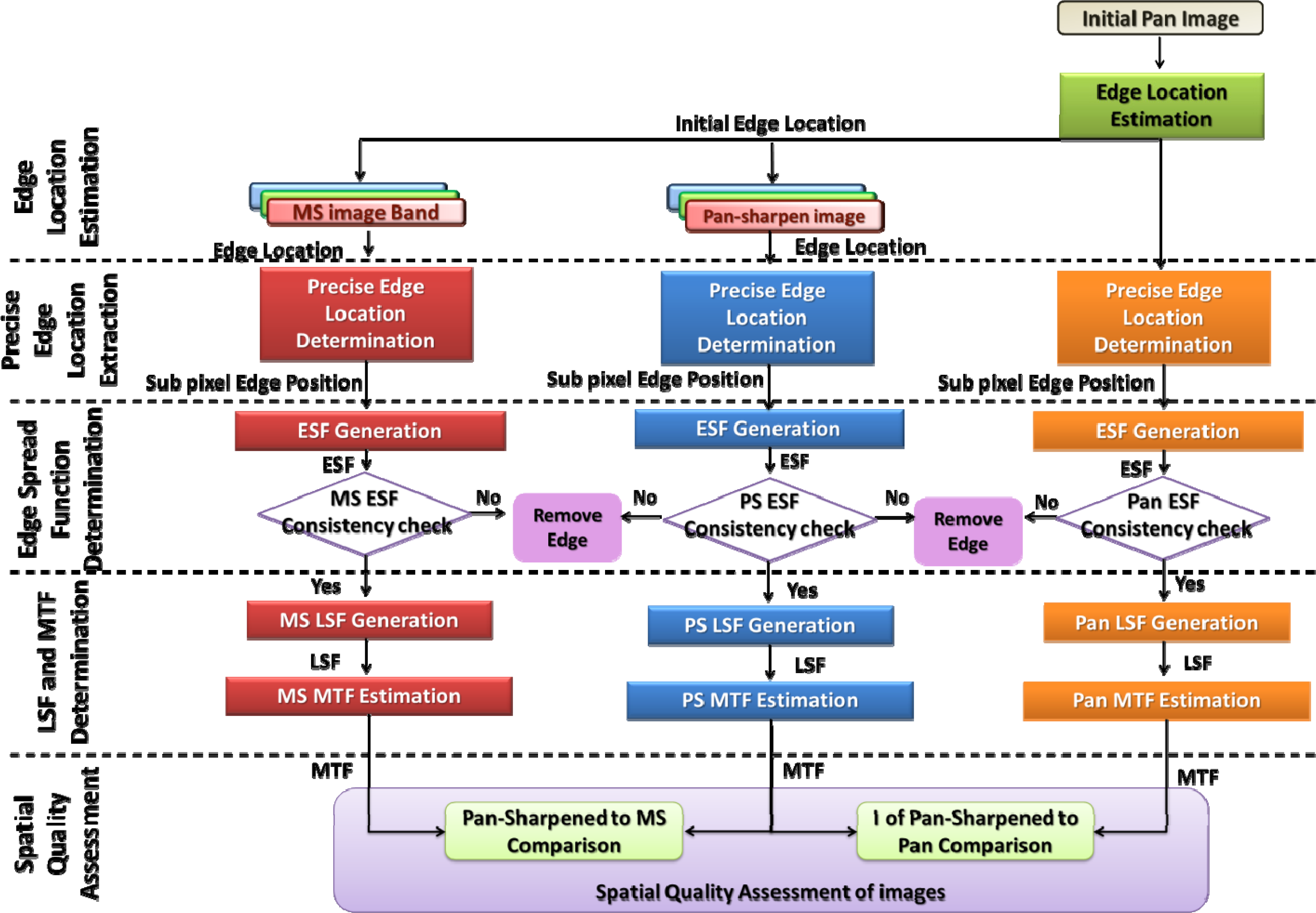
The diagram of the proposed edge-based pan-sharpening spatial quality assessment method is presented in Figure 1. The proposed strategy can be divided into five main steps: edge location estimation, precise edge location extraction, edge spread function determination, LSF, and MTF estimation and spatial quality assessment.

3.1. Edge Location Estimation

Extraction of proper image edges is the first step for the MTF computation. Contrary to the traditional on-orbit MTF computation of satellite imagery, which uses only few specific edges, a variety of edges in different situations should be used to evaluate the quality of edges after the pan-sharpening process. This is due to the fact that, unlike imaging systems, a fusion process does not behave identically for all image edges. High-contrast edges are useful targets for evaluating the spatial response and simulating the image system for all spatial frequencies. For this purpose, the object is usually selected in a way that reflection is high on one side of the edge and is strongly attenuated on the other side. Hence, it is defined as a step edge as stated in Equation (8).

$$\mathit{step}(x,y)=\{\begin{array}{lll}1\hfill & \mathit{if}\hfill & x\ge 0\hfill \\ 0\hfill & \mathit{if}\hfill & x\succ 0\hfill \end{array}$$

(8)

The above function can also be written as [21]:

$$\mathit{step}(x,y)=\mathit{step}(x)=\underset{-\infty }{\overset{x}{\int }}\delta (x)\mathit{dx}=\underset{-\infty }{\overset{x}{\int }}\mathit{line}(x)\mathit{dx}$$

(9)

If the imaging system S is linear, treating the integral as generalized summation yields:

$$\mathit{ESF}(x)=S\{\mathit{step}(x)\}=S\{\underset{-\infty }{\overset{x}{\int }}\delta (x)\mathit{dx}\}=\underset{-\infty }{\overset{x}{\int }}S\{\mathit{line}(x)\}\mathit{dx}=\underset{-\infty }{\overset{x}{\int }}\mathit{LSF}(x)\mathit{dx}$$

(10)

which demonstrates the relationship between an image step edge to ESF and LSF.

Thus, in the first step of the process, all image segments, which have the potentiality to be a good representative of a step image edge, are extracted. To do so, edge extraction operators, such as Canny, are applied on the whole image data set. Then, the direct Hough transform is used to extract the line parameters of all extracted edges.

Amongst the extracted edges, those which are more suitable for spatial quality assessment should be selected. For this purpose, two kinds of evaluation strategies are applied. Firstly, length and slope of the extracted lines are examined and those which are too long, too short, or slanted are removed. The edge profile should be long enough for reliable estimation of the edge behavior; meanwhile, selecting edges that have long profiles may escalate noise effects. To remove too long and too short edges, the contextual situation of imaging scene is taken into consideration. In this situation man-made objects such as buildings and streets are fine objects for finding proper edges for the experiment. Sometimes edges can be detected in the pan-sharpened image, which are not present in the pan-image. These kinds of edges are usually the result of color changes and originate from the multispectral characteristics of the images. Edges which are used in spatial quality evaluation should be extracted from the reference pan-image and then mapped to the generated pan-sharpened and reference images. As the result of this section, candidate edge locations are determined in reference and pan-sharpened images and introduced to the next processing level.

3.2. Precise Edge Location Extraction

This step is dedicated to extract precise sub-pixel edge location. Maximum slope pixels in each extracted edge section are detected line-by-line, applying simple differentiation. To extract sub-pixel edge location, a parametric method is applied. Therefore, the Fermi function is chosen to locate the edge to the sub-pixel location to reduce the estimated MTF error [22]. By inspecting the residuals of fitting Fermi function, the step edges are detected. When the residuals of such least square adjustment are small, it is indicated that the edge shape conforms to Fermi function and typical step edge structure. Edges that are not verified through the mentioned procedure are removed.

After estimation of sub-pixel edge location, least square line fitting to the achieved locations determines the best approximating line. This line minimizes the differences between the edge points on the approximating line and the given edge points values. Solving least square adjustment for all sample points of the edge, line parameters namely slope (a) and intercept (b), are determined (Equation (11)). Based on the computed line parameters, the final edge location can be determined. Figure 2 demonstrates an example of extracted sub-pixel edge locations and the least square line fitted to them.

$$y_i=a.x_i+b$$

(11)

The other evaluation step of extracted edges is the consistency check between each edge location and its degradation from the fitted line equation. It is based on an underlying assumption that the edge of the target lies in a straight line. Thus, edges which suffer from higher residuals in the process of line fitting are compared to a predefined threshold of smallest image element in digital imagery (one pixel) and those exceeding the threshold would be removed from both pan-sharpened and reference images.

3.3. Edge Spread Function Determination

After extracting final edge locations in the previous step, edge profiles are extracted. For each image row, straight lines are constructed perpendicular to the edge and intersecting the edge at sub-pixel positions. In order to obtain enough sample points, selecting the number of data points along the computed ESF is vital. Usually, twenty values are interpolated between two actual data points to build a pseudo-continuous profile in direction perpendicular to the edge line direction [23]. Once the edge profiles have been aligned, it is normally necessary to smooth the data due to potential noise. Several models of ESF can be found in the literature to define a mechanism to avoid noise and aliasing such as cubic splines, sigmoid 3-parameter model, etc. [22–24]. However, Choi and Helder applied Modified Savitzky-Golay (MSG) filter and concluded that MTF errors, at Nyquist frequency, were significantly reduced by using MSG filtering and the Fermi function edge detection strategy [22]. Using original concepts of MSG filter, the best fitting 2D or 4D polynomials are calculated within one pixel window. One point is evaluated by fitting polynomial in the middle of the window. The next value is found by shifting the window by steps of the sub-pixel resolution (0.05 pixel for example) [22].

Generated ESF profiles should pass a consistency check before being introduced to the next steps. This test is crucial to prevent the algorithm from selecting weak or unsteady edges. Thus, in the smoothing step, the deviation of the achieved filtered profiles with respect to the initial samples is evaluated and if it exceeds 99 percent confidence interval (2.5 × σ), the edge will be removed. It should be mentioned that the extracted edges in both reference and pan-sharpened images should be exactly equivalent. Consequently, all edges, which failed in the consistency check, should be removed from all images. Finally, as the results of this section, ESFs of both reference and pan-sharpened images are extracted and introduced to the next section.

3.4. LSF and MTF Estimation

After estimation of the ESF, differentiation is applied to the filtered ESF profile resulting from the previous section. In order to smooth the generated LSF curve and discard the noise, a Gaussian function is adjusted onto the achieved LSF:

$$\mathit{LSF}(x)=\frac{d}{\mathit{dx}}\left[\mathit{ESF}(x)\right]$$

(12)

Discrete Fourier transform of the generated LSF function results in MTF (Equation (13)). The normalized MTF is calculated by dividing the absolute transformed function values by the first absolute value. Following, MTFs for both reference and pan-sharpened images are extracted and introduced to the next section of spatial quality assessment.

$$\mathit{MTF}=\left|\int \mathit{LSF}(x)e^{2\pi \mathit{ix}}\mathit{dx}\right|$$

(13)

3.5. Spatial Quality Assessment

By applying the methods from the four previous sections, MTFs for both reference and processed pan-sharpened images are generated. Now, quality assessment should be performed comparing MTF curves of reference and generated pan-sharpened images. The evaluation process is based on the concept that any edge present in the reference image should appear in the fused image with similar MTF values. The lower degradation of the MTF curve is an indicator of better spatial fusion results.

For quality assessment, two different scenarios are applied. In the first scenario, different fused products are compared to the reference image. As reference image is not always available, we propose to perform a change in scales and to operate at a lower resolution, as promoted by Wald [11]. Accordingly, the initial MS image is considered as the reference image. Thus, spatially down sampled pan- and multi-spectral images are derived and generated from the original ones. In the other scenario, high-resolution fused images are compared with the initial panchromatic image. It is based on the fact that the blurriness of an image is an explicit index of spatial capability of the fusion method in transferring the properties of the reference pan image with high spatial resolution into the processed fused image.

Consequently, we can assess the discrepancies in MTF curves with respect to the reference pan or MS images in each scenario. MTF curves, which exhibit higher values, are more spatially accurate than those with lower values. To compare the MTF curves numerically, the statistical variance index is applied to measure the distance between MTF curves as a final EFM value:

$$\begin{array}{l}{V}_i={\mathit{MTF}}_i^{\mathit{Pan}-\mathit{Sharpened}}-{\mathit{MTF}}_i^{\mathit{reference}}\\ \mathit{Var}=\frac{1}{N}\sum _{i=1}^N{\left(V_i-{\overline{V}}_i\right)}^2\hspace{1em}\text{where}\hspace{1em}\overline{V}={\sum }_{i=1}^N{V}_i/N\\ \mathit{EFM}=1-\mathit{Var}\end{array}$$

(14)

where MTF_i indicates the MTF value at spatial frequency i, N is the total number of spatial sample frequencies, and V̄ is the mean of the variable V_i. In order to be consistent with other measures, EFM is defined in such a way that a higher EFM value refers to a lower difference between pan-sharpened and reference image, which means higher similarity and spatial quality.

4. Experimental Results and Discussion

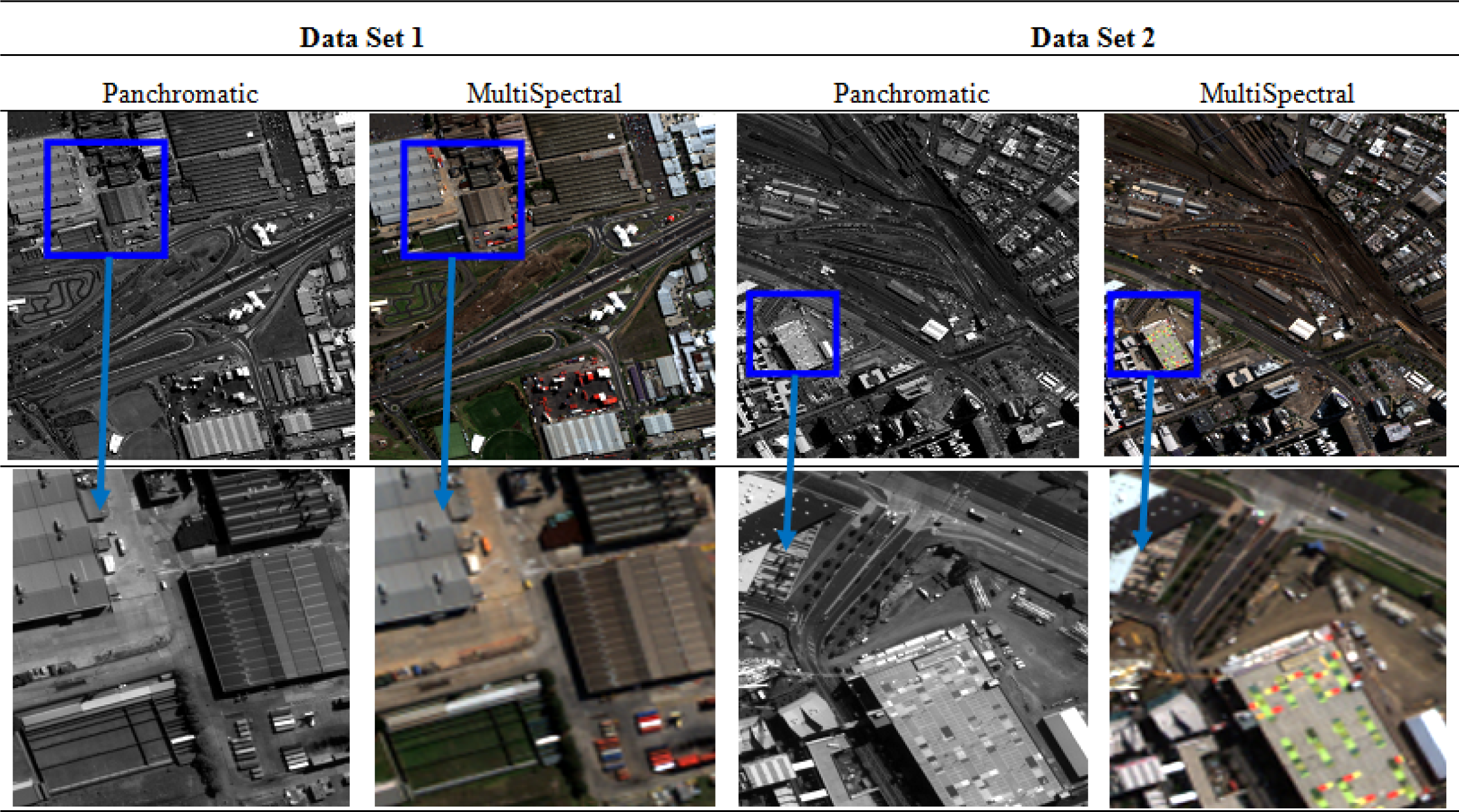
Two different sections of a WorldView-2 high-resolution satellite image data set are used in this experiment, which covers the urban area of Melbourne city (Figure 3). Each data set has eight spectral bands of 500 × 500 pixels and a pan-band of 2000 × 2000 pixels with 2 m and 0.5 m resolution, respectively.

Wavelet and Intensity-Hue-Saturation (IHS) based methods are more common for fusion applications and applied to generate pan-sharpened images. Additive Wavelet Principal Component (AWPC) and Weighted Wavelet Intensity (WWI) methods are selected among the wavelet-based methods and Improved Generalized IHS with Adaptive Weights (IGIHS-AW) and traditional IHS among color based techniques [25–28]. The fundamental relations of the mentioned methods are summarized in

Table 1. Image fusion techniques.

	Method	Equation
1	IHS [25]	$\begin{array}{c}{F}_i={\mathit{MS}}_i+\delta \\ \delta =\mathit{Pan}-I\end{array}$
2	IGIHS-AW [26]	$\begin{array}{c}I=\sum W_i.{\mathit{MS}}_i+\delta \\ F_i=M{S}_i+\frac{{\mathit{MS}}_i}{I}\delta \end{array}$
3	AWPC [27]	$I_{\mathit{new}}=I+\sum _j^3{W}_{{\mathit{Pan}}_j}$
4	WWI [28]	W1 = corr(LLP, LLI) W1 + W2 = 1 W1LLPan + W2LLI

.

Traditional IHS is one of the widely used image fusion techniques. After applying IHS transformation on the MS image, I (intensity) component is replaced by pan [25]. On the other hand, in IGIHS-AW method a synthetic intensity, having a minimum mean square error (MSE) with respect to the reduced pan is computed. The intensity, I, is assumed as a linear combination of MS bands with coefficients (W_i), which are firstly calculated at the spatial scale of the original MS image and a bias (δ), which is computed using a linear regression algorithm [26]. The procedure of AWPC is to transform the RGB components of the multispectral image into the PCA and adding the spatial detail of the panchromatic image to the first principal component [27]. In WWI, a weighted model is used to combine the approximation coefficients of the decomposed pan and I instead of adding details of pan directly to I or totally eliminating the detail coefficients of I (which are related to high frequency information of the image in different scales) [28].

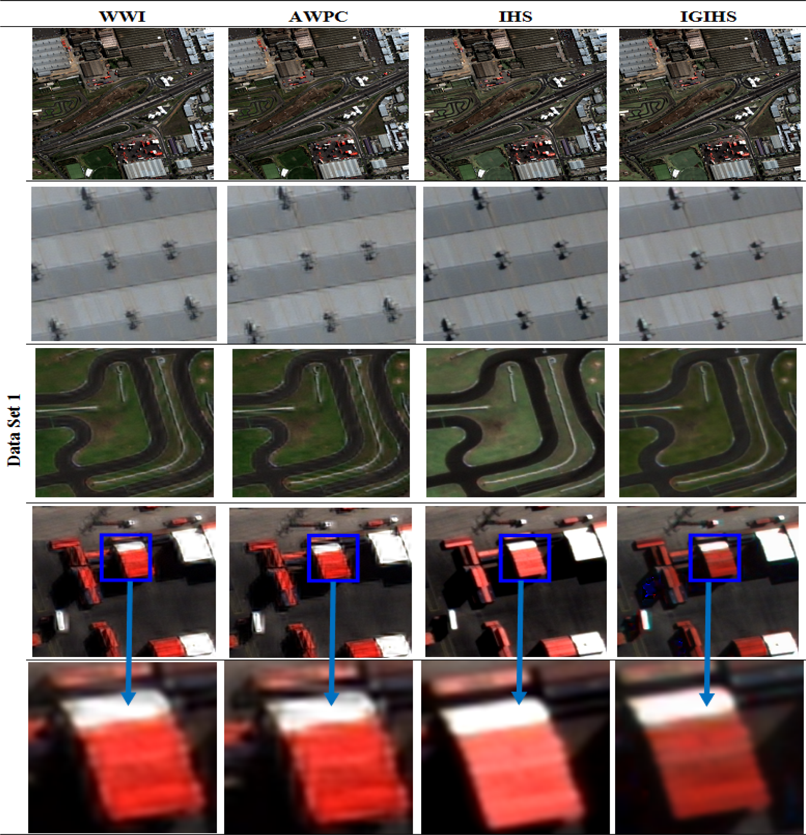
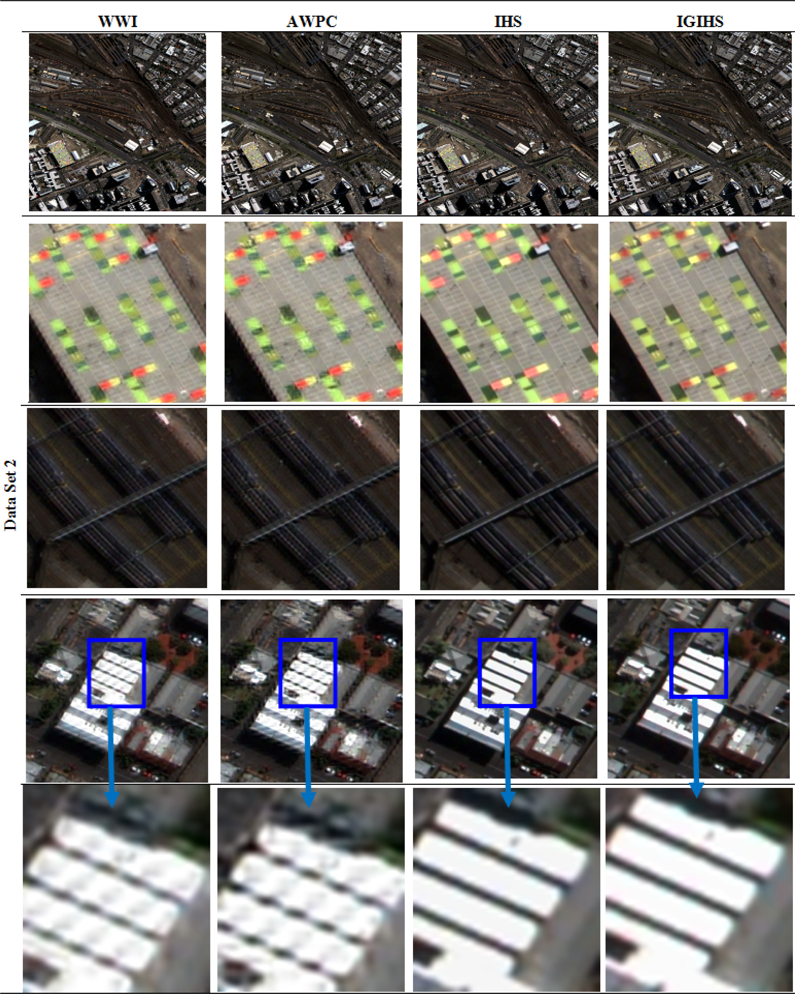
Pan-sharpened images generated by the selected fusion methods for both data sets are presented in Figures 4 and 5. To compare the spatial quality of differently fused images visually, sub-sections (100 × 100 pixels) of the images are extracted and presented.

Visual comparison of the results clearly shows the diversity in spatial quality level of images resulting from different techniques. In addition, in case of wavelet based generated images, tangible spatial distortions are obvious, which means IHS based techniques exhibit superior quality considering spatial distortion.

Two different scenarios for generating reference image have been proposed. In the first scenario, in order to generate a reference image for evaluation based on Wald’s protocol [12], the initial MS image is considered as the reference image, which will be compared to generated pan-sharpened image. Thus, spatially down sampled pan and multispectral images are derived and generated from the original ones by averaging four neighboring pixels of the higher resolution to generate a single value for the down sampled images. The new images have spatial resolution of 2m and 8 m, respectively. Then, they are synthesized at a 2 m resolution applying all four fusion techniques discussed above. The new pan-sharpened image has the resolution of initial multispectral image and is compared to it, which is considered as reference data. For the second evaluation scenario, the intensity band is extracted from R, G, and B bands of the fused image, which are mostly effective on man-made objects and compared to the pan-image. Thus, in this scenario there is no need for rescaling the images.

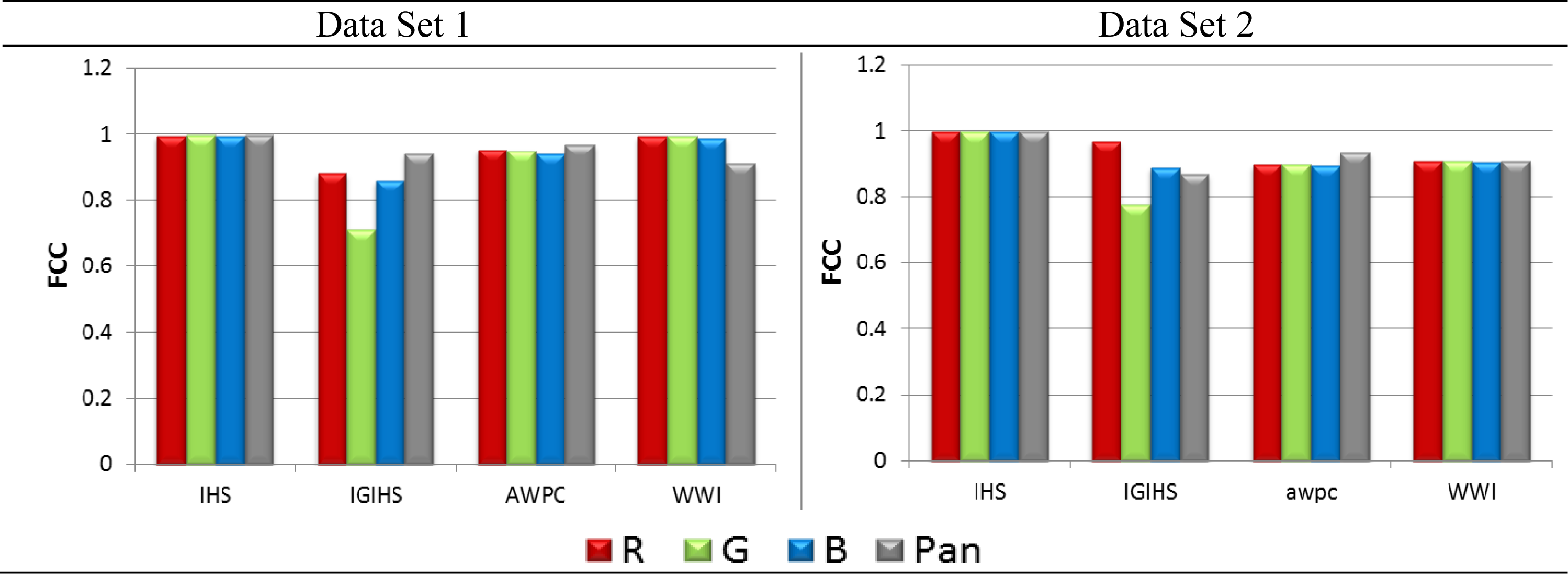
For the possibility of comparing the proposed metric with available methods, the spatial quality of all generated images is evaluated and compared by applying FCC. FCC is one of the most applicable spatial metrics currently proposed [13]. Obtained results are presented in Figure 6, where R, G, and B bands present the results with the first scenario and pan presents results based on the second scenario.

Based on the results depicted in Figure 6, it is clear that the FCC metric is not successful enough in presenting the spatial behavior of fused images. The results, which could be concluded visually from the generated images, are not completely proven by FCC. Firstly it cannot distinguish meaningful differences between different results, which are obvious in Figures 4 and 5. In addition, it is not able to reflect the weakness of wavelet based methods and IGIHS is introduced to be the worse. The reason is that in this method high resolution information is compared based on the correlation index and spatial behavior of image objects is not considered.

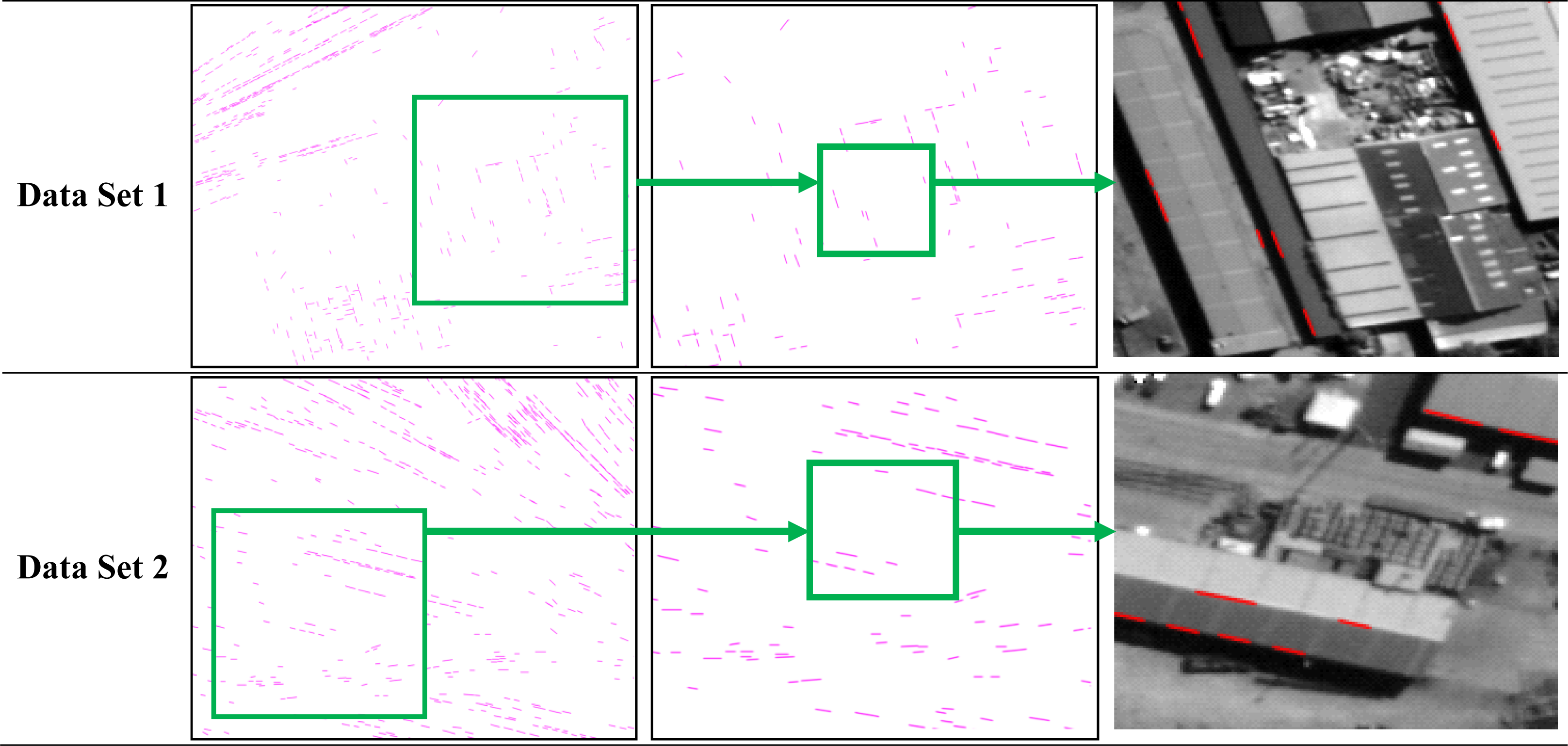
The proposed spatial quality assessment approach is applied on both selected data sets. In the first step, by applying the Canny operator followed by a Hough transform, image edges are extracted for both image data sets. As was discussed previously, to choose appropriate edge candidates, a consistency check is applied on extracted edges and those which appear weak, too short, and too long are removed. Finally, extracted edges are presented in Figure 7. To have a better representation of the results, only parts of images are presented here.

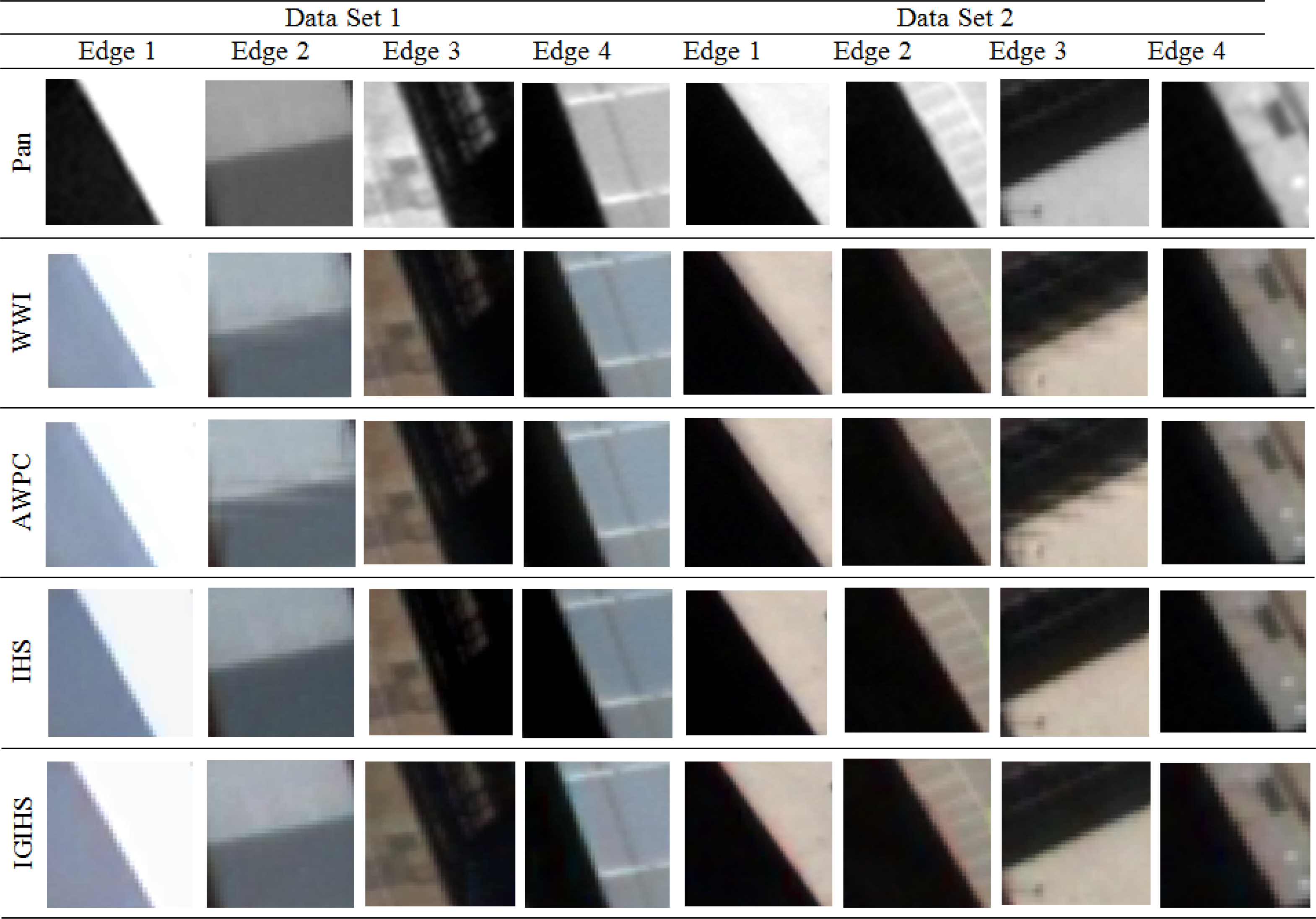
As it has been discussed in the proposed method section, step edges are useful targets for the purpose of image MTF generation. Thus, all edges extracted here are step edges and exhibit proper length and radiometric properties. Four samples of the finally extracted edges in each data set are selected in Figure 8.

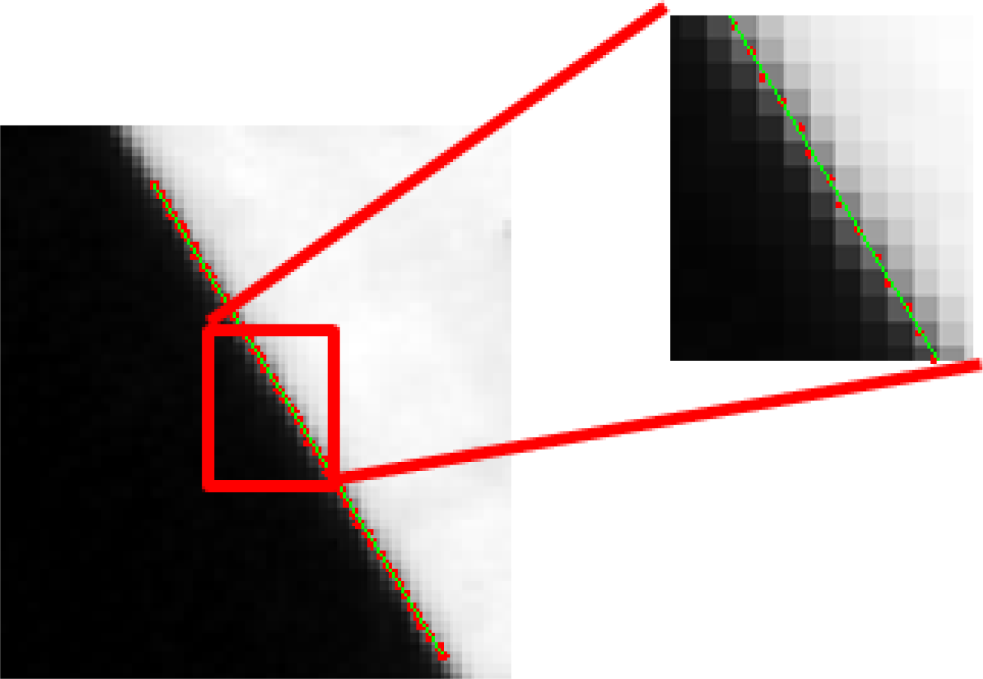
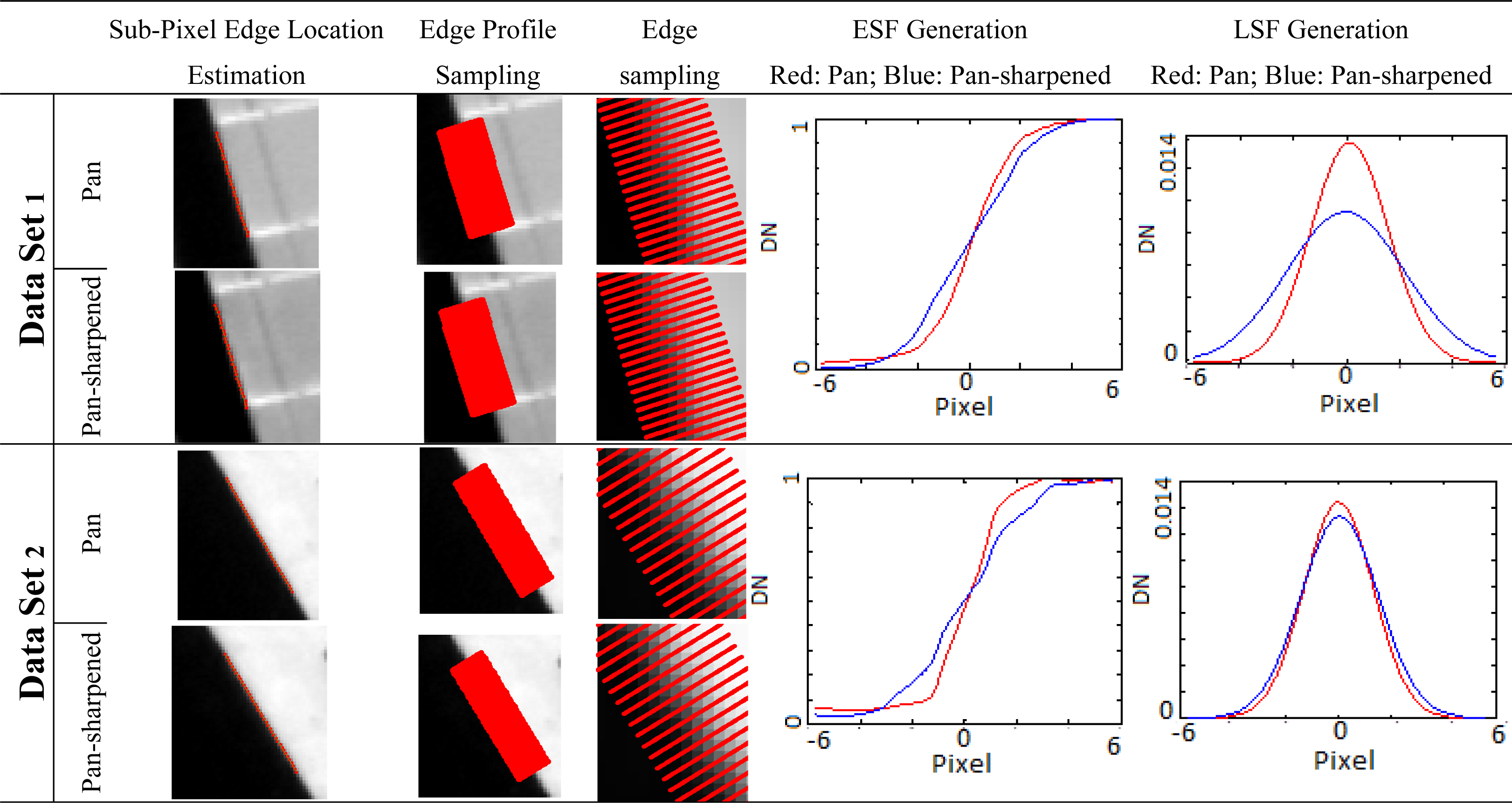
After extraction of edge locations in the image, the sub-pixel edge location can be determined. This process is followed by edge profile extraction. By sampling along the edge, ESF and then LSF profiles are determined as previously described in detail in Section 3. Some snapshots of steps in the LSF computation process are presented in Figure 9.

Figure 9 presents the proposed MTF estimation strategy from sub-pixel edge location estimation to LSF calculation. Following, MTF curves of all generated images are estimated applying Fourier transform of the generated LSF. Figure 10 presents the computed MTF curves for selected edge samples in Figure 8 and compares them to the reference MS image. In this figure, cyan curves present the generated MTF curves for reference images and the others belong to MTF results of the generated pan-sharpened images, each of which has a unique color. Moreover, MTF curves obtained for high-resolution pan and pan-sharpened images based on the second evaluation scenario are also depicted in Figure 11. In this figure, the MTF curves belonging to each pan-sharpened image are presented in a unique color. The MTF of the initial pan-image is presented in black.

Figures 10 and 11 show the differences between pan-sharpened image MTF curves and reference multi-spectral or pan-images. In these figures, the MTF curves located above are more spatially accurate than those located below. Moreover, in these figures as the distance between the MTF curve of the pan-sharpened image and the reference Pan or MS images increases, the less the fusion method is successful in transmitting the high frequencies to rebuild correctly the edges.

Finally the EFM metric is computed for MTF values of edges with respect to the reference images. Achieved results are presented in

Table 2. Closeness of fused and reference multispectral (MS) image Modulation Transfer Function (MTF) values.

		IHS	IGIHS	AWPC	WWI
Data Set 1	R	0.9987	0.9987	0.9984	0.9986
	G	0.9989	0.999	0.9989	0.9987
	B	0.9987	0.9985	0.9982	0.9982
Data Set 2	R	0.9975	0.9974	0.9967	0.9965
	G	0.9986	0.9986	0.9981	0.9979
	B	0.9968	0.9962	0.9959	0.9954

. The results quantify the closeness between original and synthesized MTF curves for each image band separately. Additionally, EFM assessment of resulted pan-sharpened images including comparison to the original pan-image is presented in

Table 3. Closeness of high resolutions fused and initial pan-image MTF values.

	IHS	IGIHS	AWPC	WWI
Data Set 1	0.9999	0.9996	0.9975	0.9973
Data Set 2	0.9996	0.9993	0.9969	0.998

.

All the results obtained show that different image fusion techniques have different spatial behaviors and effects on resulting synthesized images. Although all the values have small changes, they show the diverse behavior of fusion techniques concerning spatial quality. It is also obvious that results with the IHS fusion techniques have the highest closeness values, which mean that IHS has the highest spatial quality compared to the reference images.

On the other hand, concerning lower closeness values of WWI, it could be concluded that this method is the weakest in keeping the spatial quality in its fusion process. In order to compare different fusion techniques, the superiority of spatial quality in image fusion for all extracted edges is rated from 1 to 4 from the weakest to the best spatially fused images and resulted scores from all extracted edges are averaged and normalized. These results are depicted in Figure 12.

This figure shows the comparison of spatial quality of different image fusion techniques while compared to the reference MS image (Red, Green, and Blue). It also compares the quality of the intensity band of fused images with respect to pan-image in different fusion techniques (Gray). This figure indicates that IHS fusion technique has the highest spatial quality while WWI has the lowest one.

To inspect the correctness of results and robustness of the proposed strategy, we also applied Relative Edge Response (RER) index. RER is defined along a given direction, as the difference of the system ESF, at points spaced from the edge by ±0.5 Ground Sampling Distance (GSD). RER can be measured by analyzing the slopes of edge profiles within the image as:

$$\mathit{RER}=\sqrt{[{\mathit{ER}}_x(0.5)-{\mathit{ER}}_x(-0.5)]\hspace{0.17em}\left[{\mathit{ER}}_y(0.5)-{\mathit{ER}}_y(-0.5)\right]}$$

(15)

where ER_x and ER_y refer to the edge response in x and y direction respectively. RER values for all extracted edges are computed and averaged in different image bands of both data sets and results are presented in Figure 13. In this figure, results, which belong to the intensity band of the pan-sharpened image, are dramatically higher because in the second scenario of image evaluation they are compared in the resolution of pan-image and are therefore free from effects of down sampling.

The results depicted in Figure 13 generally show that IHS based methods have better spatial quality in comparison with wavelet based methods in both data sets. This is totally in accordance with those extracted by evaluation of MTF curves based on the proposed strategy and are verified by results of visual comparison of pan-sharpened images.

Comparing all achieved results of FCC metric, the visual comparison of pan-Sharpened images and proposed EFM and RER, it can be concluded that although traditional FCC metric tries to measure spatial similarities between pan-sharpened and reference images, it fails to reflect and measure exact spatial behavior of the generated pan-sharpened images. On the other hand, the proposed EFM, which concentrates on edge response of images, is proven to be more robust and accurate and it could be considered as a powerful and suitable metric for spatial quality assessment of pan-sharpening.

5. Conclusions

Spatial quality assessment of images is as important as spectral quality assessment in object extraction, identification and reconstruction applications in large scale mapping of urban areas especially for man-made objects. There are only few spatial quality assessment methods, which are mainly using edge map comparison, calculated by gradient-like methods. Such methods do not directly measure the spatial characteristics of images and this may lead to wrong conclusions on spatial consistency

This paper has proposed a new edge-based image fusion metric (entitled as EFM) for the evaluation of the spatial quality of pan-sharpened images. The method is based on assessing the spatial response and behavior of the pan-sharpening process by measuring and inspecting edge behavior, which represents the fusion success in transferring spatial data from the higher resolution image into the pan-sharpened image. EFM automatically extracts the MTF of pan-sharpened images and compares it to the MTF of reference images. Unlike traditional MTF computation of satellite imagery, which uses only few specific edges, in the proposed method various strong edges in different situations are used to evaluate the robustness of edge transposition into pan-sharpened image. Moreover, lots of evaluation steps are assumed which help preserving the algorithm from noise, unsteady or false results.

The proposed fusion quality assessment strategy provides the capability of spatial quality assessment of different fusion techniques or products. Comparing the obtained results, it can be concluded that the proposed EFM is robust and accurate for spatial evaluation, assessment, and comparison of fused images. EFM is also more sensitive to spatial degradations of pan-sharpened images than traditional FCC method and it can be applied as an efficient assessment metric. It is able to compare different fusion methods and assess fusion products, which are more spatially similar to the reference image. Moreover, EFM provides producers with the valuable chance of choosing proper fusion methods and users to decide about the quality of pan-sharpened products. Additionally, the proposed strategy depends on the precise extraction of edges and any shortcoming in this step would affect all other computation and the final results. Moreover, in data sets lacking robust and appropriate edges, the proposed method might appear weak and it is recommended to use PSF instead of LSF for generation MTF curves.