Application of a Land Surface Model Using Remote Sensing Data for High Resolution Simulations of Terrestrial Processes

Abstract
:1. Introduction
2. Model Description
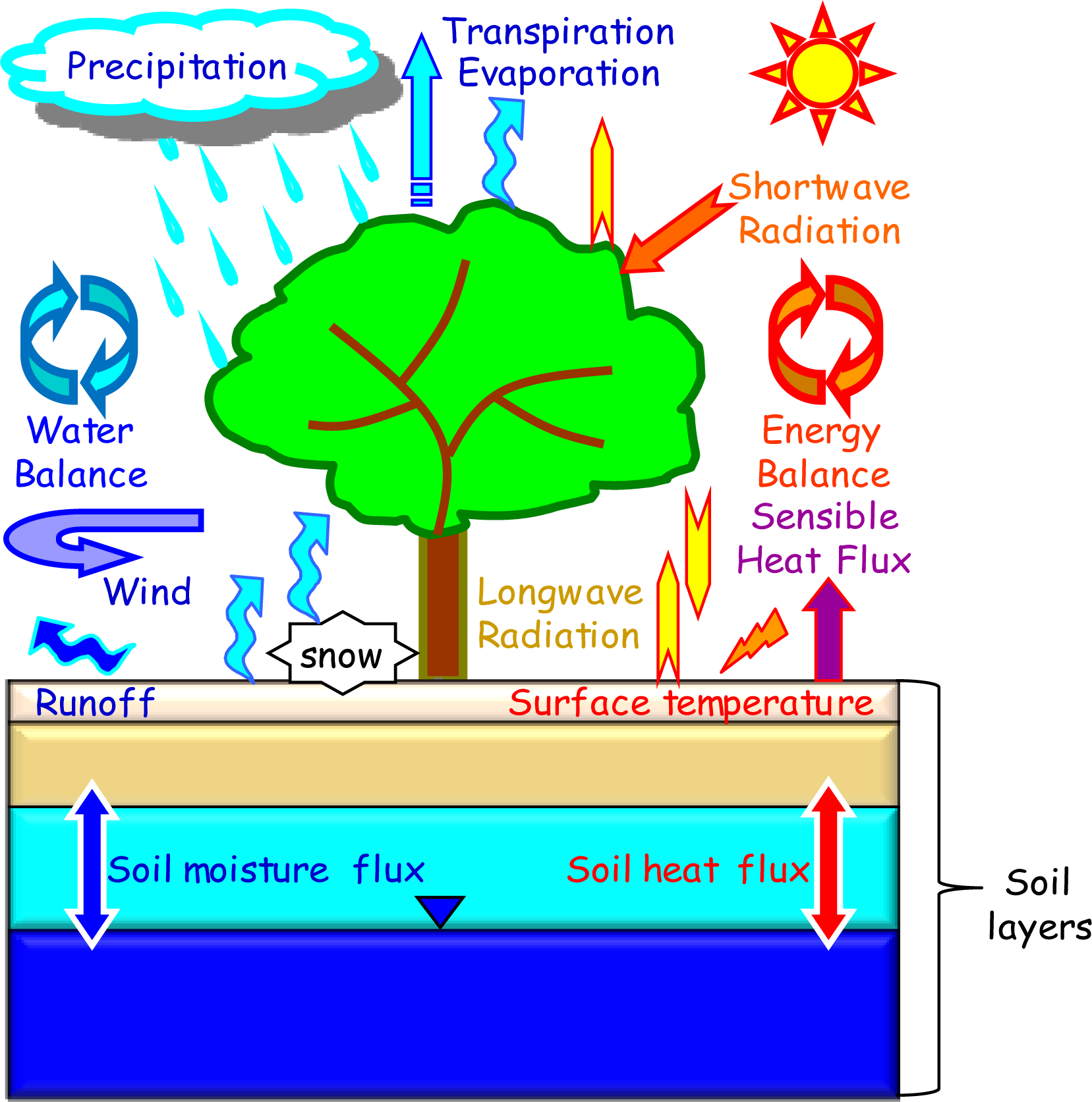
2.1. General Description on CoLM
2.1. Runoff Simulation Scheme
2.3. Soil Temperature Simulation Scheme
3. Model Setup
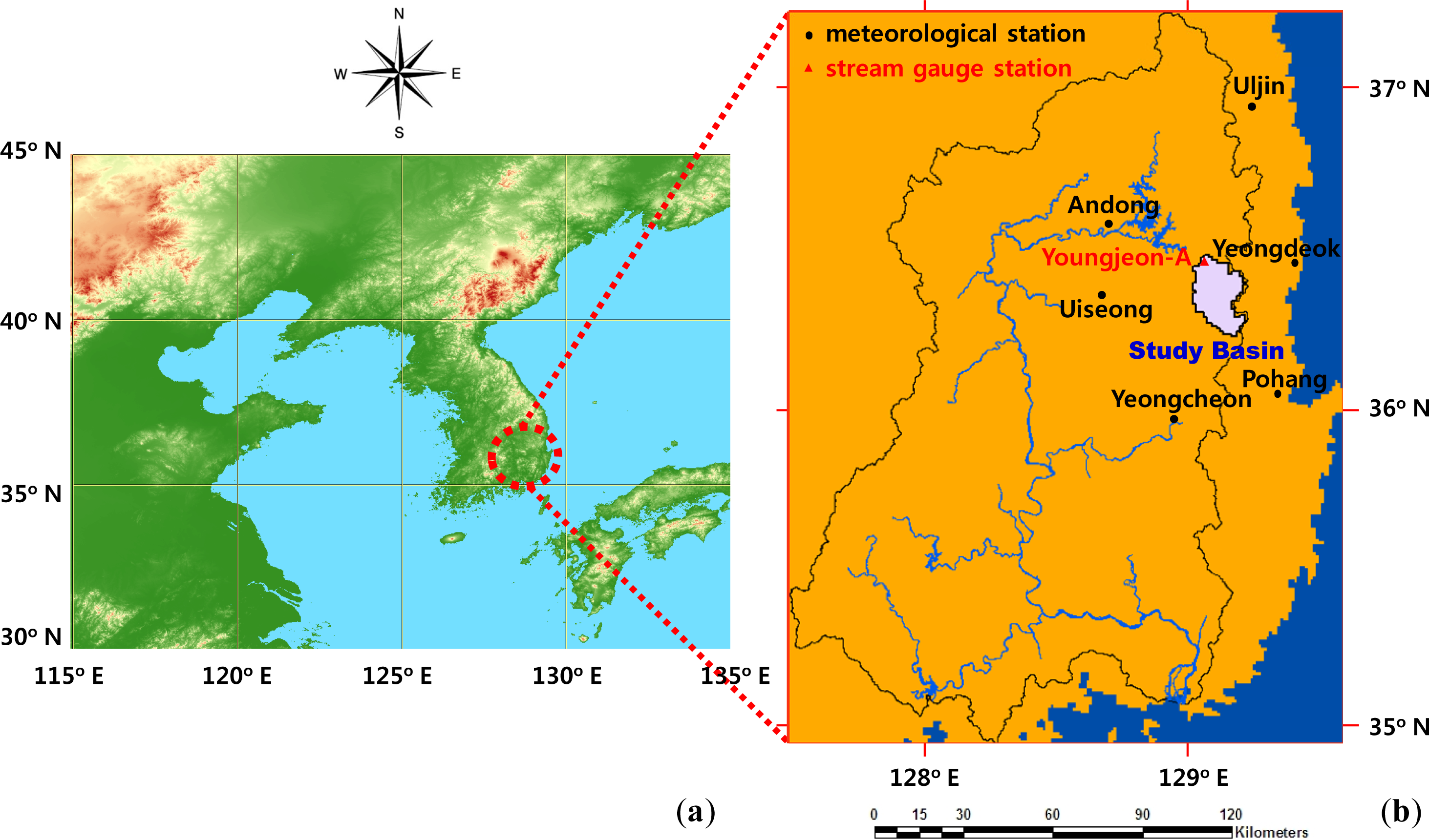
3.1. Study Basin
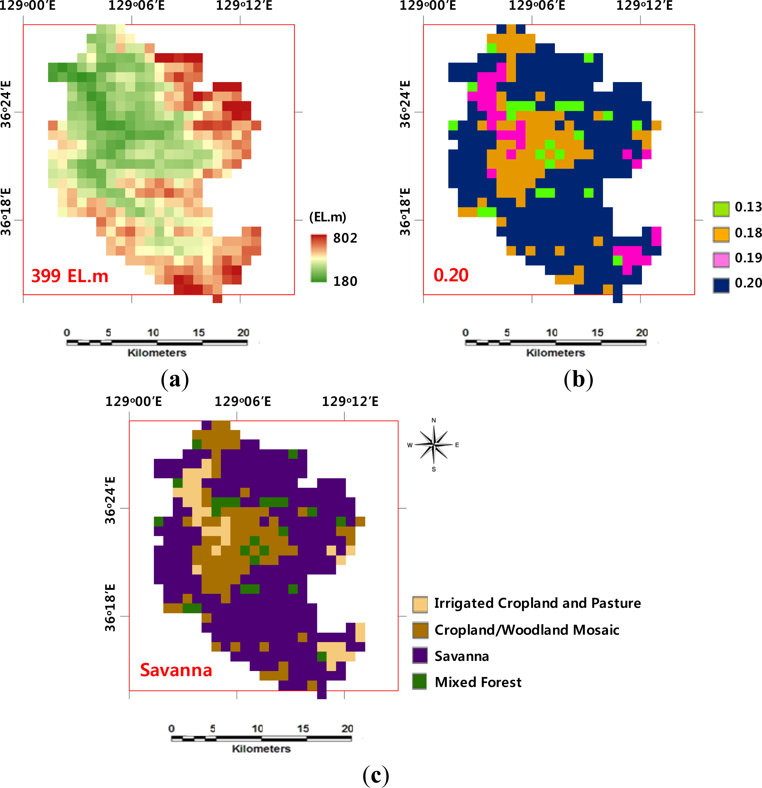
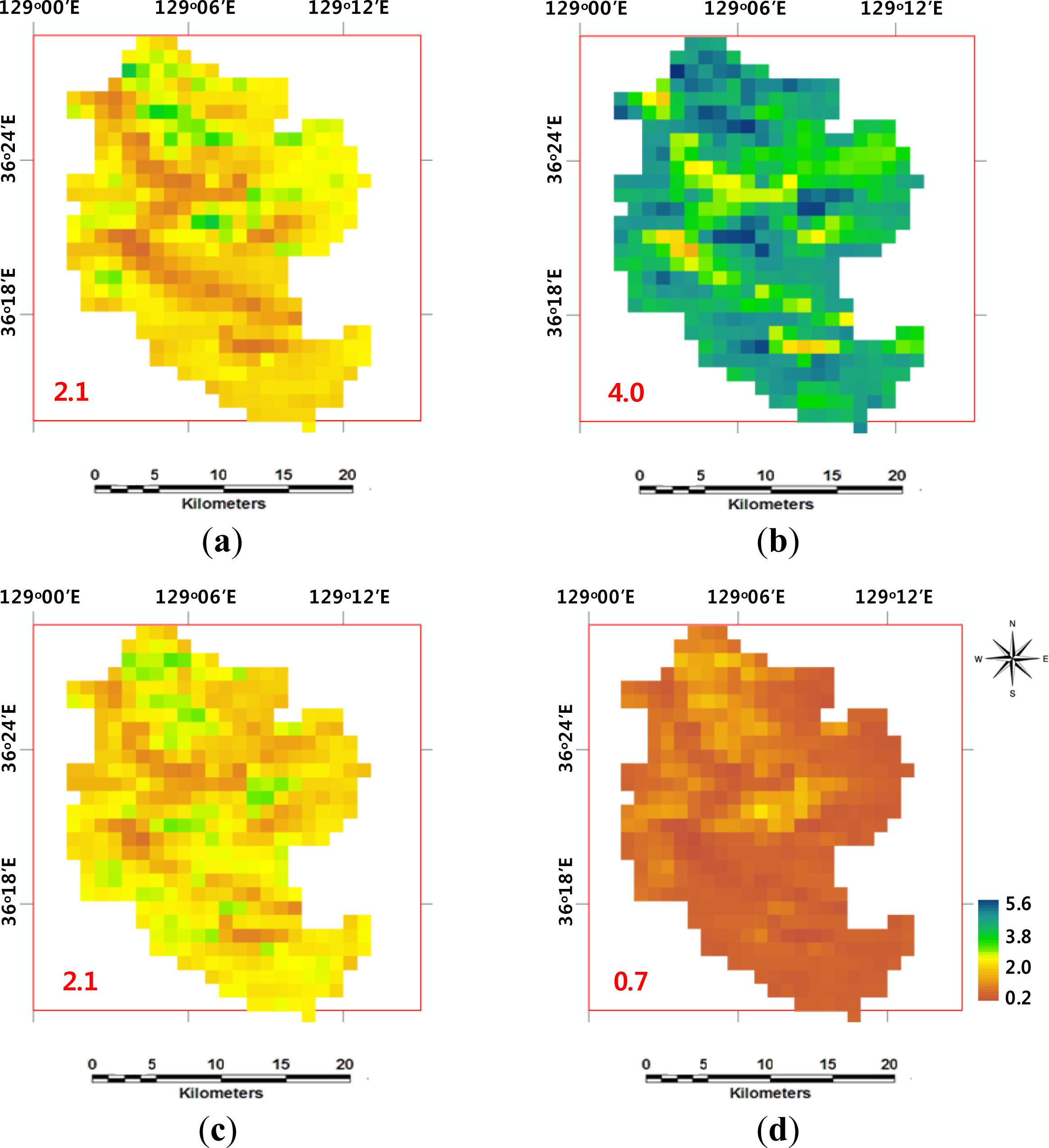
3.2. Surface Boundary Conditions
3.3. Meteorological Forcing and Initial Conditions
4. Results and Discussion
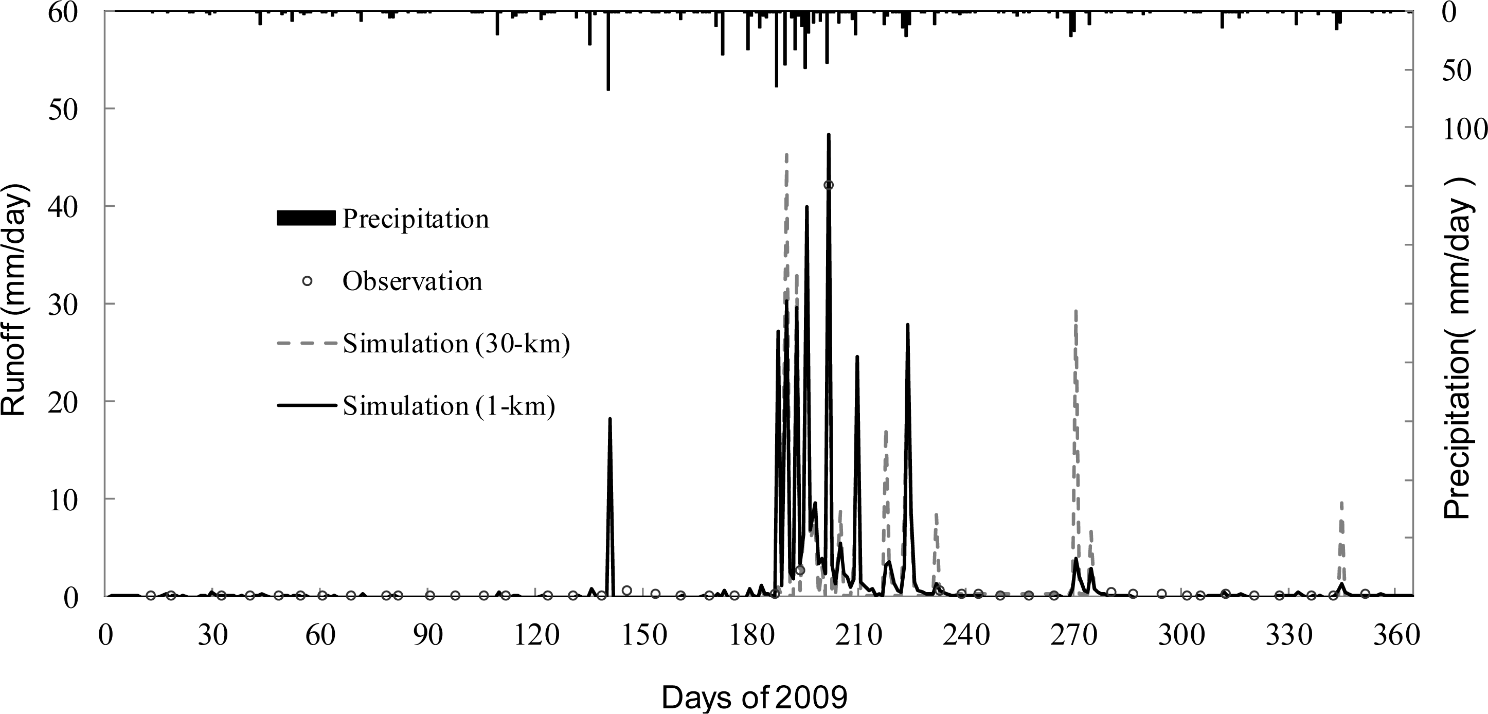
4.1. Runoff Results
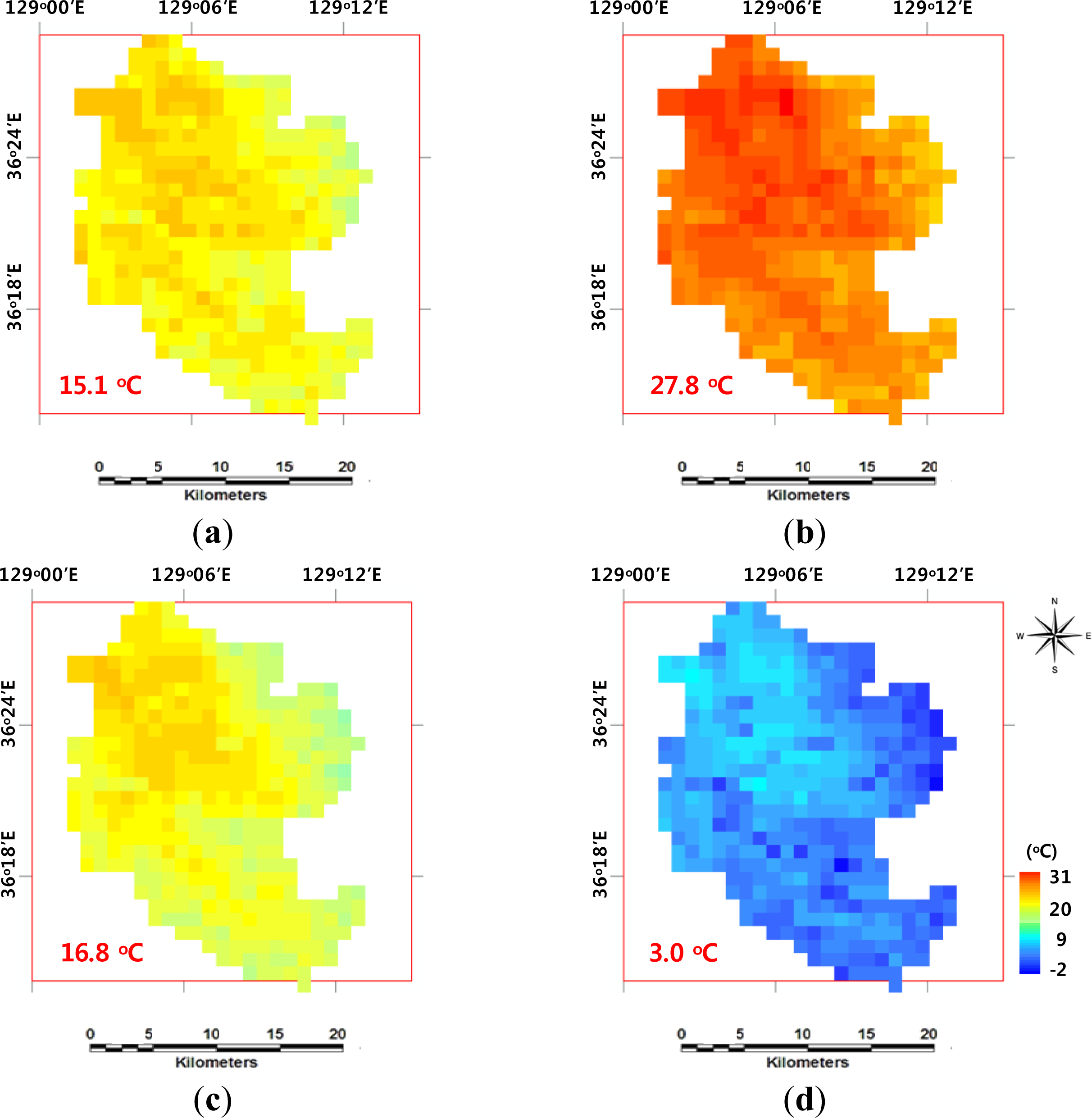
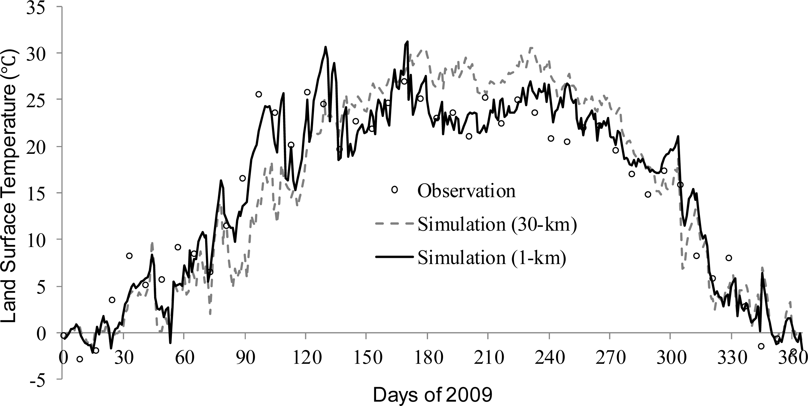
4.2. Land Surface Temperature Results
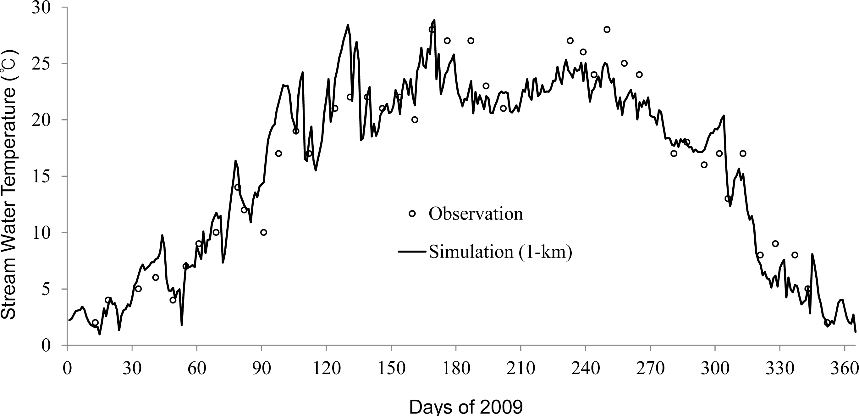
4.3. Stream Water Temperature Estimations
5. Conclusions
Acknowledgments
Conflicts of Interest
References
- Bates, B.C.; Kundzewicz, Z.W.; Wu, S.; Palutikof, J.P. Climate Change and Water; Technical Paper of Intergovernmental Panel on Climate Change; IPCC Secretariat: Geneva, Switzerland, 2008; p. 210. [Google Scholar]
- Stieglitz, M.; Rind, D.; Famiglietti, J.; Rosenzweig, C. An efficient approach to modeling the topographic control of surface hydrology for regional modeling. J. Clim 1997, 10, 118–137. [Google Scholar]
- Chen, J.; Kumar, P. Topographic influence of the seasonal and interannual variation of water and energy balance of basins in North America. J. Clim 2001, 14, 1989–2014. [Google Scholar]
- Warrach, K.; Stieglitz, M.; Mengelkamp, H.-T.; Raschke, E. Advantages of a topographically controlled runoff simulation in a soil-vegetation-atmosphere transfer model. J. Hydrometeorol 2002, 3, 131–148. [Google Scholar]
- Niu, G.-Y.; Yang, Z.-L. The versatile integrator of surface and atmosphere processes (VISA) Part II: Evaluation of three topography based runoff schemes. Global Planet. Change 2003, 38, 191–208. [Google Scholar]
- Niu, G.-Y.; Yang, Z.-L.; Dickinson, R.E.; Gulden, L.E. A simple TOPMODEL-based runoff parameterization (SIMTOP) for use in GCMs. J. Geophys. Res 2005, 110, D21106. [Google Scholar]
- Oleson, K.W.; Niu, G.-Y.; Yang, Z.-L.; Lawrence, D.M.; Thornton, P.E.; Lawrence, P.J.; Stockli, R.; Dickinson, R.E.; Bonan, G.B.; Levis, S.; et al. Improvements to the community land model and their impact on the hydrological cycle. J. Geophys. Res 2008, 113, G01021. [Google Scholar]
- Choi, H.I.; Liang, X.-Z. Improved terrestrial hydrologic representation in mesoscale land surface models. J. Hydrometeorol 2010, 11, 797–809. [Google Scholar]
- Dai, Y.; Zeng, X.; Dickinson, R.E.; Baker, I.; Bonan, G.B.; Bosilovich, M.G.; Denning, A.S.; Dirmeyer, P.A.; Houser, P.R.; Niu, G.; et al. The common land model. Bull. Am. Meteorol. Soc 2003, 84, 1013–1023. [Google Scholar]
- Liang, X.-Z.; Li, L.; Dai, A.; Kunkel, K.E. Regional climate model simulation of summer precipitation diurnal cycle over the United States. Geophys. Res. Lett 2004, 31, L24208. [Google Scholar]
- Liang, X.-Z.; Xu, M.; Zhu, J.; Kunkel, K.E.; Wang, J.X.L. Development of the Regional Climate-Weather Research and Forecasting Model (CWRF): Treatment of Topography. Proceedings of the 2005 WRF/MM5 User’s Workshop, Boulder, CO, USA, 27–30 June 2005; p. 5.
- Liang, X.-Z.; Xu, M.; Yuan, X.; Ling, T.; Choi, H.I.; Zhang, F.; Chen, L.; Liu, S.; Su, S.; Qiao, F.; et al. Regional climate-weather research and forecasting model. Bull. Am. Meteorol. Soc 2012, 93, 1363–1380. [Google Scholar]
- Niu, G.-Y.; Yang, Z.-L. Effects of frozen soil on snowmelt runoff and soil water storage at a continental scale. J. Hydrometeorol 2006, 7, 937–952. [Google Scholar]
- Qian, T.; Dai, A.; Trenberth, K.E.; Oleson, K.W. Simulation of global land surface conditions from 1948 to 2004: Part I: Forcing data and evaluations. J. Hydrometeorol 2006, 7, 953–975. [Google Scholar]
- Choi, H.I.; Kumar, P.; Liang, X.-Z. Three-dimensional volume-averaged soil moisture transport model with a scalable parameterization of subgrid topographic variability. Water Resour. Res 2007, 43, W04414. [Google Scholar]
- Niu, G.-Y.; Yang, Z.-L.; Dickinson, R.E.; Gulden, L.E.; Su, H. Development of a simple groundwater model for use in climate models and evaluation with gravity recovery and climate experiment data. J. Geophys. Res 2007, 112, D07103. [Google Scholar]
- Lawrence, P.J.; Chase, T.N. Representing a new MODIS consistent land surface in the Community Land Model (CLM3.0). J. Geophys. Res 2007, 112, G01023. [Google Scholar]
- Lawrence, D.M.; Thornton, P.E.; Oleson, K.W.; Bonan, G.B. The partitioning of evapotranspiration into transpiration, soil evaporation, and canopy evaporation in a GCM: Impacts on land-atmosphere interaction. J. Hydrometeorol 2007, 8, 862–880. [Google Scholar]
- Kim, E.S.; Choi, H.I.; Kim, S. Implementation of a topographically controlled runoff scheme for land surface parameterizations in regional climate models. KSCE J. Civil Eng 2011, 15, 1309–1318. [Google Scholar]
- Liang, X.-Z.; Choi, H.L.; Kunkel, K.E.; Dai, Y.; Joseph, E.; Wang, J.X.L.; Kumar, P. Surface boundary conditions for mesoscale regional climate models. Earth Interact 2005, 9, 1–28. [Google Scholar]
- Liang, X.-Z.; Xu, M.; Gao, W.; Kunkel, K.E.; Slusser, J.; Dai, Y.; Min, Q.; Houser, P.R.; Rodell, M.; Schaaf, C.B.; et al. Development of land surface albedo parameterization bases on Moderate Resolution Imaging Spectroradiometer (MODIS) data. J. Geophys. Res 2005, 110, D11107. [Google Scholar]
- Gao, W.; Gao, Z.Q.; Choi, H.I.; Xu, M.; Slusser, J.R. Construction of surface boundary conditions for regional climate modeling in China by using the remote sensing data. Proc. SPIE 2005, 5884, 331–335. [Google Scholar]
- Choi, H.I. Use of sensor imagery data for surface boundary conditions in regional climate modeling. Sensors 2011, 11, 6728–6742. [Google Scholar]
- Choi, H.I. Parameterization of high resolution vegetation characteristics using remote sensing products for the Nakdong River Watershed, Korea. Remote Sens 2013, 5, 473–490. [Google Scholar]
- Beven, K.J.; Kirkby, M.J. A physically based, variable contributing area model of basin hydrology. Hydrol. Sci. Bull 1979, 24, 43–69. [Google Scholar]
- Beven, K.J. On subsurface stormflow: An analysis of response times. Hydrol. Sci. J 1982, 27, 505–521. [Google Scholar]
- Beven, K.J. Infiltration into a class of vertically non-uniform soils. Hydrol. Sci. J 1984, 29, 425–434. [Google Scholar]
- Elsenbeer, H; Cassel, D.K.; Castro, J. Spatial analysis of soil hydraulic conductivity in a tropical rainforest catchment. Water Resour. Res 1992, 28, 3201–3214. [Google Scholar]
- Beven, K.J. Macropores and water flow in soils. Water Resour. Res 1982, 18, 1311–1325. [Google Scholar]
- Brooks, R.H.; Corey, A.T. Hydraulic Properties in Porous Media; Hydrology Paper No. 3; Colorado State University: Fort Collins, CO, USA, 1964; p. 27. [Google Scholar]
- STRM 90m DEM Database V4.1. Consortium for Spatial Information (CSI), Consultative Group on International Agricultural Research (CGIAR): Washington, DC, USA, 2008. Available online: http://www.cgiar-csi.org/data/srtm-90m-digital-elevation-database-v4-1 (accessed on 30 September 2013).
- FAO-IIASA. Harmonized World Soil Database (version 1.2); FAO: Rome, Italy; IIASA: Laxenburg, Austria, 2012. [Google Scholar]
- GLCC Database. US Department of the Interior, US Geological Survey: Washington, DC, USA. Available online: http://edc2.usgs.gov/glcc/glcc.php (accessed on 30 September 2013).
- AVHRR NDVI Database. US Department of the Interior, US Geological Survey: Washington, DC, USA. Available online: http://phenology.cr.usgs.gov/ndvi_avhrr.php (accessed on 30 September 2013).
- Zeng, X.; Dickinson, R.E.; Walker, A.; Shaikh, M.; DeFries, R.S.; Qi, J. Derivation and evaluation of global 1–km fractional vegetation cover data for land modeling. J. Appl. Meteorol 2000, 39, 826–839. [Google Scholar]
- Zeng, X.; Shaikh, M.; Dai, Y.; Dickinson, R.E.; Myneni, R. Coupling of the common land model to the NCAR community climate model. J. Clim 2002, 15, 1832–1854. [Google Scholar]
- Free VEGETATION Products. VITO: Belgium. Available online: http://free.vgt.vito.be (accessed on 30 September 2013).
- MOD 15 LAI Data. US Geological Survey: Reston, VA, USA. Available online: https://lpdaac.usgs.gov/get_data (accessed on 30 September 2013).
- Yucel, I. Effects of implementing MODIS land cover and albedo in MM5 at two contrasting US regions. J. Hydrometeorol 2006, 7, 1043–1060. [Google Scholar]
- Nash, J.E.; Sutcliffe, J.V. River flow forecasting through conceptual models part I-A discussion of principles. J. Hydrol 1970, 10, 282–290. [Google Scholar]
- Choi, H.I.; Liang, X.-Z.; Kumar, P. A conjunctive surface–Subsurface flow representation for mesoscale land surface models. J. Hydrometeorol 2013, 14, 1421–1442. [Google Scholar]


| Variable | Unit |
|---|---|
| pressure at the lowest atmospheric layer | Pa |
| temperature at the lowest atmospheric layer | K |
| specific humidity at the lowest atmospheric layer | kg/kg |
| zonal wind at the lowest atmospheric layer | m/s |
| meridional wind at the lowest atmospheric layer | m/s |
| the lowest atmospheric layer height | m |
| pressure at surface | Pa |
| convective rainfall | mm |
| resolved rainfall | mm |
| snow | mm |
| planetary boundary layer height | m |
| downward long wave radiation onto the surface | W/m2 |
| downward short wave flux at ground surface | W/m2 |
| Rbas,max = 1 ×10⁻⁴ | Rbas,max = 2 × 10⁻⁴ | Rbas,max = 3 × 10⁻⁴ | Rbas,max = 4 × 10⁻⁴ | ||||||
|---|---|---|---|---|---|---|---|---|---|
| NSC | MAE | NSC | MAE | NSC | MAE | NSC | MAE | ||
| 1-km | f = 2 | 0.989 | 0.226 | 0.990 | 0.210 | 0.989 | 0.202 | 0.990 | 0.197 |
| f = 4 | 0.993 | 0.203 | 0.994 | 0.205 | 0.991 | 0.220 | 0.991 | 0.214 | |
| f = 6 | 0.997 | 0.174 | 0.996 | 0.192 | 0.991 | 0.229 | 0.993 | 0.218 | |
| f = 8 | 0.997 | 0.186 | 0.995 | 0.207 | 0.995 | 0.209 | 0.992 | 0.224 | |
| 30-km | f = 2 | 0.958 | 0.463 | 0.958 | 0.490 | 0.959 | 0.481 | 0.960 | 0.443 |
| f = 4 | 0.959 | 0.367 | 0.957 | 0.405 | 0.959 | 0.370 | 0.959 | 0.365 | |
| f = 6 | 0.961 | 0.354 | 0.960 | 0.364 | 0.959 | 0.368 | 0.959 | 0.362 | |
| f = 8 | 0.959 | 0.361 | 0.959 | 0.370 | 0.958 | 0.386 | 0.958 | 0.410 | |
| Rbas,max = 1 × 10⁻⁴ | Rbas,max = 2 × 10⁻⁴ | Rbas,max = 3 × 10⁻⁴ | Rbas,max = 4 × 10⁻⁴ | ||||||
|---|---|---|---|---|---|---|---|---|---|
| NSC | MAE | NSC | MAE | NSC | MAE | NSC | MAE | ||
| 1-km | f = 2 | 0.832 | 2.632 | 0.830 | 2.648 | 0.829 | 2.651 | 0.830 | 2.645 |
| f = 4 | 0.860 | 2.366 | 0.859 | 2.376 | 0.859 | 2.378 | 0.859 | 2.376 | |
| f = 6 | 0.868 | 2.258 | 0.868 | 2.261 | 0.868 | 2.263 | 0.868 | 2.261 | |
| f = 8 | 0.866 | 2.270 | 0.866 | 2.269 | 0.866 | 2.269 | 0.866 | 2.269 | |
| 30-km | f = 2 | 0.669 | 3.957 | 0.667 | 3.975 | 0.668 | 3.965 | 0.671 | 3.923 |
| f = 4 | 0.673 | 3.888 | 0.673 | 3.891 | 0.672 | 3.906 | 0.672 | 3.898 | |
| f = 6 | 0.675 | 3.883 | 0.675 | 3.883 | 0.675 | 3.883 | 0.675 | 3.883 | |
| f = 8 | 0.673 | 3.898 | 0.673 | 3.898 | 0.673 | 0.898 | 0.672 | 3.899 | |
© 2013 by the authors; licensee MDPI, Basel, Switzerland This article is an open access article distributed under the terms and conditions of the Creative Commons Attribution license ( http://creativecommons.org/licenses/by/3.0/).
Share and Cite
Choi, H.I. Application of a Land Surface Model Using Remote Sensing Data for High Resolution Simulations of Terrestrial Processes. Remote Sens. 2013, 5, 6838-6856. https://doi.org/10.3390/rs5126838
Choi HI. Application of a Land Surface Model Using Remote Sensing Data for High Resolution Simulations of Terrestrial Processes. Remote Sensing. 2013; 5(12):6838-6856. https://doi.org/10.3390/rs5126838
Chicago/Turabian StyleChoi, Hyun Il. 2013. "Application of a Land Surface Model Using Remote Sensing Data for High Resolution Simulations of Terrestrial Processes" Remote Sensing 5, no. 12: 6838-6856. https://doi.org/10.3390/rs5126838