A Voxel-Based Method for Automated Identification and Morphological Parameters Estimation of Individual Street Trees from Mobile Laser Scanning Data

 ,
, 
Abstract
: As an important component of urban vegetation, street trees play an important role in maintenance of environmental quality, aesthetic beauty of urban landscape, and social service for inhabitants. Acquiring accurate and up-to-date inventory information for street trees is required for urban horticultural planning, and municipal urban forest management. This paper presents a new Voxel-based Marked Neighborhood Searching (VMNS) method for efficiently identifying street trees and deriving their morphological parameters from Mobile Laser Scanning (MLS) point cloud data. The VMNS method consists of six technical components: voxelization, calculating values of voxels, searching and marking neighborhoods, extracting potential trees, deriving morphological parameters, and eliminating pole-like objects other than trees. The method is validated and evaluated through two case studies. The evaluation results show that the completeness and correctness of our method for street tree detection are over 98%. The derived morphological parameters, including tree height, crown diameter, diameter at breast height (DBH), and crown base height (CBH), are in a good agreement with the field measurements. Our method provides an effective tool for extracting various morphological parameters for individual street trees from MLS point cloud data.1. Introduction
Urban vegetation is an important component of urban ecosystem and landscape. In particular, street trees play an important role in enhancing environmental quality, maintaining aesthetic beauty of urban landscape, and providing social service for inhabitants. Street trees provide shade for pedestrians, benefit storm-water management [1], reduce air pollutants [2–4] and street noise [5], moderate heat accumulation in urban street canyons [6–8], and decrease building energy consumption and CO2 emissions [9]. However, the growth conditions of street trees are often negatively influenced by some natural and abiotic factors [10]. Some studies show that about half of newly transplanted street trees cannot survive beyond the first two years in some cities [11,12]. Therefore, acquiring and monitoring the conditions of street trees is important for urban tree planting, maintenance, and management.
A comprehensive inventory and classification of street trees need multiple characteristic parameters: tree species, growth conditions, presence or absence of insects or diseases, transplantation requirements, date of planting, etc. [10]. The growth condition and biological function of an individual tree can be inferred from its morphological parameters, such as tree height, diameter at breast height (DBH), crown width, and crown base height (CBH). Traditionally, these parameters of street trees are obtained by field measurements, which are very time-consuming and labor is expensive. Since the size and shape of street trees are changing from year to year, even from season to season, it would be extremely costly to acquire the up-to-date street tree information with the field measurement method. A more efficient method is needed for deriving information about urban street trees.
The advent of the laser scanning or LiDAR (Light Detection and Ranging) system represents a technological breakthrough in acquiring three-dimensional (3D) data about surface objects in a rapid, and cost-effective manner. In terms of the carrying platform, laser scanning systems can be classified into four categories: Satellite-based Laser Scanning (SLS), Airborne Laser Scanning (ALS, namely, airborne LiDAR), Mobile Laser Scanning (MLS, in full, Vehicle-borne Laser Scanning, VLS), and Terrestrial Laser Scanning (TLS). The SLS data have sparse sampling points and are not adequate for street tree identification [13]. TLS data have the highest accuracy and sampling density and can be used for structure reconstruction of individual trees [14–16]. However, the poor mobility of TLS restricts repeated surveys for a large urban area. ALS has the extraordinary capability in gathering highly accurate and dense elevation measurements. Numerous studies demonstrate that ALS data can be employed to investigate urban 3D morphology [17], to extract building rooftops, footprints, and density information [18–21], to estimate urban green volume [22,23], and to detect individual trees [24–26]. Nevertheless, due to the top-down sensing geometry, it is difficult for ALS to capture the side-view geometry of a tree or to detect the structures under tree crowns. Some tree morphological parameters, such as DBH and CBH, are very difficult to be derived from ALS data.
As a new mobile mapping system, MLS allows for quick and cost-effective acquisition of close-range 3D measurements of street objects [27–30]. MLS has been used for modeling road surfaces [31], extracting building facades [29,32–34], and detecting trees, streetlights, and other pole-like objects [28,35–37]. Previous studies have demonstrated the great potential of MLS for street objects identification.
Although many data processing and objects classification methods have been developed for ALS data, not much research work has been reported on methods and software tools for processing MLS data. ALS records the geometric information about rooftop structure of objects from the top, whereas MLS views the objects from the side and can record the geometric information about the building facades under the rooftop as well as the trunk of a tree under the crown. Due to differences in viewing geometry and information content, the algorithms and methods designed for ALS data cannot be directly translated for MLS data. In addition, many methods proposed to extract individual trees from ALS data are based on either the original point clouds data directly (e.g., [38–40]) or the interpolated Digital Surface Model (or Canopy Height Model) in raster format (e.g., [18,23,24,41]). In contrast, methods for processing MLS data have to directly deal with laser scanning point cloud in order to preserve and extract the façade structures under the rooftop or tree canopy.
In recent years, some research efforts have been directed to the development of the methods and techniques for processing 3D point cloud collected by MLS to extract objects such as street trees. Manandhar and Shibasaki [32] classified the MLS point cloud data to extract features like vertical faces, horizontal faces, and natural objects, and then fitted mathematical models to represent these 3D objects. Shen et al.[42] adopted the minimum spanning tree method for extracting objects (including trees) from scattered MLS points. Li et al.[33] calculated the Density of Projected Points (DoPP) from original laser scanning data and extracted buildings and independent objects (e.g., street trees) based on DoPP. Similarly, Hu et al.[36] extracted streetlights by using the DoPP method and a selected distance threshold value. Yang et al.[29] generated a geo-referenced feature image from MLS laser scanning points and segmented the image into different street objects. Lehtomäki et al.[28] proposed a scan line segmentation and cluster method to detect vertical pole-like objects in a road environment from MLS data. Based on MLS data, Jaakkola et al.[35] separated trees by clustering the extracted vertical line segments and examining the spatial distribution of clusters. Rutzinger et al.[43] developed a method for tree recognition, in which the MLS point cloud is first segmented into planar regions using a 3D Hough transform and surface growing algorithm, and then the segments forming an individual tree are identified. Pu et al.[44] adopted a percentile based pole recognition algorithm for segmenting tree trunks and crowns from MLS data.
Despite the aforementioned progresses for MLS data processing, few dedicated algorithms and methods exist in literature for extracting street trees from MLS point clouds. Most methods proposed in previous studies are designed to detect pole-like objects (e.g., [28]), and trees have to be discriminated manually from other pole-like objects through visual inspection (e.g., [42]). In addition, no method has been proposed to remove the objects (such as lamp posts) attached to street trees or to separate the interlocked tree crowns from each other. Furthermore, little research has been reported on the development of algorithms and methods for deriving detailed morphological parameters for street trees. In recognition of the research gaps, this paper aims to present a novel Voxel-based Marked Neighborhood Searching (VMNS) method for identifying individual street trees and estimating their morphological parameters based on MLS point cloud data. Our method is designed based on the observation that the cross-section shape of a tree at different heights varies. The characteristics of the cross-section shape at varying heights are utilized in our method to identify individual trees, and define their morphological parameters. Since point cloud data from MLS are acquired from side-looking geometry, objects façade structures are well depicted, and the shape of street trees at varying heights above the ground can be derived and quantified. To make the best use of shape information at different heights, we designed our numerical algorithm based on 3D voxel data structure. The geographical space is systematically decomposed into a set of cuboid volumetric elements (voxels), and a value is assigned to each voxel to represent objects in 3D space. Although voxel-based data structure has been used in processing airborne LiDAR data [45,46], and terrestrial LiDAR data [39], our research represents the first attempt to build voxel data structure based numerical algorithms for tree identification and quantification from MLS data.
In this study, our algorithm and method are designed with a focus on the street trees along roads and highway that can be easily captured by MLS systems. Our VMNS method is capable of detecting and extracting individual street trees as 3D objects from the laser scanning point cloud and then quantify their morphological parameters, including tree height, crown diameter, DBH, and CBH. In the following sections, we will first introduce the MLS system and the data used in our research. Next, we will present our algorithm and method in detail. Then, we will assess the accuracy of detected street trees and associated morphological parameters, followed by a discussion of the practical applications of our method. In the last section, we will summarize our analysis results and draw some conclusions.
2. Mobile Laser Scanning (MLS) System: ECNU-MLS
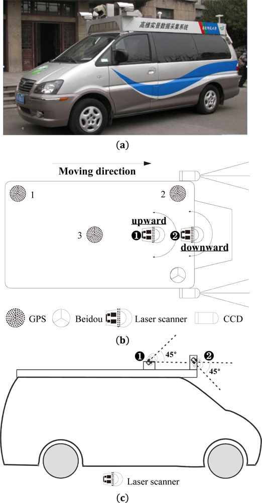
The Mobile Laser Scanning data used in this study were collected by the MLS System of East China Normal University (ECNU-MLS) (Figure 1(a)). It consists of a carrying platform (a van), two laser scanners, three GPS receivers, a Beidou Navigation Satellite System (the global satellite navigation system of China) receiver, two CCD cameras, and other instruments.
In ECNU-MLS, laser scanners, GPS receivers, Beidou receiver, and CCD cameras are fixed on the top of the van (Figure 1(b)). Number one and two GPS receivers are used to calculate the moving direction, while the number three GPS receiver is used for timing and determining geographical location (Figure 1(b)). The Beidou receiver is used for location determination and communication. In addition, the CCD Cameras are utilized to get time series stereo pair images.
As shown in Figure 1(c), the first laser scanner is looking upward up to 45° above the horizon and the second scanner is looking downward 45° below the horizon. Both scanners have a valid scanning range of 80 m and a 180° field of view. A scanning line is comprised of 181 sampling points. The scanning accuracy is ±15 mm.
The navigation and location of ECNU-MLS mainly rely on the GPS receivers. When the signal from Virtual Reference Station (VRS) is available for the GPS receivers, the location is determined by the Real Time Kinematic (RTK) technology with an absolute accuracy of 20 centimeters. When VRS signal is not available, the system provides the location with an accuracy of two meters. The Inertial Measurement Unit (IMU) installed in ECNU-MLS records the attitude data of the vehicle. The attitude data are used to correct the location information when VRS or GPS signals are not available.
The data collected by ECNU-MLS include 3D coordinates of scanning points, 3D coordinates of vehicle trajectory with a time interval of five seconds, and digital stereo image pairs. The 3D points, namely, laser scanning point cloud, contain geometric information about various urban street-scene objects, such as trees, buildings, street furniture, and other natural or man-made objects along roads. The MLS point cloud data collected by two laser scanners on the van and vehicle trajectory points are used in our study.
The original data are given in Geographical Coordinate System (longitude and latitude) with reference to the WGS 84 datum. In order to calculate length and area of objects, the longitude and latitude coordinates of original scanning points are projected to a planar x–y coordinate system of UTM (Zone 51N). The height (z) of the scanning points is referenced to the WGS 84 datum.
3. Methodology
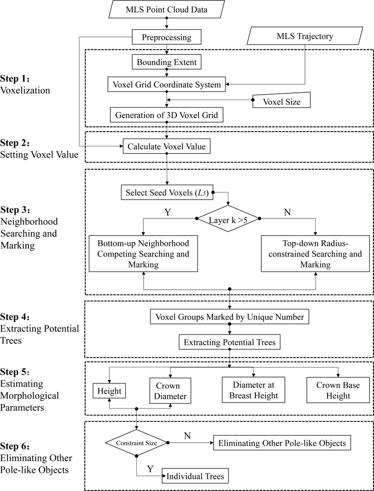
Our VMNS method contains 6 steps (Figure 2): (1) voxelization, (2) calculating values of voxels, (3) competing neighborhood searching and marking, (4) extracting potential trees, (5) deriving morphological parameters, and (6) elimination of pole-like objects other than trees.
3.1. Voxelization
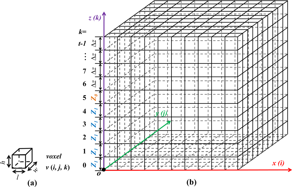
With the voxel data structure, the geographical space is conceptualized and represented as a set of volumetric elements (voxels) (Figure 3(b)). A voxel is a building block in the shape of a cuboid, and its geometry is defined by length (l), width (w), and height (h) (Figure 3(a)). The location of a voxel in 3D voxel grid system is indexed by column (i), row (j), and layer (k) (Figure 3(a,b)). Let v(i, j, k) denote a voxel, and v(*, *, k) denote the voxels in layer k (Lk). If the whole voxel grid system V has t voxel layers (Figure 3(b)), the voxel grid system can be defined as the union of all the layers (Equation (1)):
The first step of our VMNS method is voxelization (i.e., generating the voxel grid system) based on the dimensions of MLS point cloud. In order to illustrate the processing procedure of our method, we will first use the laser scanning point cloud and vehicle trajectory points collected in a relatively straight street segment with a flat surface and discuss the application of our method in more complicated situation afterwards. The coordinate system of the voxel grid system is set by the following rules:
The origin (O) of the voxel grid system is set to the point in which x–y coordinates (x0, y0) equal to the minimum x and y coordinate values of all laser scanning points, and its vertical coordinate equals to the height (zv) of the first point of vehicle trajectory.
The XY horizontal plane: X-axis is oriented in west-east direction, while Y-axis is oriented in south-north direction.
Z-axis is perpendicular to XY plane.
The length (l = Δx) and width (w = Δy) of all voxels in the voxel grid system are uniform, which can be specified by users. However, the height of the voxels may vary from the layer to layer. The voxel height for each layer is defined in Equation (2) (also see Figure 3(b)). The purpose of varying voxel height in different layers is to make sure the 6th voxel layer (L5) in the voxel grid corresponds to relative height of 1.2–1.4 m above the ground, which is usually used to measure the DBH of a tree in horticulture. The bounding extent of all laser scanning points is calculated. The range of the voxel grid system is set to be big enough to contain all laser scanning points.
3.2. Calculating Values of Voxels
After the voxelization, each laser scanning point will be associated with a voxel. If a laser scanning point has coordinate values (x, y, z), the column (i), row (j), and layer (k) of its corresponding voxel in the voxel grid is calculated in Equation (3).
It should be noted that the laser scanning data is collected on a relatively flat road, and the first trajectory point is regarded as the referenced ground level. The laser points below the ground are not considered in the neighborhood searching and marking.
After all laser scanning points have been associated with the corresponding voxels, a value is assigned to each voxel to indicate the number of laser scanning points falling into that voxel.
3.3. Searching and Marking Neighborhoods
3.3.1. Neighborhood of a Voxel
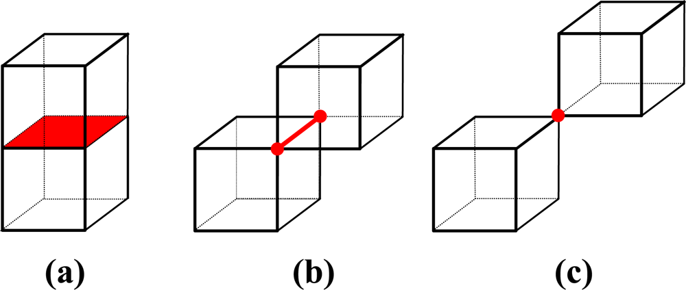
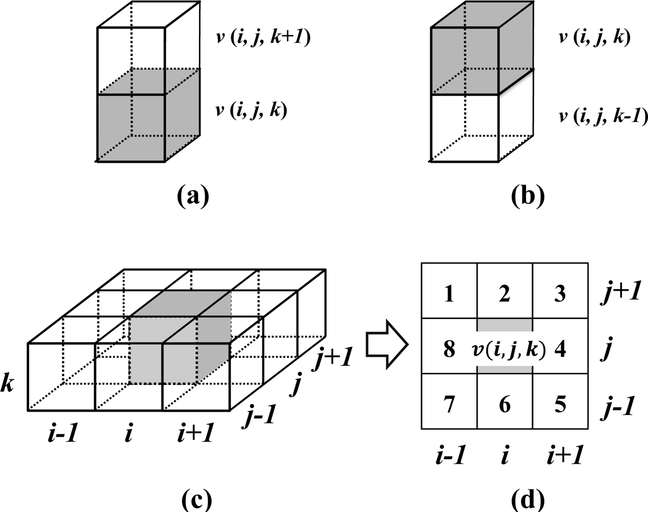
Neighborhood searching is an effective approach to dealing with the region growing problem in digital image processing. Our method extends traditional neighborhood searching from a 2D image plane to a 3D voxel grid system. In a voxel grid system, each voxel has three types of neighbors (Figure 4): face neighbors, edge neighbors, and vertex neighbors. In a vertical direction, a voxel v (i, j, k) has two types of face neighbor: top face neighbor (TFN) v (i, j, k+1) (Figure 5(a)) and bottom face neighbor (BFN) v (i, j, k−1) (Figure 5(b)). In the same layer, a voxel v (i, j, k) has 8-neighbors: 4 face neighbors (v (i+1, j, k), v (i−1, j, k), v (i, j+1, k), and v (i, j−1, k)) and 4 edge neighbors (v (i+1, j+1, k), v (i+1, j−1, k), v (i−1, j+1, k), and v (i−1, j−1, k)) (Figure 5(c)). As shown in Figure 5(d), if the voxel height is neglected, the voxels in the same layer can be treated as a regular pixel grid.
In our study, TFN, BFN, and 8-neighbors in the same layer of a voxel are used to define a 3D neighborhood in the voxel grid system for searching and marking. TFN and BFN represent the vertical connections of voxels. They can be used to detect the vertical stretches of a tree, namely the tree trunk. 8-neighbors in the same layer represents the connection of voxels in the XY-plane, which is used for detecting the horizontal cross-sections of three crowns.
3.3.2. Select Seed Voxels
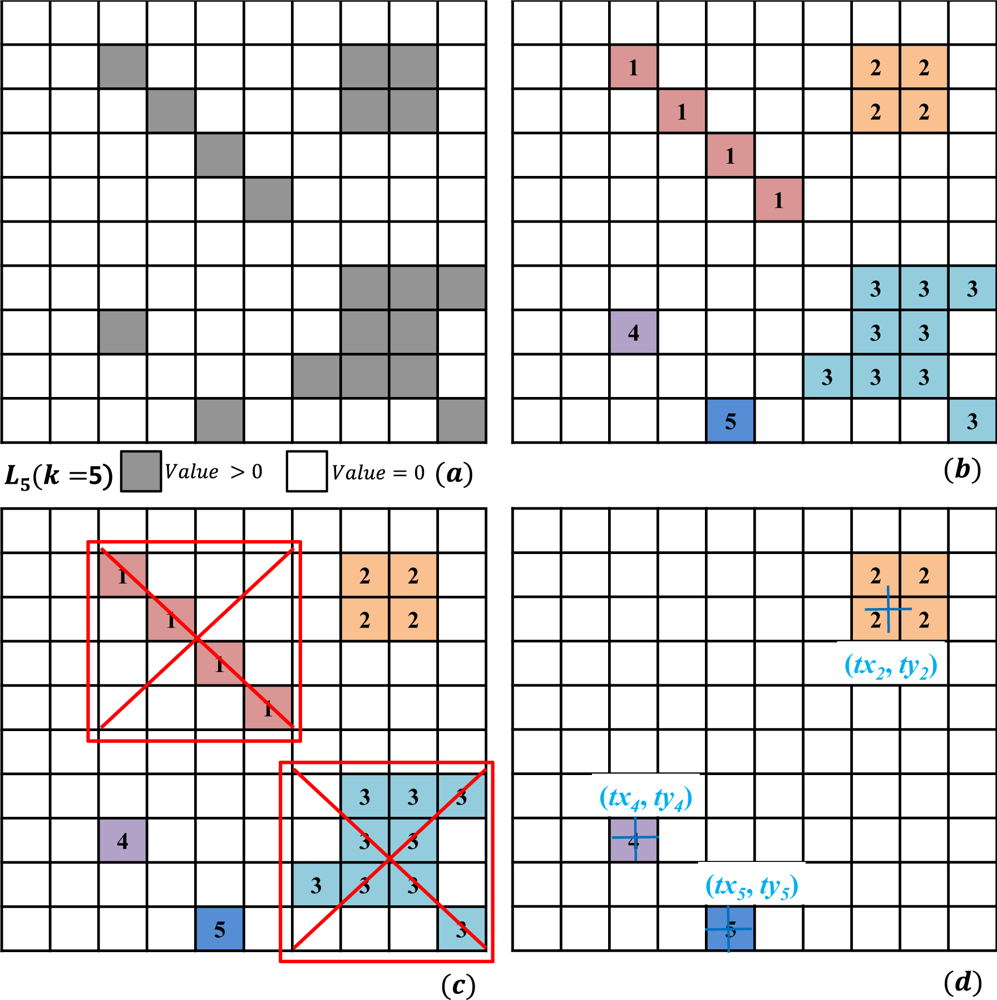
A set of hypothetical voxel layers are given in Figures 6(a), 7(a), 8(a), and 9(a) to illustrate the neighborhood searching and marking procedure. The voxels in grey represent those with a value larger than 0 (i.e., at least one laser scanning point is contained in the voxel). Such voxels, referred to as foreground voxels in this paper, represent a part of an object. The voxels in white represents the voxels with a value of 0. These white voxels are empty and no scanning laser points are detected and, hence, are treated as background voxels.
The searching for tree objects starts with the seed voxels. In order to eliminate the influence of the non-tree objects near the ground, we initiate searching at the voxel layer (L5) in the voxel grid system (Figure 6(a)). As explained in Section 3.1, L5 is located at a relative height of 1.2–1.4 m above the ground, which is usually used to measure the DBH of a tree in horticulture. We assume that a laser scanning point reflected by the tree trunk will be detected in layer L5 if a street tree is presence at that location.
All the voxels at the layer L5 are scanned in a row-wise manner. The first foreground voxel detected in the scanning is used as a seed voxel for region growing and marking. The seed voxel is expanded to include all foreground voxels that are located in the 8-neighbors of the seed voxel in the same layer. The expansion is continuing recursively until all connected voxels are included and grouped (Figure 6(b)). The voxels in a same group are indexed and marked incrementally with a unique integer number (g) (Figure 6(b)).
If a marked voxel group at layer L5 contains the laser scanning points reflected by the tree trunk, the detected voxel group should have two geometric properties: (1) the area of voxels projected to the horizontal plane should be relatively small, in comparison with buildings and other non-tree objects and (2) the shape of voxel group projected to the horizontal plane should be compact and approximately have a circular shape. To discriminate tree objects from other urban street objects, two morphological attributes for each voxel group are calculated, after all the foreground voxels in layer L5 are grouped. One is the number (n) of voxels in the group, which represents the area of voxels projected to the horizontal plane. The other is the compactness index (CI, defined in Equation (4)) of voxel group in the horizontal plane. If the shape of voxel group is in a perfect circle, its CI is 1.0. On the contrary, the shape is away from the circle, CI will have a smaller value than 1.0. In order to get reliable seed voxels of street trees, if n is larger than a threshold value (N0) or CI is less than a threshold value (CI0), the voxel group is not considered to belong to a tree and will be removed from further processing (Figure 6(c)).
After removal of the voxel groups that are assessed as non-tree objects, the remaining voxel groups are regarded as potential tree objects for further processing. All the potential trees have the same index numbers as the voxel groups (g). The location coordinates of a potential tree g trunk (txg, tyg) (Equation (7)) is calculated as the horizontal centroid of all laser scanning points contained by the voxel group (Figure 6(d)).
Then, a top-down radius-constrained searching and marking process is preformed to identify the lower part of tree trunk. It is immediately followed by a bottom-up neighborhood competing searching and marking process to identify upper part of tree trunk and tree crown.
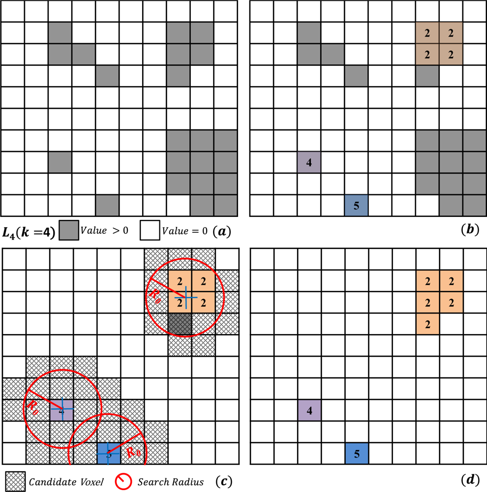
3.3.3. Top-Down Radius-Constrained Searching and Marking
The top-down radius-constrained searching and marking method is used to identify the voxels constituting the trunk part in the voxel layers below L5. Figure 7 illustrates the search and marking process in voxel layer L4. In the searching and marking process in layer Lk (0 ≤ k < 5), the foreground voxels (i.e., value > 0) in the bottom face neighbors of the seed voxels in layer Lk+1 will be marked with the same group number as the voxel group in layer Lk+1 first (Figure 7(b)). Those marked voxels in layer Lk are the seed voxels of neighborhood searching and marking in this layer.
In order to reduce the influence of other objects near the ground, the search is constrained to a circle with radius R0 (Figure 7(c)) around the location point of each potential tree trunk in the horizontal plane (see Figure 6(d)). For the voxel group g, the voxels within the search circle are the candidates for its own region growing and marking (Figure 7(c)). The candidate voxels located in the 8-neighbors of the seed voxels of group g in layer Lk are marked with the same group number g (Figure 7(d)).
The top-down searching and marking proceeds recursively until the 1st layer of the voxel grid system (L0) has been searched and marked.
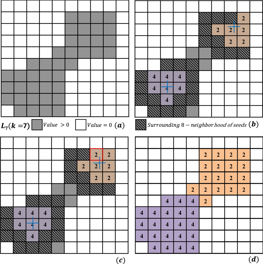
3.3.4. Bottom-Up Neighborhood Competing Searching and Marking
The bottom-up neighborhood competing searching and marking algorithm is used to identify the voxels constituting the upper trunk and crowns of street trees in the voxel layers above layer L5. Figures 8 and 9 illustrate the processes in voxel layers L6 and L7.
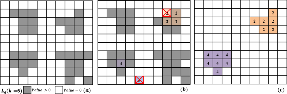
The bottom-up search starts in layer L6 (the 7th layer in the voxel grid, Figure 8(a)), and proceeds recursively to a higher layer (L7 (Figure 9(a)), L8, …, Lt−1). In the searching and marking process in layer Lk (k >5), if the top face neighbors of the seed voxels in layer Lk−1 are foreground voxels, they will be marked with the same group number as the voxel group in layer Lk−1 (Figures 8(b) and 9(b)). If not, they will be removed from the seed voxels and no longer be considered in subsequent processing (Figure 8(b)). Those marked voxels in Lk are the seed voxels of neighborhood searching and marking in this layer.
Ideally, if there is a gap between crowns of two street trees, (e.g., Figure 8(b)), the neighborhood expansion of foreground voxels from the seed voxels would result in two separate tree objects (Figure 8(c)). However, in reality, the crowns of two adjacent flourishing street trees often touch or overlap each other (e.g., Figure 9(a)). In this case, the conventional sequential neighborhood expanding and marking algorithm would mark all adjacent foreground voxels of two adjacent street trees into a single voxel group and consequently two tree objects cannot be correctly separated. To solve this difficult problem, we adapted a competing region growing algorithm [47] to separate the touching or interlocking tree crowns. In the traditional sequential region growing, all neighboring foreground voxels around seed voxels would be identified to form a marked voxel group, before starting the search and marking of next voxel group. In our competing region growing algorithm, the foreground voxel groups are incrementally expanded and grown, and which foreground voxel group is being grown in the next round expansion is governed by the competition rule.
As illustrated in Figure 9(b), for the seed voxels in layer Lk, their surrounding 8-neighbors voxels can be easily identified. For each voxel group, the distance from each surrounding 8-neighbors voxel to the center of corresponding tree trunk is calculated and sorted. The minimum distance (dg, g is the group number) for each foreground group is recorded. Among all of voxel groups, we select the voxel group whose minimum distance is the lowest to grow. The newly marked voxel (the voxel marked with a red box in Figure 9(c)) will be added to that group, and its 8-neighbors voxels will be checked. Next, the new dg value will be calculated and updated for this voxel group. Then, we enter into the next round of growing process by selecting the voxel group with the lowest dg value to grow. The above competing neighborhood searching and marking process is repeated, round by round, until all foreground voxels located in the 8-neighbors of seeds have been grouped and numbered (Figure 9(d)). The same bottom-up neighborhood competing searching and marking process will be sequentially applied to higher layers until the top layer of the voxel grid system is processed or the height of the layer is larger than a threshold value Hmax.
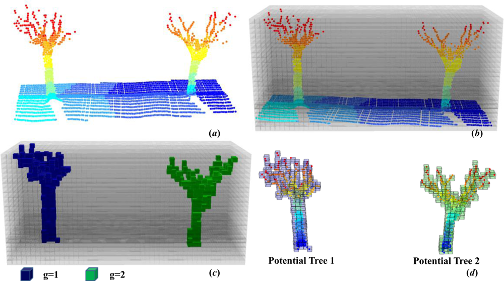
3.4. Extracting Potential Trees
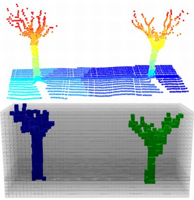
After the neighborhood searching and marking processes, the voxels in voxel grid system have been divided into two categories: marked voxel and non-marked voxel. The marked voxels with same group number are considered to contain the laser scanning points that constitute a potential individual street tree. For example, Figure 10(a) shows the original MLS point cloud in 3D view, and the height is coded in varying colors. After voxelization, a voxel grid is established (Figure 10(b)). Two groups have been marked in Figure 10(c) through the neighborhood searching and marking methods mentioned in section 3.3. Finally, the laser scanning points of two potential trees are identified and extracted (Figure 10(d)).
3.5. Estimating Morphological Parameters
Through the aforementioned process, each individual street tree is detected and represented by foreground voxels and associated laser scanning points. Four morphological parameters, including height, crown diameter, DBH, and CBH, are estimated for each tree based on the detected foreground voxels and associated laser scanning points inside these voxels.
3.5.1. Tree Height
A simple and straightforward algorithm to derive tree height (H) is to calculate the distance between the highest laser scanning point and the lowest one within the foreground voxel group constituting each tree object (Equation (8)):
3.5.2. Tree Crown Diameter
Conventionally, the crown diameter of a tree can be measured along two perpendicular directions from the location of the treetop [48]. In our study, we project all of the laser scanning points of the detected tree object to the horizontal plane. The range of the projected laser scanning points for each tree object in x and y directions are calculated. Namely, the differences between the maximum and minimum x and y coordinates of the projected points, denoted by CDx and CDy respectively, are calculated to indicate the tree crown diameter. We take the average value ( ) of CDx and CDy to approximate the tree crown diameter.
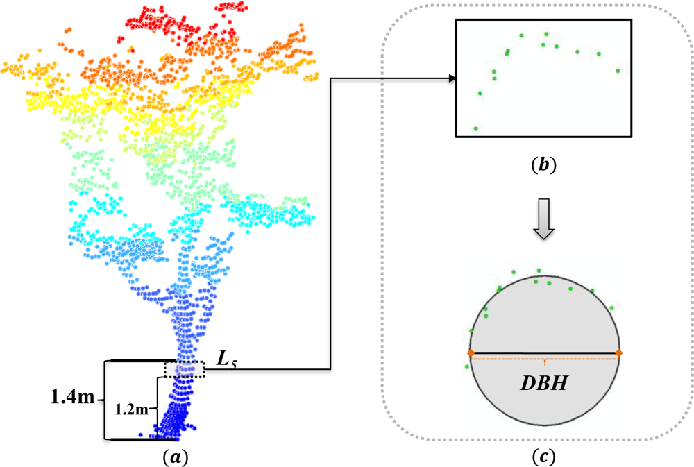
3.5.3. Diameter at Breast Height (DBH)
In the voxelization process, by adjusting height of different layers in the voxel grid system, we made the 6th voxel layer (L5) corresponds to the relative height of 1.2–1.4 m above the ground, which is usually used to measure the DBH of a tree in horticulture. After the laser scanning points of a tree are identified (Figure 11(a)) in the 6th voxel layer (L5), they are then projected to the horizontal plane (Figure 11(b)). Next, a circle is fitted to represent the horizontal cross-section shape of the trunk at breast height by using the least-squares best fitting technique (Figure 11(c)). The diameter of the fitted circle is taken as DBH.
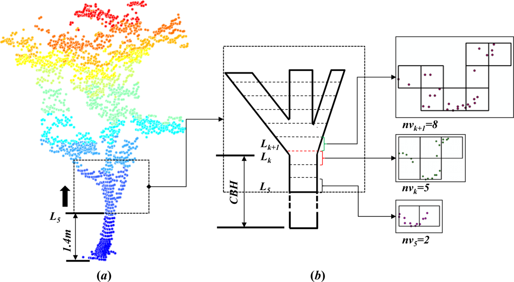
3.5.4. Tree Crown Base Height (CBH)
The crown base height is defined as the distance along the trunk from ground to the attachment point of the first living branch [49]. The critical issue in the crown base height estimation is to find the location of the attachment point of the first living branch. In the vertical profile of a tree, the living branch causes the sudden shape expansion in horizontal dimension. Since the detected tree object is represented as layers of voxels, a bottom-up layer by layer examination is able to locate the sudden shape expanding point.
The search for the sudden shape expansion point starts at the kth (k>5) voxel layer (Lk) in the grouped voxels of a tree (Figure 12(a)). The number of voxels (nvk) in Lk is calculated and recorded. The number of voxels in layer L5 is adopted as a reference number. During the bottom-up layer by layer examination, if the voxel number (nvk) at kth layer is larger than the threshold value (2·nv5) and the voxel number of its immediately higher layer (nvk+1) is also larger than the threshold value (2·nv5), then the kth layer is considered to contain the attachment point of the first living branch (Figure 12(b)). The CBH is calculated by differencing the average z value of the laser scanning points in layer Lk and the height of the lowest laser scanning point of that tree (Figure 12(b)).
3.6. Eliminating Pole-like Objects Other Than Trees
The selection of seed voxels may include pole-like objects other than trees, such as streetlights, electricity poles, concrete columns, etc. Therefore, the extracted grouped voxels may include some spurious non-tree pole like objects. We utilize a threshold value (CD0) of crown diameter and a threshold value (H0) of tree height to eliminate non-tree, pole-like objects. The extracted objects will be removed if H < H0 or CDx <CD0 OR CDy <CD0. The threshold values H0 and CD0 are adjustable according to the dominant species of street trees.
3.7. Software Tool Implementation
The VMNS method proposed in this paper has been implemented as a software tool to support the automated street tree extraction and parameters estimation by using ArcGIS Engine 10.0 and C# programming language in Microsoft Visual Studio 2010 environment. The required input data include the laser scanning points and vehicle trajectory points collected by ECNU-MLS. The software tool provides the graphical user interface for the users to specify and adjust the algorithm parameters and threshold values. The output results of the software tool include the extracted voxels constituting an individual street tree in Multipath format, the grouped laser scanning points for street trees, and a table of the estimated tree parameters.
4. Experimental Studies
Our VMNS algorithm and method was tested and evaluated through two case studies. The laser scanning point clouds for two case study areas were collected by using ECNU-MLS. To make the accuracy assessment of the derived tree parameters, we conducted the field survey of the street trees and the height and CBH of each street tree were measured by using a portable laser distance meter during field survey. The DBH of each tree was gauged by using metric fabric diameter tape. The crown diameters of each tree were measured with a tape in east-west and south-north directions (in the same directions as in the numerical algorithm).
4.1. Case Study 1
4.1.1. Data Collection and Voxelization
The first case study area (Figure 13(a)) is the East branch of Tongpu Road in the Putuo District of Shanghai. The mobile laser scanning point data were acquired on 14 March, 2012. The laser scanning point cloud consists of 866,222 sampling points covering a 332 m × 118 m street scene (Figure 13(a)) and the average point density is about 95 points/m2. The maximum height difference of the laser scanning points is 25.112 m. Street trees and other street objects, such as buildings, lights, and dustbins, are distributed along both sides of the road. The field measurements were taken on 15 March, 2012. Seventy-two street trees were visually identified about 6.5 m from the vehicle trajectory. The species of these trees are all Platanus acerifolia (Ait.) Willd. The average density of the laser scanning points of the street trees is about 212 points/m2. In this case study, Δx, Δy, and Δz of the voxel grid are 0.25 m, 0.25 m, and 0.25 m, respectively. A voxel grid system with 1,330 columns, 474 rows, and 101 layers is established. Among 63,672,420 voxels, 179,708 are identified as foreground voxels. The following threshold values are used for this case study: R0 = 0.5 m, N0 = 4, CI0 = 0.5, Hmax = 15 m, CD0 = 1 m, and H0 = 2 m.
4.1.2. Results
By using our VMNS method, 121 pole-like objects are detected as potential street trees, and 49 non-tree pole-like objects are eliminated based on the threshold values. As shown in Figure 13(b), all 72 street trees are identified correctly. Thus, the detection completeness and correctness are both 100% for this area. The location and 3D morphology of each tree are well represented by the laser scanning points.
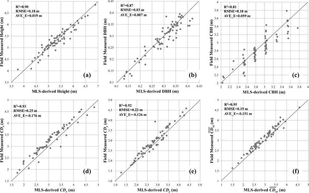
After street trees are identified, the laser scanning points and voxels that constitute an individual tree are used to calculate its morphological parameters, including height, DBH, crown diameter, and CBH. We compare the derived height, DBH, CBH, and crown diameter to the field measured values and calculate the average error (AVE_E) and root mean square error (RMSE) (Figure 14). Linear regression is also used to investigate the coefficient of determination relationships between the MLS-derived and field measured values of those parameters (Figure 14).
The results show that the estimated height and DBH based on our VMNS method have a relatively high accuracy. The R2 values of height and DBH are 0.90 and 0.87, respectively (see Figure 14(a,b)). The RMSE values for tree height and DBH are 0.18 m and 0.03 m. The R2 value for CBH is 0.81 (Figure 14(c)).
The crown diameter values of most street trees (71 trees) are between 1 m to 5 m. Only one tree has an extremely large crown diameter value of 10.70 m (average crown diameter in x and y direction). In order to avoid the extremely large value affect the correlation analysis, this tree is not included in correlation analysis in Figure 14(d–f). A good agreement between the numerically derived tree parameter values and the field-measured values are indicated by very high correlation coefficients and low RMSEs. The R2 of CDx, CDy, and are 0.93, 0.92, and 0.95 (Figure 14(d–f)), and corresponding RMSEs are 0.25 m, 0.22 m, and 0.19 m, respectively.
4.2. Case Study 2
4.2.1. Data Collection and Parameters Setting
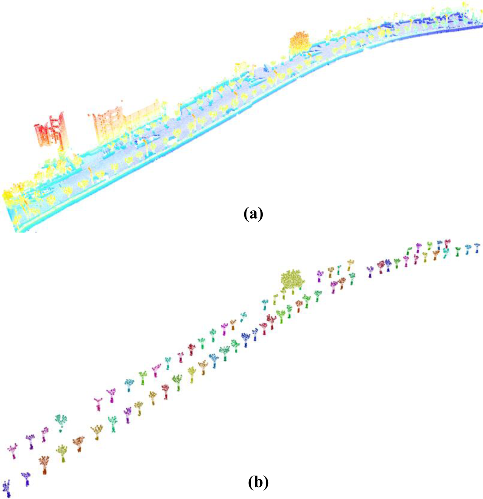
The second case study area (Figure 15(a)) is the West branch of Zixing Road in the Minhang District of Shanghai, and scanning point cloud data were collected on 7 December, 2012. The road section to be investigated is approximately transmeridional and has a length of 240 m. The laser scanning point cloud consists of 691,181 sampling points covering a 211 m × 117 m street segment, and the average point density is about 113 points/m2. The maximum height difference of the laser scanning points is 11.638 m. The field measurements of the trees were conducted on 18 December, 2012. Sixty-eight street trees were visually detected, which are about 5 m away from the vehicle trajectory. The species of all these trees is Cinnamomum camphora (L.) Presl. The average density of the laser scanning points over the street trees is about 224 points/m2. In this case study, Δx, Δy, and Δz of the voxel grid are set to 0.25 m, 0.25 m, and 0.25 m, respectively. A voxel grid system with 844 columns, 468 rows, and 47 layers is established. One hundred eighty-two thousand five hundred eighty-four voxels are identified as foreground voxels. The threshold values used in this case study are: R0 = 0.5 m, N0 = 4, CI0 = 0.5, Hmax = 10 m, CD0 = 1 m, and H0 = 2 m.
4.2.2. Results
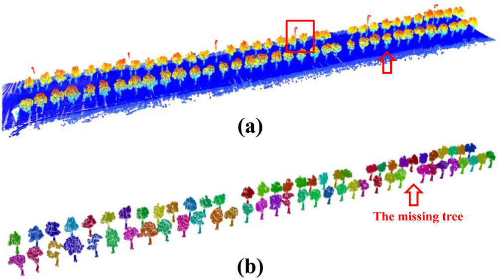
By using our VMNS method, 76 pole-like objects are detected as potential street trees. Nine of them were filtered out as non-tree objects based on the threshold values. As shown in Figure 15(b), 67 street trees are identified correctly, and only one tree was missed with our method. Thus, the detection completeness rate is 98.52% and correctness rate is 100% for this area.
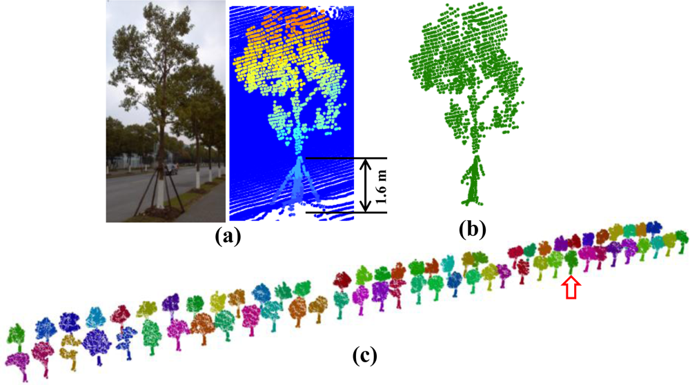
The reason why one tree was not detected is that the wooden support structure with a height of 1.6 m was attached to the trunk of that tree (Figure 16(a)). Since we selected the seed voxels in the 6th layer located at relative height of 1.2–1.4 m above the ground, the seeds voxels’ number for the missing tree was larger than the threshold and therefore was excluded for further processing. In order to solve this problem, we adjusted the height of the 6th layer to 1.8–2.0 m for all the street trees in case study 2, for the season that their CBHs are larger than two meters. After the fine-tuning of this algorithm parameter, the missing tree was identified and delineated with our method (Figure 16(b,c)). The location and 3D morphology of all 68 trees are shown in (Figure 16(c)).
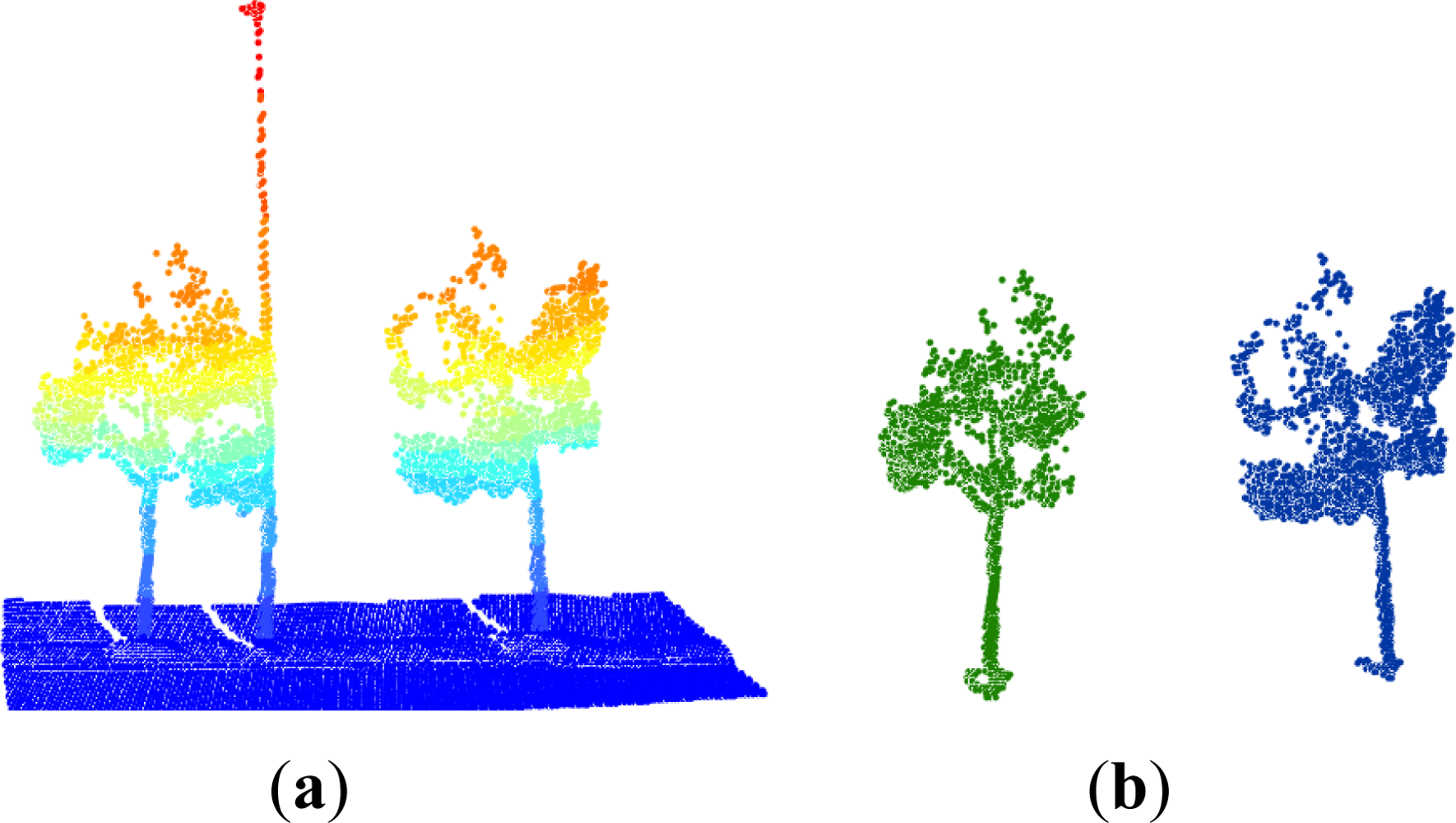
As indicated in Figure 15(a), the poles of some streetlights are attached to the neighboring trees. For example, a streetlight, marked by the red box in Figure 15(a), touched the adjacent tree crown (see Figure 17(a)). From the processing result shown in Figure 17(b), our method is robust enough to handle this complicated situation, and the trees were correctly extracted and streetlight poles successfully filtered out. The intelligence and capability of our method in handling this complex situation is due to the competing neighborhood searching algorithm and the use of the shape information of horizontal cross-sections of the tree at different height.
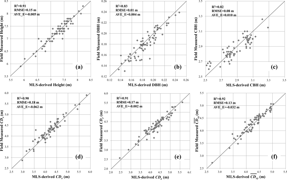
After street trees were detected and separated, the laser scanning points and voxels that form an individual tree are used to calculate its morphological parameters. The comparison between the derived three heights, DBH, CBH, and crown diameter and the field measurements is shown in Figure 18. The R2 values of height, DBH, and CBH are 0.91, 0.83, and 0.82 respectively (see Figure 18(a–c)). RMSE values for these parameters are 0.15 m, 0.01 m, and 0.08 m, respectively. The crown diameter values of all 68 trees range from 2.7 m to 5 m. The R2 for CDx, CDy, and are 0.90, 0.91, and 0.92 (Figure 18(d–f)), and RMSEs are 0.18 m, 0.17 m, and 0.13 m, respectively.
4.3. Discussions
4.3.1. Tuning of the Algorithm Parameters
Two case study areas are located in different districts of Shanghai. Street trees and other street objects, such as buildings, lights, traffic signs, and dustbins, are presented along two sides of the roads. In Shanghai and other Chinese cities, trees of the same species are frequently planted along a road for the sake of easy horticultural management and aesthetic consideration. Because the trees along a specific segment of a road were often planted or transplanted in the same period and grew under similar conditions, as a result the size and shape of most trees for a certain road segment are quite similar. Thus, the case study areas used in our analysis represent the typical street scene in the urban area of Shanghai. For urban street trees with more complex structures, some pre-processing steps for original laser scanning point cloud, such as partitioning of data along road direction [44], removing the points that are far away from the survey trajectory, would simplify and improve the detection and quantification of street trees.
In the voxelization, the vertical origin of voxel grid system is set to the same elevation as the first point of vehicle trajectory. In our case studies, we assume that the ground surface of the road segment under processing has a constant elevation since the laser scanning data used in our case studies were collected over relatively straight streets with quite flat surfaces. Their maximum elevation differences are within one meter. For more complicated urban environments with curved streets, or streets with varying slopes, some data processing steps should be performed before applying our algorithm and method. In these more complicated situations, one data processing strategy is to partition the road into several smaller segments. For each small road segment, the street trees would be more homogeneous, and a set of appropriate algorithm parameters can be selected for our method to get accurate detection results. Sequential processing of the laser scanning point cloud data from segment to segment along the road would improve the detection accuracy and reliability. The other preprocessing strategy is to model the vehicle trajectory using a polynomial mathematical function, and then normalize the heights of laser scanning point cloud data to the values relative to the road surface represented by the polynomial function. When some irregular structures, or other objects, are present near street trees (e.g., Figure 16(a)), the use of default algorithm parameters may fail the seed voxels searching and cause the omission error in tree detection. As demonstrated in the second case study, the algorithm parameters and threshold values used in our method are adjustable. By fine-tuning the algorithm parameters and threshold values according to the urban street situation, the omission error can be fixed.
4.3.2. Accuracy Comparison
The two case studies show that the tree heights derived from our VMNS method have a relatively high accuracy. In comparison with field measurements, the R2 values for the two study areas are larger than 0.9. For DBH, its R2 value is slightly lower than for tree height, but the RMSEs for DBH are as low as 0.03 m in the first case study area, and 0.01 m in the second case study area, which are comparable to other studies (e.g., 0.021 m reported by [35]). The R2 values for CBH in the two case studies are 0.81 and 0.82, which are better than the results reported by using ALS data (e.g., 0.49 to 0.80 reported in [46]). The RMSEs for CBH are less than 0.1 m, which are much smaller than the values (about 2 m) reported in [46].
For the crown diameter estimation, the R2 values for CDs (x direction, y direction, and average) are larger than 0.9 in the two case studies, which are much better than the results reported by using ALS data, i.e., 0.44 reported in [50] and 0.63 reported in [48]. It should be noted that previous studies on the crown diameter estimation by using ALS data mostly focus on natural forest regions. As the density of trees cluster is high and many tree crowns are interlocked, segmenting individual trees in natural forest areas from ALS data is more difficult in comparison with separating urban street trees with MLS data. Consequently, the crown diameter estimation with MLS data is easier and more reliable in comparison with processing ALS data.
Figures 14(b) and 18(b) indicate that the average error of DBH estimations for the two case studies are 0.007 and 0.004. Our method overestimated the tree diameter in comparison with field measurements. This is primarily due to the limitation of laser scanning density and the side looking geometry of the MLS system. As indicated in Figure 11(c), only a few laser points reflected from the front side of tree trunk facing the road were captured by the laser scanning system. Inadequate number of laser scanning points, particularly lack of laser scanning sampling points from back side of tree trunks adversely affect the circle fitting and hence the tree diameter estimation accuracy. Our method underestimated crown diameters (Figure 14(d–f), and Figure 18(d–f)), particularly in the first case study. The species of street trees in the first case study area is Platanus acerifolia (Ait.) Willd, a typical deciduous tree. When the laser scanning data was collected in March, the trees were still in leave-off status. The edge of tree crowns, without flourishing leaves, cannot be fully depicted by the limited density of laser scanning point cloud.
5. Conclusions
This paper presents a novel Voxel-based Marked Neighborhood Searching (VMNS) method for automated identification and morphological parameters estimation for individual street trees based on Mobile Laser Scanning (MLS) point cloud data. Our VMNS method is comprised of six technical steps: voxelization, calculating voxel values, neighborhood searching and marking, extracting potential trees, estimating morphological parameters, and eliminating non-tree pole-like objects. In contrast to the use of a uniform constant voxel height in the voxelization process in many other studies, our method adopted variable voxel height for different voxel layers in order to improve the flexibility and accuracy for street tree extraction and tree morphological parameter estimations. We extended the traditional neighborhood searching from a 2D image grid to a 3D voxel grid system in our method. A top-down radius-constrained searching and marking, immediately followed by a bottom-up competing neighborhood searching and marking processes are designed to identify and group the foreground voxels belonging to a potential individual street tree. The consecutive processing of the MLS point cloud through the six technical steps, our method is capable of generating a voxel-based 3D model for each individual street tree and identifying associated laser scanning points belonging to each individual tree. The tree morphological parameters, including tree height, crown diameter, diameter at breast height (DBH), and crown base height (CBH), of individual street tree have been calculated with satisfactory accuracy.
The primary innovations of our method are threefold. First, the consecutive neighborhood searching and marking algorithms make full use of spatial proximities both in vertical and horizontal directions of laser scanning points, constituting an individual tree into account by adopting an adjustable voxelization scheme. This enables us to construct a voxel-based morphological model for each tree. This represents a major technical improvement over 2D neighborhood search methods in the literature. Second, we embedded a competing neighborhood searching and growing algorithm in the bottom-up search and marking process. This algorithm component represents a critical technical innovation. As demonstrated, this technical innovation enables the separation of touching and overlapping tree crowns and, therefore, make our method more robust and reliable than in previous studies. Third, our study represents the first research effort in the automated derivations of a set of morphological parameters of street trees based on MLS data.
Two case studies demonstrate that our VMNS method is effective and efficient to form 3D voxel models and derive morphological parameters for individual street trees. The detection completeness and correctness rates are over 98% for the case study areas. The estimated morphological parameters have been compared to in situ field measurements. The comparisons show tree height, crown diameter, DBH, and CBH, estimated from our method are in a good agreement with field measurements, and the RMSEs are small. In two case studies, the R2 values for tree height and crown diameter are over 0.9, and for DBH and CBH are over 0.8. Our results are more accurate and reliable, in comparison with previous studies reported in literature.
There are still some limitations to our method. Our method is difficult to extract the multiple-stemmed street trees if their furcal sections are lower than the initial searching height. The multiple stems of an individual tree would be detected as several separated trees. The method is tested only through two case study areas in Shanghai. In the future research, we will test and improve the method through other study areas and make further improvements on the algorithms for estimating morphological parameters of individual trees. In addition, we will include other important morphological parameters, such as crown project area, green volume, and leaf area index of street trees.
Acknowledgments
This study is supported by the National Natural Science Foundation of China (No. 41001270 and No. 41071275), the Specialized Research Fund for the Doctoral Program of Higher Education (No. 20100076120017), and the Fundamental Research Funds for the Central Universities of China. The authors thank four anonymous reviewers for their constructive comments and suggestions. In addition, we also thank Haitao Yan, Rui Liu, Linhua Xiong, and Siyi Yu from East China Normal University for helping us to collect the field data.
References
- Stovin, V.R.; Jorgensen, A.; Clayden, A. Street trees and stormwater management. Arboricul. J 2008, 30, 297–310. [Google Scholar]
- Ries, K.; Eichhorn, J. Simulation of effects of vegetation on the dispersion of pollutants in street canyons. Meteorologische Zeitschrift 2001, 10, 229–233. [Google Scholar]
- Tallis, M.; Taylor, G.; Sinnett, D.; Freer-Smith, P. Estimating the removal of atmospheric particulate pollution by the urban tree canopy of London, under current and future environments. Landsc. Urban Plan 2011, 103, 129–138. [Google Scholar]
- Gromke, C.; Buccolieri, R.; Di Sabatino, S.; Ruck, B. Dispersion study in a street canyon with tree planting by means of wind tunnel and numerical investigations—Evaluation of CFD data with experimental data. Atmos. Environ 2008, 42, 8640–8650. [Google Scholar]
- Fang, C.F.; Ling, D.L. Investigation of the noise reduction provided by tree belts. Landsc. Urban Plan 2003, 63, 187–195. [Google Scholar]
- Ali-Toudert, F.; Mayer, H. Effects of asymmetry, galleries, overhanging facades and vegetation on thermal comfort in urban street canyons. Sol. Energy 2007, 81, 742–754. [Google Scholar]
- Mackey, C.W.; Lee, X.; Smith, R.B. Remotely sensing the cooling effects of city scale efforts to reduce urban heat island. Build. Environ 2012, 49, 348–358. [Google Scholar]
- Shashua-Bar, L.; Hoffman, M.E. Vegetation as a climatic component in the design of an urban street—An empirical model for predicting the cooling effect of urban green areas with trees. Energy Build 2000, 31, 221–235. [Google Scholar]
- Akbari, H. Shade trees reduce building energy use and CO2 emissions from power plants. Environ. Pollut 2002, 116, S119–S126. [Google Scholar]
- Jutras, P.; Prasher, S.O.; Mehuys, G.R. Prediction of street tree morphological parameters using artificial neural networks. Comput. Electron. Agric 2009, 67, 9–17. [Google Scholar]
- Gilbertson, P.; Bradshaw, A.D. The survival of newly planted trees in inner cities. Arboricul. J 1990, 14, 287–309. [Google Scholar]
- Nowak, D.J.; McBride, J.R.; Beatty, R.A. Newly planted street tree growth and mortality. J. Arboricul 1990, 16, 124–129. [Google Scholar]
- Gong, P.; Li, Z.; Huang, H.B.; Sun, G.Q.; Wang, L. ICESat GLAS Data for urban environment monitoring. IEEE Trans. Geosci. Remote Sens 2011, 49, 1158–1172. [Google Scholar]
- Lefsky, M.; McHale, M. Volume estimates of trees with complex architecture from terrestrial laser scanning. J. Appl. Remote Sens. 2008. [Google Scholar] [CrossRef]
- Van der Zande, D.; Hoet, W.; Jonckheere, L.; van Aardt, J.; Coppin, P. Influence of measurement set-up of ground-based LiDAR for derivation of tree structure. Agr. Forest Meteorol 2006, 141, 147–160. [Google Scholar]
- Van der Zande, D.; Jonckheere, I.; Stuckens, J.; Verstraeten, W.W.; Coppin, P. Sampling design of ground-based lidar measurements of forest canopy structure and its effect on shadowing. Can. J. Remote Sens 2008, 34, 526–538. [Google Scholar]
- Yu, B.; Liu, H.; Wu, J.; Lin, W.-M. Investigating impacts of urban morphology on spatio-temporal variations of solar radiation with airborne LIDAR data and a solar flux model: A case study of downtown Houston. Int. J. Remote Sens 2009, 30, 4359–4385. [Google Scholar]
- Haala, N.; Brenner, C. Extraction of buildings and trees in urban environments. ISPRS J. Photogram 1999, 54, 130–137. [Google Scholar]
- Yu, B.; Liu, H.; Wu, J.; Hu, Y.; Zhang, L. Automated derivation of urban building density information using airborne LiDAR data and object-based method. Landsc. Urban Plan 2010, 98, 210–219. [Google Scholar]
- Ma, R.J. DEM generation and building detection from Lidar data. Photogramm. Eng. Remote Sensing 2005, 71, 847–854. [Google Scholar]
- Huang, Y.; Yu, B.; Hu, Z.; Wu, J.; Wu, B. Locating Suitable Roofs for Utilization of Solar Energy in Downtown Area Using Airborne LiDAR Data and Object-Based Method: A Case Study of the Lujiazui Region, Shanghai. Proceedings of 2012 Second International Workshop on Earth Observation and Remote Sensing Applications (EORSA), Shanghai, China, 8–11 June 2012; pp. 322–326.
- Hecht, R.; Meinel, G.; Buchroithner, M.F. Estimation of urban green volume based on single-pulse LiDAR data. IEEE Trans. Geosci. Remote Sens 2008, 46, 3832–3840. [Google Scholar]
- Huang, Y.; Yu, B.; Zhou, J.; Hu, C.; Tan, W.; Hu, Z.; Wu, J. Toward automatic estimation of urban green volume using airborne LiDAR data and high resolution Remote Sensing images. Front. Earth Sci. 2012. Online First. [Google Scholar] [CrossRef]
- Secord, J.; Zakhor, A. Tree detection in urban regions using aerial lidar and image data. IEEE Geosci. Remote Sens. Lett 2007, 4, 196–200. [Google Scholar]
- Kim, S.; Hinckley, T.; Briggs, D. Classifying individual tree genera using stepwise cluster analysis based on height and intensity metrics derived from airborne laser scanner data. Remote Sens. Environ 2011, 115, 3329–3342. [Google Scholar]
- Wang, L.; Birt, A.; Lafon, C.; Cairns, D.; Coulson, R.; Tchakerian, M.; Xi, W.; Popescu, S.; Guldin, J. Computer-based synthetic data to assess the tree delineation algorithm from airborne LiDAR survey. Geoinformatica 2011, 17, 35–61. [Google Scholar]
- Zhao, H.J.; Shibasaki, R. A vehicle-borne urban 3-D acquisition system using single-row laser range scanners. IEEE Trans. Syst. Man Cybern. B 2003, 33, 658–666. [Google Scholar]
- Lehtomäki, M.; Jaakkola, A.; Hyyppä, J.; Kukko, A.; Kaartinen, H. Detection of vertical pole-like objects in a road environment using vehicle-based laser scanning data. Remote Sens 2010, 2, 641–664. [Google Scholar]
- Yang, B.; Wei, Z.; Li, Q.; Li, J. Automated extraction of street-scene objects from mobile lidar point clouds. Int. J. Remote Sens 2012, 33, 5839–5861. [Google Scholar]
- Graham, L. Mobile mapping systems overview. Photogramm. Eng. Remote Sensing 2010, 76, 222–228. [Google Scholar]
- Jaakkola, A.; Hyyppa, J.; Hyyppa, H.; Kukko, A. Retrieval algorithms for road surface modelling using laser-based mobile mapping. Sensors 2008, 8, 5238–5249. [Google Scholar]
- Manandhar, D.; Shibasaki, R. Vehicle-Borne Laser Mapping System (VLMS) for 3-D GIS. Proceedings of 2001 International Geoscience and Remote Sensing Symposium (IGARSS 2001), Sydney, NSW, Australia, 9–3 July 2001; pp. 2073–2075.
- Li, B.; Li, Q.; Shi, W.; Wu, F. Feature extraction and modeling of urban building from vehicle-borne laser scanning data. Int. Arch. Photogramm. Remote Sens. Spat. Inf. Sci 2004, 35, 934–939. [Google Scholar]
- Zhu, L.; Hyyppä, J.; Kukko, A.; Kaartinen, H.; Chen, R. Photorealistic building reconstruction from mobile laser scanning data. Remote Sens 2011, 3, 1406–1426. [Google Scholar]
- Jaakkola, A.; Hyyppa, J.; Kukko, A.; Yu, X.W.; Kaartinen, H.; Lehtomaki, M.; Lin, Y. A low-cost multi-sensoral mobile mapping system and its feasibility for tree measurements. ISPRS J. Photogram 2010, 65, 514–522. [Google Scholar]
- Hu, Y.; Li, X.; Xie, J.; Guo, L. A Novel Approach to Extracting Street Lamps from Vehicle-Borne Laser Data. Proceedings of 2011 19th International Conference on Geoinformatics (Geoinformatics 2011), Shanghai, China, 24–26 June 2011.
- Lin, Y.; Jaakkola, A.; Hyyppä, J.; Kaartinen, H. From TLS to VLS: Biomass estimation at individual tree level. Remote Sens 2010, 2, 1864–1879. [Google Scholar]
- Alexander, C. Delineating tree crowns from airborne laser scanning point cloud data using Delaunay triangulation. Int. J. Remote Sens 2009, 30, 3843–3848. [Google Scholar]
- Wang, M.; Tseng, Y.-H. Incremental segmentation of lidar point clouds with an octree-structured voxel space. Photogramm. Rec 2011, 26, 32–57. [Google Scholar]
- Yu, X.W.; Hyyppa, J.; Vastaranta, M.; Holopainen, M.; Viitala, R. Predicting individual tree attributes from airborne laser point clouds based on the random forests technique. ISPRS J. Photogram 2011, 66, 28–37. [Google Scholar]
- Edson, C.; Wing, M.G. Airborne Light Detection and Ranging (LiDAR) for individual tree stem location, height, and biomass measurements. Remote Sens 2011, 3, 2494–2528. [Google Scholar]
- Shen, Y.; Sheng, Y.; Zhang, K.; Tang, Z.; Yan, S. Feature extraction from vehicle-borne laser scanning data. Proc. SPIE 2008. [Google Scholar] [CrossRef]
- Rutzinger, M.; Pratihast, A.K.; Elberink, S.J.O.; Vosselman, G. Tree modelling from mobile laser scanning data-sets. Photogramm. Rec 2011, 26, 361–372. [Google Scholar]
- Pu, S.; Rutzinger, M.; Vosselman, G.; Oude Elberink, S. Recognizing basic structures from mobile laser scanning data for road inventory studies. ISPRS J. Photogram 2011, 66, S28–S39. [Google Scholar]
- Pollard, T.B.; Eden, I.; Mundy, J.L.; Cooper, D.B. A volumetric approach to change detection in satellite images. Photogramm. Eng. Remote Sensing 2010, 76, 817–831. [Google Scholar]
- Popescu, S.C.; Zhao, K. A voxel-based lidar method for estimating crown base height for deciduous and pine trees. Remote Sens. Environ 2008, 112, 767–781. [Google Scholar]
- Liu, H.X.; Wang, L.; Jezek, K.C. Automated delineation of dry and melt snow zones in antarctica using active and passive microwave observations from space. IEEE Trans. Geosci. Remote Sens 2006, 44, 2152–2163. [Google Scholar]
- Popescu, S.C.; Wynne, R.H.; Nelson, R.F. Measuring individual tree crown diameter with lidar and assessing its influence on estimating forest volume and biomass. Can. J. Remote Sens 2003, 29, 564–577. [Google Scholar]
- Holmgren, J.; Persson, A. Identifying species of individual trees using airborne laser scanner. Remote Sens. Environ 2004, 90, 415–423. [Google Scholar]
- Lee, H.; Slatton, K.C.; Roth, B.E.; Cropper, W.P. Adaptive clustering of airborne LiDAR data to segment individual tree crowns in managed pine forests. Int. J. Remote Sens 2010, 31, 117–139. [Google Scholar]


Share and Cite
Wu, B.; Yu, B.; Yue, W.; Shu, S.; Tan, W.; Hu, C.; Huang, Y.; Wu, J.; Liu, H. A Voxel-Based Method for Automated Identification and Morphological Parameters Estimation of Individual Street Trees from Mobile Laser Scanning Data. Remote Sens. 2013, 5, 584-611. https://doi.org/10.3390/rs5020584
Wu B, Yu B, Yue W, Shu S, Tan W, Hu C, Huang Y, Wu J, Liu H. A Voxel-Based Method for Automated Identification and Morphological Parameters Estimation of Individual Street Trees from Mobile Laser Scanning Data. Remote Sensing. 2013; 5(2):584-611. https://doi.org/10.3390/rs5020584
Chicago/Turabian StyleWu, Bin, Bailang Yu, Wenhui Yue, Song Shu, Wenqi Tan, Chunling Hu, Yan Huang, Jianping Wu, and Hongxing Liu. 2013. "A Voxel-Based Method for Automated Identification and Morphological Parameters Estimation of Individual Street Trees from Mobile Laser Scanning Data" Remote Sensing 5, no. 2: 584-611. https://doi.org/10.3390/rs5020584